DART-Ray: a 3D ray-tracing radiative transfer code for calculating the propagation of light in dusty galaxies
Abstract
We present DART-Ray, a new ray-tracing 3D dust radiative transfer (RT) code designed specifically to calculate radiation field energy density (RFED) distributions within dusty galaxy models with arbitrary geometries. In this paper we introduce the basic algorithm implemented in DART-Ray which is based on a pre-calculation of a lower limit for the RFED distribution. This pre-calculation allows us to estimate the extent of regions around the radiation sources within which these sources contribute significantly to the RFED. In this way, ray-tracing calculations can be restricted to take place only within these regions, thus substantially reducing the computational time compared to a complete ray-tracing RT calculation. Anisotropic scattering is included in the code and handled in a similar fashion. Furthermore, the code utilizes a Cartesian adaptive spatial grid and an iterative method has been implemented to optimize the angular densities of the rays originated from each emitting cell. In order to verify the accuracy of the RT calculations performed by DART-Ray, we present results of comparisons with solutions obtained using the DUSTY 1D RT code for a dust shell illuminated by a central point source and existing 2D RT calculations of disc galaxies with diffusely distributed stellar emission and dust opacity. Finally, we show the application of the code on a spiral galaxy model with logarithmic spiral arms in order to measure the effect of the spiral pattern on the attenuation and RFED.
1 Introduction
Interstellar dust is of primary importance in determining the spectral energy distribution (SED) of the radiation
escaping from galaxies at wavelengths ranging from the ultraviolet (UV) to the submillimetre (submm) and radio. Dust attenuates and
redistributes the light,
originating
mainly from stars and, if present, from an active galactic nucleus (AGN), by either absorbing or scattering photons. The absorbed luminosity is then re-emitted
in the infrared regime. The dust may be situated in complex geometries with respect to these sources, affecting the observed structure
of the galaxy at each wavelength as well as its integrated SED.
Modeling the propagation of light within real galaxies is thus a challenging task. Nevertheless, it is essential to do such modeling,
if physical quantities of interest,
such as the distribution and properties of the stellar populations and the interstellar medium (ISM) as traced by dust and the interstellar radiation fields,
are to be derived from multiwavelength images and SEDs.
Taking advantage of the approximate cylindrical symmetry of galaxies, 2D dust radiative transfer (RT) models, such as the one presented by
Popescu et al. (2011), already contain the main ingredients needed to predict integrated galaxy SEDs, average profiles, dust emission and
attenuation for the case of normal star-forming disc galaxies. However, there are a number of reasons why 3D dust RT codes are desirable. First, spiral
galaxies, although well modeled with 2D codes, show the presence of multiple and irregular features such as spiral structures, bars,
warps and local clumpiness of the ISM. Also, galaxies may host a central AGN whose polar axis may not be aligned with that of the galaxy.
For mergers or post-merger galaxies there is clearly no fundamental symmetry of the distribution of stars and dust.
Finally, solutions for the distribution of stars and ISM provided by numerical simulations of forming and evolving galaxies
generally require processing with a 3D RT code in order to predict the appearance in different bands.
The main challenge in realizing 3D solutions of the dust RT problem is the computational expense. The
stationary 3D dust RT equation is a non-local non-linear equation: non-local in space (photons propagate within the entire
domain), direction (due to scattering, absorption/re-emission) and wavelength (absorption/re-emission). Even using a relatively coarse
resolution in each of the six fundamental variables, namely the three spatial coordinates, the two angles specifying the radiation
direction and the wavelength, solving the 3D dust RT
problem require an impressive amount of both memory and computational speed, at the limits of the capabilities of current computers.
Possibly the quickest way to calculate an image of a galaxy in direct and scattered light in a particular direction is by using Monte Carlo (MC) methods (including modern acceleration techniques, see Steinacker et al. 2013). There is a rich history of applications of MC codes to dust RT problems, starting with the pioneering works of e.g. Mattila (1970), Roark, Roark & Collins (1974), Witt & Stephens (1974) and Witt (1977). In the following decades the MC RT technique was further developed by many authors such as e.g. Witt, Thronson & Capuano (1992), Fischer, Henning & Yorke (1994), Bianchi, Ferrara & Giovanardi (1996), Witt & Gordon (1996) and Dullemond & Turolla (2000). Nowadays, this method can be considered as the mainstream approach to 3D dust RT calculations (see e.g. Gordon et al. 2001, Ercolano et al. 2005, Jonsson 2006, Bianchi 2008, Chakrabarti & Whitney 2009, Baes et al. 2011, Robitaille 2011, but also see table 1 of Steinacker et al. 2013 for a recent list of published 3D dust RT codes). The MC approach to dust RT consists of a simulation of the propagation of photons within a discretized spatial domain, based on a probabilistic determination of the location of emission of the photons, their initial propagation direction, the position where an interaction event (absorption or scattering) occurs and the new propagation direction after a scattering event. Thus, the MC technique mimics closely the actual processes occurring in nature which shape the appearance of galaxies in UV/optical light. However, since it is based on a probabilistic approach to determine the photon propagation directions, an RT MC calculation does not necessarily determine the radiation field energy density (RFED) accurately in the entire volume of the calculation. The reason is that regions which have a low probability of being illuminated are reached by only few photons unless the total number of photons in the RT run is substantially increased. Nonetheless, in the case of disc galaxies, accurate calculation of radiation field intensities throughout the entire volume is needed, in particular for the calculation of dust emission. Indeed, far-infrared/submm observations of spiral galaxies show that most of the dust emission luminosity is emitted longwards of 100m (see e.g. Sodroski et al. 1997, Odenwald et al. 1998, Popescu et al. 2002, Popescu & Tuffs 2002, Dale et al. 2007, 2012, Bendo et al. 2012) through grains situated in the diffuse ISM which are generally located at very considerable distances from the stars heating the dust.
Another method to solve the RT problem in galaxies, alternative to the mainstream MC approach, is by using a ray-tracing
algorithm. This method consists in the calculation of
the variation of the radiation specific intensity along a finite set of directions, usually referred to as ”rays”. Ray-tracing algorithms
can be specifically designed to calculate radiation field intensities throughout the entire volume considered in
the RT calculation. Also, it should be pointed out that MC codes already make large use of ray-tracing operations (see Steinacker et al.
2013). It is thus interesting to pursue
in the developing of pure ray-tracing 3D RT codes, which can be sufficiently efficient for the modelling of galaxies with
3D arbitrary geometries, if appropriate acceleration techniques are implemented. Similar to MC codes, ray-tracing dust RT codes have
had a rich history in astrophysics (see e.g. Hummer & Rybicki 1971, Rowan-Robinson
1980, Efstathiou & Rowan-Robinson 1990, Siebenmorgen et al. 1992,
Semionov & Vansevic̆ius 2005, 2006). Application to analysis of
galaxies started with the 2D code of Kylafis & Bahcall (1987). Although originally implemented only for the calculation of optical
images (see also Xilouris et al. 1997, 1998,1999), this algorithm was later adapted by Popescu et al. (2000) for the
calculation of radiation fields and was coupled with a dust emission model (including stochastic heating of grains) to predict the full
mid-infrared (MIR)/FIR/submm SED of spiral galaxies (see also Misiriotis et al. 2001, Popescu et al. 2011). Thus far, extensions of the ray-tracing
technique to 3D have been implemented but are specifically designed
for solving the RT problem for star forming clouds (e.g. Steinacker et al. 2003, Kuiper et al. 2010), heated by few dominant
discrete sources, rather than for very extended distributions of emission and dust as encountered in galaxies.
In this paper, we present DART-Ray11
1
The name of the code can be seen as the acronym for “Dust Adaptive Radiative Transfer Ray-tracing”
, a new ray-tracing
algorithm which is optimized for the solution of the 3D dust RT problem for
galaxies with arbitrary geometries and moderate optical depth at optical/UV wavelengths22
2
The actual version of the code
does not consider the dust
absorption/scattering of light emitted by dust at other positions (so called “dust self-heating”). This effect can be neglected in
case the galaxies are optically thin at infrared wavelengths. The main challenge faced by this model is the construction of an efficient
algorithm for the placing of rays
throughout the volume of the galaxy. In fact, a complete ray-tracing calculation between all the cells, used to discretise a model,
is not a viable option, since it is by far too computationally expensive even for relatively coarse spatial resolution.
Our algorithm circumvents the problem by performing an appropriate pre-calculation, whose goal is to provide a lower limit to the
RFED distribution throughout the model. In this way, the ray angular density needed in the actual RT calculation can be dynamically
adjusted such that the ray contributions to the local RFED are calculated only within the
fraction of the volume where these contributions are not going to be negligible.
Furthermore, the code we developed can be coupled with any dust emission model. Applications of the 3D code for calculation of infrared emission from stochastically heated dust grains of various sizes and composition, including heating of Polycyclic Aromatic Hydrocarbons molecules, utilizes the dust emission model from Popescu et al. (2011), and will be given in a future paper.
The paper is structured as follows. In §2 we provide some background information and motivation behind our particular ray-tracing solution strategy. In §3 we give a technical description of our code. In §4 we provide some notes on implementation and performance of the code. In §5 we compare solutions provided by our code with those calculated by the 1D code DUSTY and the 2D RT calculations performed by Popescu et al. (2011). In §6 we show the application of the code on a galaxy model including logarithmic spiral arms. A summary closes the paper. A list of definitions for the terms and expressions used throughout the paper can be found in Table 1.
| Term | Definition |
|---|---|
| Projected area of an emitting cell | |
| Projected area of an intersected cell | |
| Input parameter needed to set the threshold value for below which scattering iterations are stopped | |
| Input parameter needed to set the threshold value for below which rays are stopped | |
| Henyey-Greenstein scattering phase function parameter | |
| Radiation specific intensity | |
| Average of over the path crossed by a ray within an intersected cell | |
| Radiation specific intensity of a ray before crossing a cell | |
| Radiation specific intensity of a ray once it has reached the model border | |
| Amount of radiation specific intensity of a ray extincted within an intersected cell | |
| Ray contribution to the specific intensity of the radiation scattered into direction (), see Fig.6 | |
| Volume emissivity, that is, the luminosity emitted at a certain position per unit volume, unit solid angle and unit wavelength interval (also when refereed to the average volume emissivity within a cell) | |
| Dust extinction coefficient per unit dust mass (also or when referred to the extinction coefficients due to dust absorption or scattering) | |
| Total stellar luminosity density of the model | |
| Amount of luminosity still to be processed during scattering iterations | |
| Luminosity associated with a ray beam | |
| Input parameter specifying the minimum number of rays crossing a cell within the fully sampled region | |
| Scattering phase function | |
| Dust mass density (also when referred to the average dust mass density within a cell) | |
| Ray path within an intersected cell | |
| SCATT_EN() | Array storing the luminosity of the radiation scattered by dusty cells into a finite set of solid angles |
| Optical depth | |
| Radiation field energy density (also referred to as RFED) | |
| Contribution to the local RFED carried by a ray (also when referred to the contribution to an intersected cell RFED) | |
| Lower limit to the RFED | |
| Temporary array used to store RFED contributions from an emitting cell throughout the model | |
| Array storing the RFED distribution which is output by the code | |
| Intersected cell volume | |
| Albedo | |
| Solid angle associated with the HEALPix spherical pixels used to define the directions of rays from an emitting cell | |
| Solid angle associated with the HEALPix spherical pixels used to define the directions of the radiation scattered by an intersected cell | |
| Solid angle associated with an HEALPix main sector (see Fig.4) | |
| Solid angle subtended by projected area of the intersected cell (see Fig.6 | |
| “Dusty cell” | A cell where the average value of dust density is higher than zero |
| “Dust self-heating” | The dust absorption of radiation emitted by dust at other positions (not included in this version of the code) |
| “Emitting cell” | A cell where the average value of the stellar light or scattered light volume emissivity is higher than zero |
| “Escaping radiation” | The direct or scattered stellar radiation propagating outside the borders of the volume considered in the RT calculation |
| “Full sampling” (of a region) | The process of launching enough rays from a source, such that all the cells within a region are intersected by multiple rays |
| “Intersected cell” | A cell intersected by a ray |
| “Leaf cell” | A cell of the 3D adaptive grid which is not further subdivided |
| “Lost luminosity” | Amount of stellar luminosity not considered in the RT calculation (to be kept low to guarantee approximate energy balance, see §4) |
| MC | Monte Carlo |
| RFED | Radiation Field Energy Density |
| RT | Radiative Transfer |
| “Source influence volume” | The fraction of model volume within which a source contributes significantly to the RFED |
| “Volume emissivity” | see |
2 Background and Motivations
In this section we describe the basic characteristics of the time-independent 3D dust RT equation, briefly introduce the ray-tracing approach used in our code and provide the main motivations behind our solution strategy. Finally, we describe the main steps of the new algorithm we present in this work. A much more technical description of our code can be found in §3.
2.1 Dust continuum 3D Radiative Transfer: Ray-tracing and Solution Strategy
Given an input distribution of stellar luminosity and dust mass, solving the RT problem requires in principle the resolution of the following equation for the specific intensity , which represents the luminosity per unit area, solid angle and wavelength interval propagating at point into the direction :
| (1) |
where is the total extinction coefficient per unit mass of dust (including both absorption and
scattering), is the dust mass density, is the albedo, defined such that
gives the fraction of extinction due to
scattering, is the scattering phase function, which gives the probability for radiation coming from direction
to be
scattered into direction , and is the distribution of stellar volume emissivity33
3
Throughout the
text by “volume emissivity”
we will always mean the luminosity per unit volume per unit solid angle and per unit wavelength interval of the stellar radiation
at each position. To not be confused with the emissivity coefficient used to characterise the emission properties of e.g. gas or dust..
The first term on the
right-hand side
of Eq.1 acts to reduce the radiation specific intensity by a
quantity that is proportional to the radiation intensity itself. The second term instead acts as a source term and gives a positive contribution to the
radiation intensity by adding the light coming from all directions to point and then scattered into the direction
. The third term gives a positive contribution to the propagating radiation specific intensity, which is due to stellar
emission and it is assumed to be isotropic at each position .
Since in 3D RT there are six independent variables, namely wavelength, three spatial coordinates and two angular directions, the solution
vector for can be extremely large, making the problem very challenging also from the point of view of memory requirements,
apart from the difficulty of solving the integro-differential equation itself in three dimensions.
Note also that we did not include a term that represents the re-emission by dust, important at infrared wavelengths. The resolution
algorithm presented in this work is designed only to handle the propagation of direct and scattered light from stellar populations and
does not consider the self-heating of dust.
Instead of seeking to obtain a solution for , the main aim of this work is to construct an algorithm optimized to derive the radiation field energy density (hereafter also refereed to as RFED) at each position , in order to be able to calculate successively the dust emission spectra assuming local energy balance between dust radiative heating and emission44 4 For example, the latter condition for a single grain stochastically heated can be expressed as: where is the grain absorption efficiency at wavelength , is the Planck function calculated for dust temperature and is the probability for the dust grain to have a temperature equal to . Numerical methods, such as the one presented in Guhathakurta & Draine (1989), allow us to derive and therefore the dust emission spectra, once the absorption efficiency and the RFED are known..
In terms of , one can express as:
| (2) |
In order to calculate at a specific point , one can simply sum up the contributions provided by the radiation coming from all the emitting sources to the value of at that position. A numerical method to calculate at any position can be implemented by considering “rays” originating from each emitting source and propagating throughout the whole volume considered in the calculation. Along each ray path one follows the variation of the radiation intensity and one can thus calculate the contributions at a finite set of positions (this solution technique is among those known as “ray-tracing” methods). More specifically, a solution algorithm one could use to derive the distribution of for a single wavelength , given an input 3D distribution of stellar luminosity and dust mass, is the following.
First, the entire model is subdivided in an adaptive grid of cubic cells and to each cell one assigns the average values for both the dust density and stellar volume emissivity within the cell volume. A cell for which the average value of stellar volume emissivity is higher than zero can be treated approximately as a discrete radiation source. In the following, we will refer to this kind of cell as an “emitting cell”. Similarly, cells with average dust density higher than zero will be referred to as “dusty cells”.
Then, one performs ray-tracing for a large set of directions originating from the centres of the emitting cells. That is, one follows the variation of the specific intensity from the cell centres along rays corresponding to each direction . While following a ray, one considers the increase of radiation intensity due to the stellar volume emissivity in the cell originating the ray but not in the intersected cells, where only the decrease of intensity due to dust absorption and scattering is considered. This allows us to calculate separately the contributions provided only by the emitting cell originating the ray to the final value of in all the cells intersected by the same ray55 5 This approach can be redundant because the rays originating from different cells can often go through almost the same paths. On the other side, it is convenient because it easily allows the implementation of the acceleration techniques presented in this work.. When a ray intersects a cell different from the original cell, the new value of the specific intensity will then be:
| (3) |
where is the cell dust density and is the crossing path. For each ray-cell intersection one calculates an appropriate average of the value of within the ray crossing path and, thus, the contribution to the local value of by using a discrete version of Eq. 2. When all the rays from one emitting cell have been processed, the ray-tracing is performed from another emitting cell and so on until all the emitting cells have been considered. Scattered radiation, whose intensity in a finite number of directions has also been stored locally for each ray-cell intersection, is then processed in a similar fashion.
If one creates a grid sufficiently fine in resolution and launches a sufficiently large number of rays, the calculated cell RFED values are very close to the exact values of at the cell centres and can be used to calculate the dust heating. Furthermore, the described procedure is extremely flexible and capable to handle completely arbitrary 3D distributions of stellar luminosity and dust mass. Unfortunately, the implementation of the procedure in the simple form described above is too computationally expensive (scaling approximately as , with being the total number of cells, in the case of uniform spatial sampling), considering also that the calculation has to be performed in an iterative way for the scattered light and for different wavelengths. Nonetheless, for well mixed emitters–absorbers geometries, such as in the case of galaxy dust–stellar distributions, the full ray-tracing calculation for rays propagating throughout the entire model from each emitting cell does not have to be necessarily performed to obtain a reasonably accurate solution for .
In fact, each radiation source in a general RT problem not necessarily contributes significantly to at each position within the volume considered for the RT calculation but often only within a fraction of it, which we call the “source influence volume”. In the ray-tracing method described above, if one knew in advance the extent of the influence volume for each emitting cell, it would be possible to reduce the number of calculations by simply performing ray-tracing only within this volume. Unfortunately, it is not possible to know this information a priori, since the final values of at each position are available only after performing the RT calculation. However, one can estimate in a conservative way the extent of the influence volume for a given emitting cell. The basic idea is to identify a point at some distance from the emitting cell where it can be proved that the contribution carried by a ray is negligible compared to the local final value of . If this is the case, this can imply that the emitting cell will not contribute significantly to beyond that position, which is already outside the influence volume of the emitting cell [see Fig.1 for simple examples where this criteria will work (left-hand panel) or can fail (middle and right-hand panels) if not properly applied].
In practice, one can implement this method in the following way. First, one calculates a lower limit for within the entire volume by performing ray-tracing from each emitting cell only until a certain arbitrary distance (see Fig.2). Once the lower limit for is calculated, one can start the RT calculation again from the beginning but this time is able to check if a contribution , carried by a ray to a particular cell, is going to be significant or not. In fact, if for a certain intersected cell is negligible compared to the local value of the lower limit , then it will be negligible also compared to the final value of at that position. The actual implementation of this method consists in checking at each cell intersection if with equal to a very small number to be chosen appropriately (see §4 for discussion on this point). When this condition is realized and if the chosen value of is sufficiently small, then the contributions will also be negligible for all the cells beyond that position in the same ray direction.
This implies that, once at a certain distance from an emitting cell
along a ray-path,
one can stop the ray-tracing calculation for that particular ray at that position. In fact, in that case, the intersected cell is
already outside the influence volume of the emitting cell originating the ray (see Fig.3). In this way, the total
amount of calculations to be performed can be substantially reduced, making it feasible to use a modified version of
the above ray-tracing algorithm to infer the distribution within
complex dust/stars structures as those observed in galaxies. In the following subsection, we provide a simplified description
of the RT algorithm we have developed based on this approach.


2.2 Basic Description of the DART-Ray Algorithm
In the following we provide a simple description of the three steps performed by the algorithm which implements the solution strategy
outlined above to calculate the RFED distribution at a single wavelength . This
description assumes that a grid of cells subdividing the entire model has already been created.
A complete technical description of the code will be given in Section §3.
First Step: Calculation of a Lower Limit for
The first step consists of ray-tracing from each emitting cell adopting a ray angular density such that all the cells
within a certain radius or a
certain optical depth from each emitting cell are intersected by multiple rays, as shown in Fig.2 (hereafter,
we will refer to the process of intersecting all cells in a certain region with multiple rays as “fully sampling” that region).
The specific values for the limit radius and optical depth can be specified in the input.
They should be large enough to let the rays cover a relatively large fraction of the entire model but small enough to avoid a too long computational time
in this step.
The inferred contributions to
the value of in each cell crossed by rays are accumulated into an array (LL stays as “lower limit”).
As said before, the inferred RFED distribution represents only a lower limit for the final value
since there could be other emitting cells, at distances
larger than those adopted limits, whose contribution to at each particular point has not been considered yet.
In addition, scattered light contributions have also been neglected at this point.
Second Step: Processing of Source Direct Light
In the second step the ray-tracing procedure is repeated again from the beginning but this time the rays fully sample the regions
around each emitting cell, until the ray contribution for an intersected cell become smaller than a very small
fraction of the lower limit ,
that is until with being a very small number (see §4 for more details
about how to choose an appropriate value for ). When this condition is realized,
it means that the position reached by the ray is outside the emitting cell influence volume (see Fig.3) and
the final value of in the crossed cell is contributed mainly by emitting cells different from the emitting cell
originating the ray66
6
Note that, as shown in the right-hand panel of Fig.1, there could be emitting cells which are
part of a large emitting cell distribution, whose individual RFED
contributions might be lower than the
assumed energy density threshold , but the cumulative contribution
is not negligible. Overlooking the presence of this kind of cells can be avoided by choosing an appropriate
value for the constant . However, in cases such as that of an extended distribution of uniform volume emissivity within an
optically thin system, the value of to be chosen, in order to reach an accurate solution, could be extremely low. In those cases,
there might be no substantial advantage in terms of speed by using the presented algorithm, since the majority of emitting cells
contribute significantly to the RFED at each position in the entire volume..
Therefore, to the purpose of calculating the RFED distribution , there is no reason to
proceed with a full sampling of the cells beyond the limit determined in this way.
Apart from storing the values of the RFED contributions , after each ray crosses a cell, the scattered energy
information are also stored for that cell. That is, the luminosity scattered within a discrete set of solid angles is stored for each
cell containing dust. These values will be used in the next step.
Before going to the third step, the value of is updated with the current estimation for .
Third Step: Scattering Iterations
After the direct light has been processed in the second step, a third step is started where there is a series of iterations to process
the scattered
radiation. Each cell which originates scattered light is treated as an emitting cell exactly in the same way as in step 2.
Ray-tracing is performed from each dusty cell by fully sampling all the volume surrounding the cell until the contribution
is negligible compared to a small fraction of , the lower limit for updated with the new
value of found in step 2. Again, scattering information
are stored as well after each ray crossing and this higher order scattered radiation intensity is processed in successive iterations.
These scattering iterations continue until the vast majority of the luminosity of the system has been either absorbed by dust or has
escaped outside the model. That is, until , where is the total stellar luminosity
emitted within the model, is the amount of luminosity still to be processed (that is, not absorbed or escaped yet)
and is a parameter to be set in the input.
The disadvantage of this procedure is that many of the calculations performed in the first step are repeated once again in the second step. The advantage is that the number of calculations avoided can be very high, thus reducing significantly the total calculation time for those geometries where the influence volumes of the emitting cells are only a small fraction of the total volume. Further characteristics of the code, not mentioned in the simplified algorithm above, include the adaptive and directional-dependent angular density of the rays (see §3.2) and the methods implemented to calculate the specific intensity of the radiation escaping outside the model in a finite set of directions (see Section §3.4).
3 The Ray-Tracing 3D Code: Technical Description
In this section we provide an extensive description of the code we have developed. The code consists of two main programs performing the adaptive grid creation and the RT calculation respectively. In the following subsections we describe the adaptive grid creation (§3.1), the basic ray-tracing routine (§3.2) and each of the three steps of the RT algorithm in detail (§3.3). Finally, we describe the methods implemented to derive the escaping radiation specific intensity (§3.4).
3.1 Adaptive Grid Creation
Given an input spatial distribution of dust mass and stellar luminosity (either defined by analytical formulae or in a tabulated form), an adaptive grid is created in a way such that the spatial resolution is higher in regions where the radiation field intensity is expected to vary in a more rapid way, such as those where the density of dust is higher. A parent cell of cubic shape, enclosing the entire model, is subdivided in 3x3x3=27 child cubic cells of equal size77 7 We use a grid refinement factor equal to 3, since it has the advantage of preserving the position of cell centres after each cell subdivisions. For technical reasons, this facilitates the inclusion in the grid of central emitting point sources such those in the solutions described in the next section.. Then, the average dust density and stellar volume emissivity are calculated within the volume of each newly created cell, together with an estimation of their variation within each cell. Further cell subdivision proceeds for those child cells which do not satisfy user-defined criteria and those cells become parents of even smaller child cells. After that, the estimation of the cell dust density/stellar volume emissivity and the cell subdivision procedure are performed for the new cells and so on. In this way, a tree of cells is constructed iteratively until the chosen criteria are satisfied for all the smallest cells within each original parent cell. Also, in order to obtain a smooth variation of the grid resolution, further cell subdivision is performed to avoid differences in cell subdivision level higher than one between neighbour cells. The cells which have not been further subdivided, after the entire grid creation has been completed, are called the leaf cells.
The criteria for cell subdivision should be chosen in order to obtain both numerical accuracy and an adequate coverage of the RFED distribution within the model. In order to achieve a good numerical accuracy, it is important to have leaf cells with small total optical depths and with small gradients of dust density and stellar volume emissivity within the cells. For example, typical conditions for a cell to be a leaf cell could be:
| (4) |
| (5) |
where is the total cell optical depth, is an estimate of the dust density variation within a cell and is the average cell dust density. An equivalent condition, as the one expressed by Eq. 5, has to be fulfilled by the cell stellar volume emissivity . These conditions allow us to use the simple expression given by Eq. 3 to calculate the variation of the specific intensity within a cell to a good degree of accuracy. However, note that an additional constraint is the maximum allowed number of subdivision levels NLVL_MAX, which has to be chosen in the input as well. The value of this parameter should be such to guarantee that the input cell parameter requirements, such as those above, are valid for all or at least the vast majority of cells in the model and, at the same time, avoid to create models with too many cells. It is desirable to keep the number of cells as low as possible, since it is one of the main parameters affecting the total computational time. After creating the grid, the program creates a table where the user can read the maximum and average cell parameters and, thus, quickly verify to which degree the input cell requirements have been fulfilled.
All the information which define the grid is printed on a file that can be read from the RT program. This includes:
– cell id number
– position of cell centre in Cartesian coordinates
– cell child number : which is equal to “-1” if the cell is a leaf cell or to the id number of the first child cell created during
the cell subdivision
– cell index number : binary code expressing the position of the cell within the cell tree
– cell size
– cell dust density
– cell stellar volume emissivity
3.2 The basic Ray-Tracing Routine
In this subsection we describe the basic ray-tracing calculation for rays departing from an emitting cell and propagating throughout the model. This is the core routine used by the RT algorithm described in the next subsection. Given an emitting cell, rays are casted into multiple directions defined by using the HEALPix sphere pixelation scheme (Gorski et al. 2005, see also e.g. Abel & Wandelt 2002 and Bisbas et al. 2012 for other applications in RT codes). In this scheme a sphere is divided in 12 main sectors of equal size, which can be further subdivided in smaller spherical pixels (see Fig.4). By assuming that an HEALPix sphere is centred on the emitting cell centre, the lines connecting the cell centre to the centre of the HEALPix spherical pixels define directions along which one can follow the variation of the specific intensity within the model. The use of the HEALPix routines PIX2ANG_NEST (translating pixel index numbers into spherical coordinates) and its inverse ANG2PIX_NEST is a convenient way to handle sets of rays with an adaptive angular density (see below).

For each ray, the following approximations are implemented:
1) the calculation is performed as if all the cell luminosity propagates through solid angles defined by the pixels of an HEALPix sphere
centred on the cell centre;
2) since one can only follow the exact variation of along the finite set of HEALPix directions, it is assumed that the
evolution of along all the directions included within the total solid angle associated with a ray (determined by the adopted
HEALPix scheme angular resolution) is exactly the
same as for the main central ray direction (see Fig.5).
The above approximations imply that the total luminosity density associated with a ray and flowing through an HEALPix solid angle at any distance from the centre of the emitting cell is given by:
| (6) |
where is the projected area of the emitting cell (assumed to be equal to the emitting cell size squared).
The variation of , when the associated ray crosses a cell, is calculated using the following
expressions. The variation due to the crossed optical depth and cell volume emissivity
within the cell originating
the ray is equal to:
| (7) |
if (cell containing dust)88 8 Actually the numerical implementation requires to assume a small threshold value higher than zero, such that when the exponential function is evaluated.. If , we assumed:
| (8) |
which is consistent with the previous expression when . During the scattering iterations, the scattered light is considered for the calculation of the cell volume emissivity, as it will be shown later. Instead, the new value of after the crossing of a ray through a cell different from the original one is simply given by:
| (9) |
Apart from calculating a new value for , when a ray crosses a cell, the code determines the contribution of the ray to the intersected cell RFED and the amount of energy scattered by the dust in the intersected cell. However, these contributions can be accurately calculated only if a sufficiently high ray angular density is used. In fact, depending on the cell sizes and the adopted HEALPix angular resolution, at any distance from the emitting cell, the ray beam as a whole (not just the main ray direction) can intersect either a single cell or a group of cells at the same time. At distances large enough from the emitting cell, the beam, originally intersecting only one cell at a time, will begin intersecting more cells simultaneously (see Fig.5). As said before, the code traces the evolution of only along the main direction of the ray beam and it is assumed that for all the directions within the beam the variation is exactly the same. However, far away from the emitting cell, the beam propagates through larger physical volumes and the previous approximation can become very inaccurate. Actually, in order to obtain a precise calculation of the RFED contributed by an emitting cell to a certain cell , it is desirable that several rays originating from are intersecting . In this way, the calculation of RFED is more accurate because of the better estimation of the average within the intersected cell.

If one defines , the projected area of the intersected cell (approximated by the cell size squared), and , the solid angle subtended by the projected area of the intersected cell and with origin in the centre of the emitting cell (see Fig.6), in order to have more rays from crossing one requires that:
| (10) |
where is an input parameter equal to the minimum number of rays which should cross . If this condition is fulfilled by all the intersected cells within a certain region around an emitting cell, we say that the rays are “fully sampling” that region, using the same terminology already introduced in §2.2.
Once the above condition is fulfilled for an intersected cell, the code defines and the contribution of a ray to the intersected cell RFED is given by
| (11) |
where is the speed of light, is equal to the time needed by the light to cross the intersected cell, is the volume of the intersected cell and the average value of along the crossing path is equal to:
| (12) |
if and
| (13) |
if .
The ray contribution to the specific intensity scattered by the intersected cell is (see Fig.6):
| (14) |
where , is the solid angle determined by the HEALPix angular resolution adopted to store the scattered radiation intensity in the intersected cell, is a term representing the integration of the Henyey-Greenstein scattering phase function over the solid angle :
| (15) |
and is the amount of ray specific intensity absorbed or scattered by the cell, which is given by:
| (16) |
The scattered luminosity values (numerator of Eq. 14) are accumulated for each cell on an array SCATT_EN for a certain set of HEALPix directions, whose angular density can be specified in the input according to memory availability 99 9 The SCATT_EN array can be very large: dimension = number of cells .. Of course, a higher numerical accuracy will be achieved if the scattered intensity values are stored with a higher angular resolution.
In case the condition expressed by Eq. 10 is not fulfilled, all the equations above are still used but with if and if . That is, we consider only the beam luminosity passing through the intersected cell. As it will be explained later, condition 10 is not required to be fulfilled beyond the regions where full sampling is desired. That means, beyond a certain distance from an emitting cell there could be cells which are not intersected by any ray and therefore none of the above quantities is calculated by the code for those cells.
The formulae given above are different when the crossed cell coincides with the emitting cell originating the rays. In this case one has also to take into account the internal volume emissivity of the cell. Therefore, the average value of needed to calculate the ray contribution to the local RFED by using Eq. 11 is given by:
| (17) |
if and
| (18) |
if . Instead the value of in Eq. 14 is given by:
| (19) |
and all the quantities with subscript in Eq. 11 and 14 refer to the emitting cell in this case. During scattering iterations, the term in the previous equations is substituted by , the specific intensity of the total scattered radiation accumulated locally on each cell (see Eq.14).

3.3 The radiative transfer algorithm
3.3.1 Step 1: Calculation of a Lower Limit for the RFED
In the first step of the RT algorithm, ray-tracing is performed from each emitting cell by fully sampling all the cells until the rays cross a limit optical depth or distance specified in the input (see Fig.2). In this way the contributions from each emitting cell to the RFED in the areas around those cells are summed up to obtain a lower limit for the RFED distribution in the entire model. Full sampling of a region of cells centred on an emitting cell requires a sufficient amount of rays to be launched from the emitting cell. However, the ray angular density necessary to achieve full sampling can vary depending on the angular direction. In order to optimize the number of rays, our code has the additional peculiarity that the angular distribution of rays originating from emitting cells is not homogeneous. Specifically, the ray angular density is optimized within an initial HEALPix sector by the following iterative procedure (see flow diagram in Fig.7).
A first ray-tracing attempt is performed with an initial HEALPix angular resolution, e.g. the calculation is performed only for the direction passing by the centre of an HEALpix main sector1010 10 see upper-left panel of Fig.4 for definition of “HEALPix main sector”. The beam defined by the chosen HEALPix pixel will intersect the cells progressively more distant from the emitting cell. As said in the previous subsection, in order to have an accurate estimation of the radiation field contribution carried by the beam to an intersected cell, it is necessary that the entire beam is passing through the cell, together with at least several other adjacent beams. Therefore, when an intersected cell is found, the code checks if the condition expressed by Eq.10 is fulfilled. When this happens, the contribution to the RFED is stored in a temporary array and the ray-tracing continues to the next intersected cell in the same way. When the above condition is not realized, the array is initialized and the radial ray-tracing re-starts from the beginning but with a higher HEALpix angular resolution. That is, more rays are launched within the initial HEALpix sector. In this way, smaller beams are generated until condition (10) is always fulfilled for all the intersected cells within the input-defined distance or optical depth crossed by each ray. When this is realized, the ray-tracing can be performed without interruptions for all the rays within the chosen initial HEALPix sector. After the last ray within the initial HEALPix sector has been processed, the values of RFED stored in are added to the array and then is initialized. This iterative procedure is performed for all the initial HEALpix sectors, covering the entire sphere, and for each emitting cell.
3.3.2 Step 2: Processing Direct Radiation
In the second step, the ray-tracing is started from the beginning again following the same iterative procedure explained in the previous subsection but with some differences (see flow diagram in Fig.8). As before, the angular density of the rays is increased until the intersected cells, where the contribution to the local RFED needs to be accurately calculated, are crossed by multiple rays. However, during this step the increasing of ray angular density is stopped if the contribution by a ray to an intersected cell RFED is a very small fraction of the value stored at that position in . That is, when:
| (20) |
with defined in the input (see §4). When this condition is fulfilled, it means that the emitting cell, originating the ray, is not contributing substantially to the RFED of the intersected cell under consideration and to all the other cells beyond that in the direction of the ray. In addition, at variance with step one, ray-tracing is not necessarily limited in the region where full sampling is required, but optionally rays can keep propagating until the model border (this option will be referred to as “ray mode 2”). Similarly as before, the values of the RFED contributions are first stored in and then added to the array , after the ray-tracing from all the directions within the initial HEALPix sector is completed. After this procedure has been performed for all the emitting cells, contains all the contributions from direct radiation but still lacks the contribution from scattered light, which will be calculated in the next step. However, during this step, the scattered radiation energy information is stored after each cell crossing in the array SCATT_EN(). As explained in section §3.2, this array contains the scattered radiation luminosity in a finite number of HEALPix beams, whose angular density is defined by the user according to memory availability. When a ray crosses a cell, the fraction of scattered luminosity is angularly distributed according to the Henyey-Greenstein phase function (see Eq.15).
3.3.3 Step 3: Processing Scattered Radiation
The last step consists of the processing of the scattered radiation. Since the scattered radiation itself can be scattered multiple times, this step requires several iterations. However, the procedure for the ray-tracing is completely the same as the one in the previous step once the scattered luminosity values, stored in the SCATT_EN array, are considered to calculate the volume emissivity from each cell. The only difference is that, while in the previous steps the emission from each cell was isotropic, in this step the ray luminosities can depend on the angular direction. The SCATT_EN values from each cell are on turn processed and initialized. Using the same optimisation procedure described above, ray-tracing from each cell is performed to calculate the contribution to and to the SCATT_EN arrays of the intersected cells. After all the emitting cells have been processed once, a check on the remaining luminosity stored in the SCATT_EN array is performed. If this luminosity is higher than a very small fraction of the total luminosity emitted by the entire model, that is, when , a new scattering iteration is started. If not, scattering iterations are stopped and the output of the entire calculation is printed on a file. The output includes both the RFED distribution and the escaping radiation specific intensity in several directions, calculated as described in the next section.
3.4 Calculations of the Escaping Radiation Specific Intensity
Although the algorithm we developed is optimized for the calculation of RFED distributions, our code can be used to derive the specific intensity of the radiation emitted or scattered by each cell and escaping outside the model volume. The code can calculate either averages for the radiation propagating within large solid angles or the specific intensity for the radiation propagating into single directions defined in the input. As it has been shown before, our code optimizes the angular density of the rays departing by each emitting cell in order to obtain a full sampling of cells where the ray RFED contribution is important. Beyond the region fully sampled, if specified in the input (so-called “ray mode 2”), rays can keep propagating throughout the model until the model border (although they can miss a progressively higher fraction of cells). When a ray arrives to the model border, it is possible to calculate the specific intensity of the escaping radiation, generated by the emitting cell in the ray direction:
| (21) |
where is the total optical depth crossed by the ray from the emitting cell to the model border. The calculation of can be done for all the rays belonging to the sets of rays within an HEALPix main sector, within which the ray angular density has been optimized as described in §3.3. It is then straightforward to calculate the following average:
| (22) |
where is the solid angle of an HEALPix main sector and the sum is performed for all rays passing within that solid angle. The average value derived in this way can be used to measure the escaping luminosity within a HEALPix main sector using Eq. 6 with . Note that this estimate assumes that the missed cells in the volumes beyond the fully sampled region have attenuation properties similar to those of the intersected cells at the same distance from the emitting cell.
The estimate of the escaping luminosity within an entire beam is useful to calculate the total amount of stellar luminosity escaping from the system. However, one would also like to store the escaping radiation specific intensity in a set of directions, which is what it would actually be observed on astronomical maps. To do this, we store the values of escaping radiation specific intensity from each cell, calculated using formula (21), for a user defined set of directions. Since far away from the model the rays reaching the observer are all parallel, one can consider the escaping radiation specific intensity coming from each emitting cell along parallel directions in order to create visual maps of the model as seen from different view angles (see an example in Fig. 26).


4 Notes on Approximations, Implementation and Performance
3D dust RT requires extremely high computational resources if one wants to obtain numerically accurate solutions for
systems where both radiation sources and dust are distributed over different spatial scales. Practically, this implies that 3D dust RT
codes need to be developed trying to balance the need for numerical accuracy with approximations reducing the total computational time
to acceptable amounts.
While implementing the algorithm described in the previous section, we made use of the following approximations:
1) the dust density value is assumed to be constant within each cell and, thus, within each cell crossing path.
This allows us to use the simple exponential expression
given by Eq.3 to calculate the new value
of the specific intensity of a ray after a cell crossing. However, the accuracy of the results is then affected by the spatial
resolution of the grid. A more precise method would consist in using adaptive steps along a ray and calculating new values for the dust
density at each position within the crossing path (see e.g. Steinacker et al. 2003). However, these extra calculations would increase
substantially the total calculation time.
2) the angular sampling of scattered light in each cell is performed using a finite number of solid angles covering the entire sphere
(see §3 for more details). That is, the contribution to the
scattered light, calculated after a
cell intersection, is stored in a number of directions corresponding to the dimension of the local SCATT_EN array, defined in
§3 (typically 48 or 96 directions are used in the calculation presented below). This means, that some of the information on the angular distribution of the scattered light is
neglected because of the relatively coarse sampling on the sphere.
3) the increase of angular density for the rays departing from each emitting cell is stopped when the condition expressed
by Eq.20 for the ray contribution to the local RFED is realized. This is one of the characteristic features of our
RT algorithm and
probably the main one which allows us to reduce substantially the computational time. As mentioned in §3.3 and §3.4,
the code we developed gives the possibility
of either simply stopping the rays at the locations where the above condition is realized (ray mode 1) or only avoiding the further increase of
ray angular density beyond those points but still continuing the ray-tracing until the model border (ray mode 2). In both cases,
a fraction of the luminosity carried by the beam associated with the rays is not considered
in the calculation of the RFED distribution. Controlling the actual amount of this “lost luminosity”, not processed during
the RT calculation, is fundamental to assure
that approximate global energy balance is reached between the luminosity emitted by the stars and the sum of the luminosities
absorbed and escaping from the system. In order to check this, we set up a counter
of “lost luminosity” which sum up the ray luminosity which is not processed during the calculation. Contributions to this sum are
provided by the entire beam luminosity at the locations where condition 20 is realized.
The input parameters directly affecting
the amount of “lost luminosity” are and , which have to be chosen carefully such to guarantee energy balance.
Practically, one first finds an appropriate combination of and for a typical model such to obtain a low fraction
of “lost luminosity” at the end of the calculation. After that, it is usually enough to use the same combination for these parameters
for similar models
and check that approximate energy balance has been achieved after each calculation.
For all the calculations presented in the next section, we checked that, for the
assumed combinations of those input parameters, the total lost luminosity is always less than 1-2% of the total stellar luminosity.
The algorithm has been implemented in a Fortran 90 code, which is a typical language used in high-performance computing (HPC).
Parallelization of the code has been
implemented using the application
programming interface OpenMP, which allows parallel computing on shared-memory machines. We opted for OpenMP parallelization
since it required only a relatively small number
of extra lines within the existing code. Furthermore, given the additive nature of the RT problem, it has been possible
to develop simple programs to distribute the
calculations for different sets of emitting cells among different nodes in a computer cluster. Within each node the calculation can be
performed in parallel
mode without the need of communication between nodes, except when arrays sums are needed at the end of each step of the RT algorithm or
between scattering iterations. Extra routines have been written to perform these sums and this has been sufficient to perform RT calculations
on computer clusters without the need of more elaborated MPI parallelization.
The test runs presented in the next subsection have been performed using the computing facilities at the University of Central Lancashire in Preston (in particular the local HPC cluster) and at the Max Planck Institute für Kernphysik in Heidelberg. The computational times and memory required vary depending on the geometry of the model, the spatial resolution adopted and the number of CPUs used. For example, a typical single wavelength calculation for a disc galaxy model (see §5.2) with a grid containing of the order of cells can take about 2 days by using 64 CPUs with 2.57 GHz clock rate (and by using a parameter low enough to achieve energy balance within less than a percent). In terms of memory, this calculation requires few gigabytes of RAM memory (exact amount varies during the calculation because of the temporary “allocatable” arrays vastly used by our code). The mentioned calculation time seems to be rather longer compared to those needed by MC codes where acceleration techniques are well developed and which are able to handle multiwavelength photon packages simultaneously (see e.g. Baes et al. 2011, Jonsson 2006). However, one should notice that, at variance with ray-tracing codes, MC codes are not typically used to obtain accurate calculations of the monochromatic RFED distribution. Applications of MC methods focus on obtaining a good calculation for the escaping multiwavelength spectra. In order to predict the dust emission, this requires only the dust temperature in each cell to converge and not necessarily each single value of the RFED at each wavelength.
5 Comparisons with other codes
In the following we describe and show the results of the comparisons with two codes: the 1D code DUSTY (§5.1) and the 2D code used in Popescu et al. (2011) (§5.2)
5.1 Comparison with DUSTY code
We performed a series of tests by comparing the results provided by our code with
those obtained using the latest version of the RT code DUSTY (Ivezic & Elitzur 1997). Specifically, we considered the geometric configurations
of the benchmark solutions of Ivezic et
al. (1997, I97), with parameters equivalent or similar to those adopted in that paper.
The DUSTY code can be used to solve
the dust RT problem for a geometry consisting of a single central radiation source illuminating a spherically symmetric
shell of dust with
an arbitrary dust density radial profile. In this case, one can reduce the 3D RT equation to
a 1D equation for the mean radiation field intensity by taking advantage of the spherical symmetry of this
configuration. Furthermore, the DUSTY code
utilizes several scaling
properties of the RT problem. These are used to calculate sets of solutions which do not depend on the absolute values
of the luminosity of the
central source and of the dust density and opacity but only on their spatial variation or wavelength dependence. Thus, given a dust
radial density profile
in the shell and the wavelength dependence of the dust optical properties, this specific RT problem can be completely defined
once the following
parameters are specified:
- the effective temperature of the central source, which we assumed it emits as a black body
- the dust temperature at the inner radius of the shell
- the total radial optical depth
- the outer to inner radius ratio .
As in I97, we performed RT calculations for two types of radial profiles of the dust density distribution:
1) a constant density profile ;
2) a power-law density profile
for in the range and for any other value of .
The dust opacity coefficients per unit dust mass are defined as follows:
| (23) |
for and
| (24) |
for .
Scattering is considered isotropic in the DUSTY code, which corresponds to assuming in the scattering
Henyey-Greenstein phase function used by our code.
For both forms of dust density profiles specified above, we performed two series of tests where we compared the results for the dust
temperature
radial profile and the outgoing radiation spectra. First, we created a grid of models by varying the inner radius dust
temperature and keeping all the other parameters fixed to the
same values. For a fixed amount of dust mass, a higher value of implies a higher dust luminosity which can be self-absorbed by dust.
Since self-absorption is not included in our code yet, at least some of the discrepancies evidenced by this test can be due to this effect.
We will refer to this test in the following as “the dust temperature” test. In a second series of tests,
we have varied the value of while
maintaining all the other parameters constant. By increasing the value of , the source luminosity is absorbed more efficiently and
dust heating due to self-absorption could become progressively more dominant, especially at larger radii.
We will refer to this test as “the optical depth” test.
The specific parameters used in the “dust temperature” test are the following: Y=1000, K, optical depth at
1m
and K. In the “optical depth” test we used these parameters: Y=1000, K,
and K.
The first step performed by our code is the creation of a spatial grid sampling the entire model. To do this we require the absolute values of the central source luminosity and the physical distances corresponding to the inner and outer radius of the shell and , as these quantities are not explicitly specified in the input parameters of the DUSTY code. We derived these quantities from the standard output of the DUSTY code, which assumes that the bolometric central source luminosity is equal to . Also, we obtained the absolute scaling of the dust density distribution by using the following formulae:
| (25) |
for the case of the constant dust density radial profile and
| (26) |
for the case of the power law dust density radial profile. In the previous formulae and the opacity
coefficients are all evaluated at . We used the coefficients at this wavelength since they are the highest. This implies that
the cell optical depths of the grid so created are the same or smaller at other wavelengths. For simplicity we used the same grid for all
the wavelengths.
While creating the grid, we assigned average density values to each leaf cell containing dust. In the constant density profile case we simply assumed . In the power law case, we used the following expression for the cell dust density, corresponding to the cell density average along a radial direction:
| (27) |
where is the radius corresponding to the cell centre and is equal to the cell size. In the cases of the cells at
the inner or outer
border of the shell, we calculated averages by integrating the density only in the part of the cell containing dust and
then dividing by the cell size.
We imposed the following conditions in the input of the grid creation program:
1) a cell has to be subdivided in smaller cells if the cell optical depth exceeds a small fraction of the total radial optical depth
, typically a factor of 0.01-0.03; 2) the minimum cell subdivision level is 3; 3) the maximum allowed cell subdivision
level is equal to 7 and 8 for the constant and power law dust density profile, respectively; 4) in the case of the power law density
profile, we also added the constraint
that the maximum cell optical depth gradient is . These conditions have been chosen in order to
achieve a solution with good numerical accuracy but also to avoid to create too many cells (that is, less than cells),
thus reducing the amount of calculation time needed. In fact, note that the amount of cell subdivisions is limited
by condition (3). Thus, in some parts of the model, a cell subdivision required by conditions (1) or (4)
might not be performed because it would conflict with condition (3). The maximum and average values of the cell optical depths in each model
are shown
in Tables 2 and 3.
| p | Ncells | |||||
|---|---|---|---|---|---|---|
| 0 | 0.029 | 0.023 | 0.0001 | 16 | 0.001 | 302481 |
| 2 | 0.23 | 0.006 | 0.001 | 16 | 0.001 | 214326 |
| p | Ncells | ||||||
|---|---|---|---|---|---|---|---|
| 0 | 2 | 0.06 | 0.046 | 0.0001 | 16 | 0.001 | 302481 |
| 0 | 5 | 0.15 | 0.11 | 0.001 | 4 | 0.001 | 302481 |
| 0 | 10 | 0.29 | 0.23 | 0.001 | 4 | 0.001 | 302481 |
| 2 | 2 | 0.45 | 0.013 | 0.001 | 16 | 0.001 | 214326 |
| 2 | 5 | 1.13 | 0.032 | 0.001 | 16 | 0.001 | 214326 |
| 2 | 10 | 2.2 | 0.064 | 0.001 | 16 | 0.001 | 214326 |
Once the grid has been created, before starting the RT calculation, one has to assign values to the following parameters (see §3): 1) , the relative energy density contribution threshold above which a ray contribution to a crossed cell RFED is considered non negligible; 2) , the minimum number of rays which has to cross a cell when the ray contributions are found not negligible; 3) , the escaping luminosity threshold parameter, used to determine when the scattering iterations have to stop. The adopted values are also shown in Tables 2 and 3.
For each model, we performed the calculation at the following wavelengths: m.
We calculated only one point for , that is at , because the opacity coefficients
used by I97 are the same in that wavelength range (see Eq. 23 and 24) and the inferred RFED scales
only with the luminosity of the central source at the different wavelengths. For , the chosen wavelength steps are
smaller between 1 and 2 .
Since , the
emission from the central source peaks in that wavelength region while the dust opacity is still relatively high. As a consequence,
a consistent fraction of source luminosity is absorbed or scattered
within the system at those wavelengths. Therefore, a good sampling in that wavelength region is desirable to obtain
a more accurate solution for the dust temperature. At longer wavelengths, a finer sampling is not as important since both the opacity
and the radiation intensity from the central source decrease rapidly.
After the RT calculation has been performed at all the wavelengths specified above, we obtained a grid of radiation field energy density spectra at each cell position. Then, we calculated the energy density values in the entire wavelength range by scaling the value inferred at according to the central source luminosity at different wavelengths. This is possible because for the dust opacity is assumed to be constant. In the wavelength range we simply interpolated the inferred values within that range. Then, in a way consistent with the DUSTY code calculation, we derived the equilibrium dust temperature at each position such that:
| (28) |
We also calculated the spectra of the outgoing radiation flux at the outer radius of the shell, a quantity given in the output of the DUSTY code, as follows. First, we derived the total escaping luminosity by taking advantage of the cell average escaping brightness within each HEALPix main direction, as provided by our code (see §3.4). In fact, can be expressed as:
| (29) |
where the sum is performed for all the leaf cells and all the HEALPix main sectors. The outgoing flux can then be derived by simply dividing
by . In order to obtain the values of for a larger set of wavelengths, we used the
same procedure already applied for the scaling and interpolation of the inferred RFED (see above).
We also calculated the contribution to the outgoing flux due to dust emission, which we derived
assuming that the dust in each layer of the shell emits accordingly to the dust temperature radial profile we derived. Finally, we summed up
both the central source and dust emission contributions to obtain the total outgoing radiation spectra.
In Fig.9-16 we show the comparison of the dust temperature radial profiles and outgoing
radiation spectra we inferred with our code with those obtained by the DUSTY code. Fig.9 and 10
shows the results for the constant density profile for the “dust
temperature” test. As shown in Table 4, the average difference between the DUSTY code dust temperature profile and the one generated by our code is
about for all the values of . The average difference between the inferred outgoing spectra is about for the
points actually calculated by our code (triangles in the figure, hereafter referred to as “calculated fluxes”. In this
estimate of the discrepancy we did not consider the near-infrared points which are dominated by dust emission). The discrepancy increases
to if one consider the entire UV-to-IR SED we derived as explained above. The highest
discrepancies are observed in the MIR region. An excess of flux in the MIR range is expected since we did not take into account
dust self-attenuation in our code and dust opacity is still relatively high at MIR wavelengths.
For the power law density profile, the discrepancy between the inferred temperature profiles/SEDs increases while going to
higher values of , as shown in
Fig.11 and 12. Specifically, the average difference between the inferred dust temperature profiles is
equal to 1.6%, 2.3% and 3.4% for equal to 200, 400 and 800 K respectively. We note that the discrepancy is due to a systematic
underestimation of the dust temperature by the 3D code, which is also expected because we did not include the extra-heating due to
self-absorption. For the outgoing radiation spectra the average difference
is in the range for the calculated fluxes and about for the global SEDs, with the highest discrepancies again in
the MIR range.
The results of these tests show that there is only a rather small difference for the dust temperature radial profile
inferred by the two codes for models at fixed optical depth and with dust temperature varying between 200 and 800 K.
However, the discrepancy is higher for the outgoing spectra.
Fig.13-16 show the results for the “optical depth” tests for the constant and power law dust
density profiles. Average discrepancies are tabulated in Table 5.
In the case of the constant density profile (see Figs.13-14),
all the three models ( and and )
present an average difference for the dust temperature
profiles of order of . The outgoing radiation spectra differ on average by for the calculated fluxes and
for the total SEDs. For the power law profile, the average differences in the temperature profiles are 3.2%, 6.5% and 15% going
from to . Instead the
differences for the outgoing radiation spectra are within for the calculated fluxes and for the total
inferred SEDs. The discrepancy increases systematically with the optical depth of the model considered.
To summarize, from the comparison with the DUSTY code we obtained the following results. For the dust temperature test, we found that:
- the dust temperature radial profile and the calculated fluxes agree within few percent for both the constant and power law dust density profile
- the average discrepancy for the total SEDs is of order of , with the highest discrepancies in the MIR region.
For the optical depth test, we found that:
- the dust temperature radial profiles agree within few percent for the constant dust density case, while for the power law case
the discrepancy increases with the optical depth of the model (up to 15% for )
- The discrepancy for both the calculated fluxes and the total SEDs increases with the model optical depth in a similar way for both the
dust density profiles. For the highest optical depth , it is of order of 15% for the calculated fluxes and 30% for the
total SEDs. As before, the highest discrepancies when comparing the total SEDs are found in the MIR region.
Although the results provided by the two codes seem to be quite consistent for models with optical depths and , there is still
some residual discrepancy for more optically thick models. A certainly important cause of the observed discrepancy is that, as already
pointed out before, dust
self-heating needs to be included in the code in order to predict accurate dust temperature profiles and output spectra, especially
in the MIR region. However, another source of error is also the relatively low resolution of the 3D calculation compared to the 1D one.
As explained before, the 3D grid spatial resolution is higher in regions with higher dust density but it has been limited to keep the
total number of cells in the range . Thus, in the grids used in the
calculations some
regions have relatively high optical depths (see maximum cell optical depths in Table 3).
An increased spatial resolution would have been beneficial
to improve the accuracy of the solution but at the expense of a much longer computational time. This problem is more important
for models with higher optical depths and might explain the residual discrepancy for the calculated fluxes in the UV-optical regime.
Because of the lack of dust self-heating in our code and the RT geometry assumed in this test, the solutions provided by the DUSTY code do not provide ideal benchmarks to test our code. In particular, the geometry of the emission source/opacity of a star/dust shell does not resemble that of a galaxy, which is the class of object for which we developed our algorithm. For these reasons, we decided to compare solutions for a galaxy type geometry of stars and dust, using the 2D calculations of Popescu et al. (2011). The results of this comparison are shown in the next subsection.
| p | ||||
|---|---|---|---|---|
| 0 | 200 K | 0.018 | 0.025 | 0.07 |
| 0 | 400 K | 0.017 | 0.035 | 0.05 |
| 0 | 800 K | 0.01 | 0.03 | 0.068 |
| 2 | 200 K | 0.016 | 0.024 | 0.052 |
| 2 | 400 K | 0.023 | 0.03 | 0.063 |
| 2 | 800 K | 0.034 | 0.043 | 0.13 |
| p | ||||
|---|---|---|---|---|
| 0 | 2 | 0.019 | 0.052 | 0.087 |
| 0 | 5 | 0.022 | 0.14 | 0.2 |
| 0 | 10 | 0.021 | 0.17 | 0.29 |
| 2 | 2 | 0.032 | 0.064 | 0.08 |
| 2 | 5 | 0.065 | 0.14 | 0.15 |
| 2 | 10 | 0.15 | 0.16 | 0.3 |


5.2 Comparison with 2D calculations of Popescu et al. (2011)
Most of the dust RT solutions considered as benchmarks in the literature (e.g. Ivezic et al. 1997, Pascucci et al. 2004) are designed to test RT codes in cases resembling star forming clouds or proto-planetary discs. Those systems can be well approximated by a central luminous source illuminating a spherical dust distribution or a dusty disc. Although able to handle completely arbitrary geometries, our code has been designed for the purpose of solving the RT problem in a galaxy type geometry, which consists of an extended distribution of sources illuminating a dust distribution. For this reason, we decided to perform a comparison with the 2D RT calculations presented by Popescu et al. (2011, P11), which assume a disc galaxy geometry. The accuracy of the solutions for the radiation fields from P11 have been tested in Popescu & Tuffs 2013 against analytic solutions. For the cases where the analytic solution is an exact solution, the accuracy of the 2D code has been proven to be better than 1%.
P11 used a modified version of the Kylafis & Bahcall (1987) 2D ray-tracing code to calculate radiation fields within a galaxy model comprising of three stellar components (a bulge, a disc and a thin disc) and two dust discs (called “thick dust disc” and “thin dust disc”). Both the stellar volume emissivity and dust density for the disc type components are described by a double exponential distribution:
| (30) |
where and are the scale-length and scale-height of the disc components. As described in P11, the stellar discs
(referred to as “disc” for the old stellar component and “thin disc” for the young stellar component) are characterized by the
geometrical parameters scale-length and -height, as reported in Table E1 of that paper. They are also described by two parameters
and . The is a parameter defining the luminosity of the young stellar population (the thin disc)
and is a parameter defining the luminosity of the old stellar population (the disc). The spectral luminosity densities
corresponding to the unit values of these parameters, and are given in Table E2 of P111111
11
We
note that the models are truncated at the radius kpc. The unit luminosities in Table E2 of P11 refer to the luminosities within
the truncation radius.. The parameter values for the stellar discs in the B-band and the dust discs are also shown in
Table 6, since they are used
in the RT calculations we present below. The scaling of the
dust density double exponential distributions is determined by the face-on central optical depth in the B-band . For the galaxy model of P11, a fixed ratio
equal to
0.387 is assumed for the face-on central optical depths of the thick dust disc and thin dust disc (see Eqn. 10 in P11). The assumed
opacity
and scattering coefficients are those
for =3.1 from Weingartner & Draine (2001), revised by Draine & Li (2007). Note that, unlike the comparison with the DUSTY
code, the scattering is considered anisotropic in this case.
For the comparison between the solutions provided by the two codes, we used the library
of radiation fields presented in
Popescu & Tuffs (2013, PT13). From the library we obtained the contribution of the old stellar disc and young stellar disc to the
radiation field
energy density distribution separately, thus allowing a more careful check on the accuracy of the 3D calculation.
As for the comparison with the DUSTY code, the first step is to create the grids used in the calculations. We input in the grid creation algorithm (see §3.1) the functional shapes for the stellar and dust discs and impose the following criteria for the cell subdivision: 1) a maximum value for cell optical depth; 2) a maximum value for the cell luminosity; 3) a maximum cell subdivision level (typically about 6-7); 4) a subdivision level equal to the maximum subdivision level for the cells in the region close to the galaxy centre ( and ). By using condition 4, we required a higher spatial resolution in the galaxy central regions. Those regions are the ones where we expect the radiation field to vary more rapidly. An alternative way to obtain an increase of the spatial resolution in those regions would be by lowering further the threshold values for e.g. the cell optical depth required for the cell subdivision. However, this usually results in a substantial increase of the total number of cells even for relatively small changes for the required thresholds. For simplicity we decided to impose a condition simply based on the distance from the axis origin.
For each leaf cell we assigned for both the dust density and stellar volume emissivity the values averaged over the cell volume. That is, we numerically integrated the double exponential functions describing the stellar and dust distribution within the cell volume and then divided by . That is:
| (31) |
As mentioned above, we performed 3D calculations for the models including either the old stellar disc or the young stellar disc. The details and results of these tests are described in the following two subsections.
5.2.1 Calculations for the old stellar disc
We considered the old stellar disc of the P11 galaxy model for and we calculated the RFED
distribution in the B-band for the following models (maximum and average cell optical depth and luminosity in Table 7. For all the
models we used , and )1212
12
The choice of and is
such to guarantee global energy balance within a few percent accuracy (see §4).:
1) (optically thin model)
2) , only the thick dust disc
3) , both the thick and thin dust discs
Model 1) has been calculated to check the accuracy of the 3D code when dust is not included. Fig.17 shows a comparison of
the RFED radial and vertical profiles obtained by this calculation (diamonds symbols) and by the 2D code
used by P11 (continuous line, same convention hereafter). For the comparison we selected the vertical profiles at kpc and
radial profiles at pc (note that while the plots for and pc show the exact values obtained from the 3D
calculation, the other plots show values obtained through interpolation within the 3D grid). As shown in Table 8,
the average discrepancy for the
vertical profiles is of order of 1-2% for kpc and about 5% for kpc. For the radial profiles the discrepancies are between
2-5%, although most of the disagreement is found at large radial distances.
Model 2) includes only the thick dust disc but not the thin dust disc. We calculated this model because both the old stellar disc and the
thick dust disc can
be well resolved by an adaptive grid containing of order of cells. Resolving the thin dust disc properly requires an order of
magnitude more cells and this is avoided in this calculation to reduce the calculation time (but see model 3 below).
Because the thin dust disc is not present, all the opacity is assigned to the thick dust disc (at variance with the original P11 galaxy model).
For this test we show three sets of results. Fig.18 shows the profile of the radiation field including only
the direct light from the stellar distribution. Fig.19 includes the direct light and the first order scattered
light. This calculation has been performed since the 2D code of P11 is based on an algorithm which explicitly calculates
only the first order scattered
light, assuming that the ratio between the specific intensity of successive scattering orders is constant (see Kylafis & Bahcall 1987
for more details).
Thus, it is important to verify the agreement at this stage before comparing the final solution including all order scattering,
shown in Fig.20. The calculations including only direct light agree within 1-4% for both vertical and radial
profiles. The agreement for the
solution including also the first order scattered light is within about 0.5-2% for the vertical profiles and within 1-3% for the
radial profiles.
Finally, the comparison for the solution including all order scattered light shows an agreement within 1-2% for the vertical profiles
and 2-3% for the radial profiles.
For model 3) the calculations includes both dust discs, although the thin dust disc is not well resolved especially at large radii (cell
sizes on the galaxy plane varying between 65 and 592pc, while the scaleheight of the thin dust disc is about 91 pc). Similarly as before,
Fig. 21, 22 and
23 show the solutions for the RFED profiles including the direct light, the direct light plus the first order scattered light and
the final values including all scattered light respectively. The comparison for the direct light shows an agreement within about 2-6%
while the calculations including direct light and first order scattered light agree within 1-4%.
For the last calculation including all the stellar and scattered light contributions to the RFED, the average discrepancies are within 1-4% for the vertical profiles,
about 7% for the radial profile at pc and about 3-4% for the radial profiles at pc.
The 3D calculations performed for the old stellar disc show a good agreement with the 2D solutions, with the residual discrepancies being plausibly due to the resolution of the 3D grid which does not resolve properly the thin dust disc in the central regions and both the discs at large radii.
| 5670 pc | |
| 419.58 pc | |
| 5670 pc | |
| 90.72 pc | |
| 7972.02 pc | |
| 272.16 pc | |
| 5670 pc | |
| 90.72 pc | |
| 4.7711021 W/Hz | |
| 2.2711021 W/Hz |
| model | Ncells | ||||
|---|---|---|---|---|---|
| W/Hz | W/Hz | ||||
| OLD (1,3) | 0.4 | 0.047 | 4.76 | 0.46 | 109620 |
| OLD (2) | 0.28 | 0.048 | 4.76 | 0.50 | 97200 |
| YOUNG (1,2) | 0.4 | 0.059 | 2.27 | 0.25 | 95040 |
5.2.2 Calculations for the young stellar disc
3D calculations to obtain the RFED distribution due to the thin stellar disc are more challenging because, as previously stated,
in order to properly resolve the young stellar and thin dust discs, one should in principle create a grid containing of order of
cells.
We preferred to use a grid of about cells which underresolve the thin discs but it allows shorter computational times.
The downside is that the 3D calculations will be less accurate numerically.
For this set of tests we considered a young stellar disc with and we calculated the RFED in the B-band
for the following models (as before, we used , and ):
1) (optically thin case)
2) , both dust discs
Fig.24 shows the results for model 1). The calculated vertical profiles from the 2D and 3D codes agree within 1-4% for
kpc while the average discrepancy is about 10% for kpc (see Table 8). The discrepancies tend to
be higher for the radial profiles, that is, about 5-10% with most of the discrepancy found at large radii.
However, in this case the discrepancy seems not to be due only to the
coarse 3D grid resolution at large radii. In fact, the 2D calculation show an artificial feature on the kpc plot for low values
of . This feature is due to inaccuracies in the 2D calculation.
Fig.25 shows the calculations for model 2). The average discrepancies are of order of 3-6% for the vertical profiles and
about 5-7% for the radial profiles. Note that the “steps” appearing in the radial profile
for are located at the position where the adaptive grid changes cell size. They appear also in the old stellar disc solutions but
in a less evident way.
The 3D calculations for the young stellar disc provide solutions which still present a fairly good agreement, although there is a higher discrepancy compared to the old stellar disc calculations. As said before, this is most probably mainly due to the low resolution of the 3D grid, unable to properly resolve the stellar and dust components in this test.
| Model | Type | ||||||||
|---|---|---|---|---|---|---|---|---|---|
| OLD (1) | NODUST | 0.009 | 0.02 | 0.02 | 0.048 | 0.017 | 0.046 | 0.036 | 0.036 |
| OLD (2) | DIR | 0.014 | 0.018 | 0.019 | 0.037 | 0.038 | 0.03 | 0.016 | 0.028 |
| OLD (2) | DIR+SCA1 | 0.019 | 0.008 | 0.006 | 0.022 | 0.014 | 0.029 | 0.017 | 0.024 |
| OLD (2) | ALL | 0.016 | 0.015 | 0.015 | 0.013 | 0.02 | 0.022 | 0.034 | 0.032 |
| OLD (3) | DIR | 0.03 | 0.04 | 0.054 | 0.068 | 0.0079 | 0.06 | 0.034 | 0.027 |
| OLD (3) | DIR+SCA1 | 0.014 | 0.01 | 0.02 | 0.034 | 0.027 | 0.036 | 0.021 | 0.023 |
| OLD (3) | ALL | 0.036 | 0.013 | 0.01 | 0.025 | 0.073 | 0.027 | 0.035 | 0.035 |
| YOUNG (1) | NODUST | 0.0078 | 0.02 | 0.043 | 0.095 | 0.055 | 0.097 | 0.066 | 0.027 |
| YOUNG (2) | ALL | 0.052 | 0.061 | 0.046 | 0.032 | 0.069 | 0.065 | 0.054 | 0.048 |


6 An RT 3D application: including spiral arms in galaxy models
For most practical applications to large statistical samples of galaxies (e.g. Driver et al. 2007, 2008, 2012, Gunawardhana et al. 2011, Silva et al. 2011, Grootes et al. 2013), RT modelling of the observed spatially integrated direct and dust-reradiated starlight necessarily (in the absence of detailed images) adopts 2D axisymmetric approximation of the distribution of stars and dust. However, the distribution of light at UV and short optical wavelengths from young massive stars is well known in real galaxies to be biased towards a spiral pattern of enhanced dust density, rather than the smooth exponential disc function typically assumed by these models. The question therefore arises whether this effect introduces any systematic bias into 2D model predictions of dust attenuation of integrated starlight and averaged RFED in spiral galaxies. To evaluate this bias, we have performed a RT calculation for a galaxy model including logarithmic spiral arms. We considered a typical model galaxy from P11, consisting of a disc with and a thin stellar disc with , and two dust discs with (see Sect. 5.2 for a description of the model parameters of P11). We modified this model using the same procedure as that adopted in P11 for the inclusion of circular spiral arms. Thus, we considered the same double exponential distribution for the thick stellar and dust disc but we redistributed the thin disc stellar luminosity and dust mass within spiral arms. As shown in Schechtman-Rook et al. (2012), the implementation of logarithmic spiral arms can be done by multiplying a logarithmic spiral disc perturbation to the double exponential formula describing the stellar volume emissivity and dust density (see Eqn. 30). We adopted the expression for in their formula 10 (two spiral arms):
| (32) |
with the fraction of stellar light or dust within the spiral arms, the pitch angle determining how tightly the spirals turn around each other and the exponent which regulates the relative size of the arm and interarm regions. For these parameters, we adopted the values , and . Then, we performed an RT calculation for a galaxy model (including both old and young stellar discs) in the B-band with face-on central optical depth and disc parameter values as in Table 6.
Fig.26 shows the comparison for the output surface brightness images at different inclinations between a pure double exponential model (upper row) and for the model including spirals (lower low). The images show the different morphology of the stellar emission for the face-on and low-inclination images. However, the edge-on images are remarkably similar for the two models. We also made a comparison for the total attenuation as a function of galaxy inclination for the two models, which is shown in Fig.27. The attenuation curves are quite close to each other, within 0.02 dex, showing that the spiral pattern does not affect much the total attenuation of the galaxy for the adopted parameters.
Finally, we compared the RFED profiles in the galaxy plane. Fig.28 shows the profiles for the pure double exponential model (squares), a cut along the x-axis of the model including spiral arms (blue line) and its azimuthally averaged RFED profile. Interestingly enough, although the RFED along the x-axis shows the variation due to the spiral arms, the azimuthally averaged profile is very close to the profile for the model without spiral arms.
Although P11 have already shown that the spatially integrated dust and PAH emission SED of a typical spiral galaxy does not depend on whether the young stellar population and associated dust is distributed in a circular spiral arm or in a disc, here we show for the first time that it is at the level of the radiation fields that heat the dust that the distributions in the spirals start to resemble the disc distributions on the average.
The results on the global attenuation, images and radiation fields, all suggest that double exponential models can be a quite good representation for spiral disc galaxies, and that the spatially integrated SEDs of spirals can be accounted by 2D models. Although this is in qualitative agreement with previous works (Misiriotis et al. 2000, Semionov et al. 2006, Popescu et al. 2011), a more extensive study is needed to see how the different parameters, e.g. the face-on optical depth, affect the attenuation curve and the radiation fields in models with and without spiral arms.


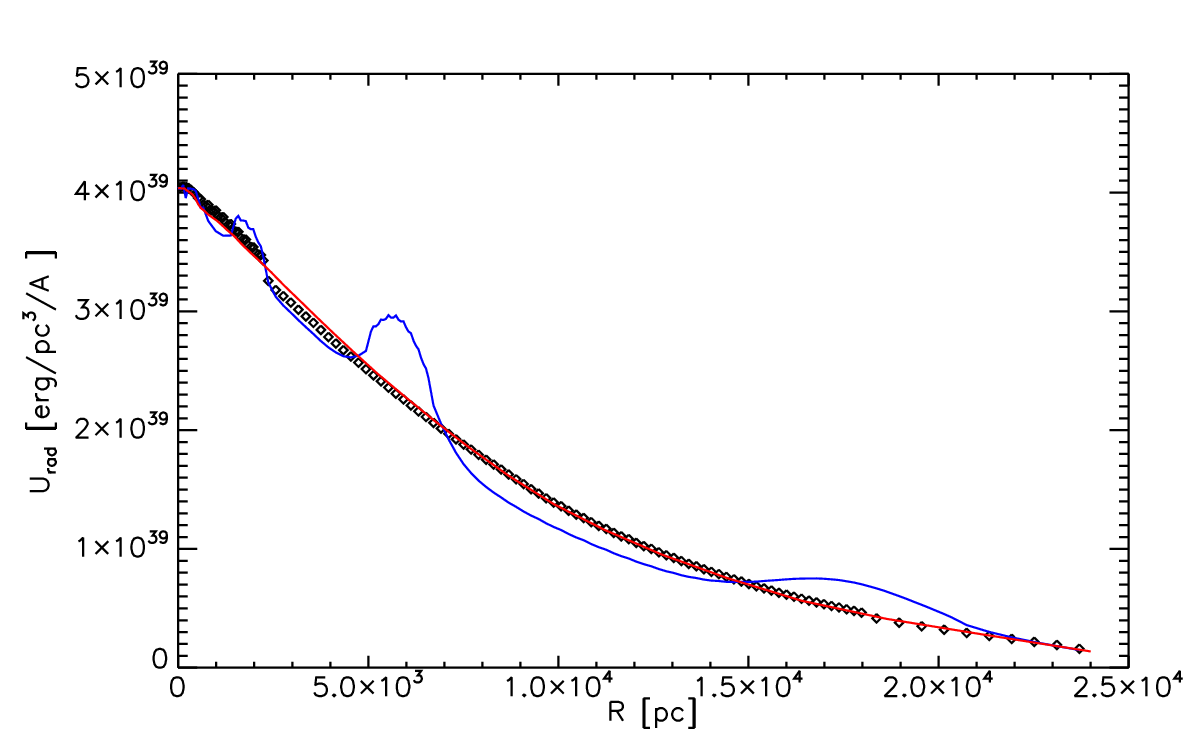
7 Summary and Outlook
In this paper we present a new ray-tracing dust radiation transfer algorithm which is able to handle arbitrary 3D geometries and
it is specifically designed to calculate accurate RFED within galaxy models. The main optimization characteristics of this algorithm are
the following:
1) an adaptive 3D grid (see §3.1)
2) a ray-tracing algorithm based on the pre-calculation of a lower limit for the RFED (see §3.2 and §3.3)
3) an iterative procedure for the optimization of the angular density for the rays departing from each emitting cell (§3.3).
Furthermore, parallelized versions of the code have been written for its use on shared-memory machines and computer clusters.
In order to verify the code accuracy, we performed comparisons with the results provided by other codes. Specifically, we used our code to calculate solutions for a spherical dusty shell illuminated by a central point source and for an axis symmetric galaxy model. For the first configuration, we considered as benchmark a set of solutions calculated by using the DUSTY 1D code (Ivezic & Elitzur 1997). We showed that the equilibrium dust temperature radial profiles and the outgoing flux spectra derived by our 3D calculations agree within a few percent with the benchmark solutions for models with low radial optical depths () but present larger discrepancies for more optically thick models (). The residual discrepancies, especially for the models with higher optical depths, are most probably due to the lack of dust self-heating in our code and the lower spatial resolution of the 3D calculations compared to the 1D ones. Since the geometry of the source emission/opacity of star/dust shell does not reproduce that for which our algorithm was developed, namely that of an extended distribution of stellar emission and dust, we also used a second benchmark. Thus, we considered the 2D calculations by Popescu et al. (2011) for the RFED distribution within their galaxy model. We calculated the contribution to the RFED distribution due to an old stellar disc and a young stellar disc separately and we compared the results for radial and vertical RFED profiles derived for a set of reference radii and vertical distances. We found a general good agreement between the 3D and 2D calculations within a few percent in most of the cases. At least part of the residual discrepancy can be accounted by the relatively low spatial resolution of the grid used in the 3D calculation, which is not sufficient to properly resolve the thin disc component of the galaxy model of Popescu et al. (2011). We showed an example of a 3D application of the code by performing RT for a spiral galaxy model where in one case the emissivity of the young stellar population and associated dust opacity are distributed in logarithmic spiral arms and in another case are distributed in exponential discs. We found that the edge-on images, the attenuation as a function of inclination and the azimuthally average RFED profiles on the galaxy plane are approximately the same for the two models. This suggests that the spatially integrated SEDs of spirals can be well described by 2D models.
The tests we performed have shown that, in the conditions where dust self-heating is negligible and
the 3D spatial resolution is high enough to resolve emission and opacity distributions, our code can be used to calculate
accurate solutions for the RFED. This characteristic is particularly important for the calculation of stochastically heated dust
emission, which requires both the overall intensity and the colour of the radiation field to be calculated in an accurate way.
In a future work we will show applications of the code for the calculation of infrared emission. This will be performed using our 3D
RT code coupled with the dust emission code used by Popescu et al. (2011), which
self-consistently calculates the stochastic emission from small grains and PAH molecules. In this way, it will be possible to use our
code to obtain both integrated
SEDs and images in the mid- and fir-infrared for galaxies with arbitrary geometries.
In addition, an important step will be to further optimize the code in order to make it possible to run on grids containing millions of
cells in a reasonably short time. This will allow us to
improve further the accuracy of the calculation for RFED within multi-scale structures spanning at least three orders of
magnitude, such as from pc to 10 kpc in the case of a galaxy ISM.
Acknowledgements
We acknowledge support from the UK Science and Technology Facilities Council (STFC; grant ST/J001341/1). GN thanks S. Dalla, K. Foyle, E. Kafexhiu, T. Laitinen, J. Steinacker for useful suggestions and/or discussions. CCP thanks the Max Planck Institute für Kernphysik for support during a sabbatical, when this work was completed.
References
- Abel & Wandelt (2002) Abel, T., Wandelt, B. D. 2002, MNRAS, 330, 53
- Baes et al. (2011) Baes, M., Verstappen, J., De Looze, I., Fritz, J., Saftly, W. et al. 2011, ApJS, 196, 22
- Bendo et al. (2012) Bendo, G. J., Boselli, A., Dariush, A., Pohlen, M., Roussel, H. et al. 2012, MNRAS, 419, 1833
- Bianchi et al. (1996) Bianchi, S., Ferrara, A., Giovanardi, C. 1996, ApJ, 465, 127
- Bianchi et al. (2008) Bianchi, S. 2008, A&A, 490, 461
- Bisbas et al. (2012) Bisbas, T. G., Bell, T. A., Viti, S., Yates, J., Barlow, M. J. 2012, MNRAS, 427, 2100
- Chakrabarti et al. (2009) Chakrabarti, S., Whitney, B. A. 2009, ApJ, 690, 1432
- Dale et al. (2007) Dale, D. A., Gil de Paz, A., Gordon, K. D., Hanson, H. M., Armus, L., Bendo, G. J. et al. 2007, ApJ, 655, 863
- Dale et al. (2012) Dale, D. A., Aniano, G., Engelbracht, C. W., Hinz, J. L., Krause, O. et al. 2012, ApJ, 745, 95
- Draine & Li (2007) Draine, B. T., Li, A. 2007, ApJ, 657, 810
- Driver et al. (2007) Driver, S. P., Popescu, C. C., Tuffs, R. J., Liske, J., Graham, A. W. 2007, MNRAS, 379, 1022
- Driver et al. (2008) Driver, S. P., Popescu, C. C., Tuffs, R. J., Graham, A. W. et al. 2008, ApJ, 678, 101
- Driver et al. (2012) Driver, S. P., Robotham, A. S. G., Kelvin, L., Alpaslan, M., Baldry, I. K. et al. 2012, MNRAS, 427, 3244
- Dullemond & Turolla (2000) Dullemond, C. P., Turolla, R. 2000, A&A, 360, 1187
- Efstathiou & Rowan-Robinson (1990) Efstathiou, A., Rowan-Robinson, M. 1990, MNRAS, 245, 275
- Ercolano et al. (2005) Ercolano, B., Barlow, M. J., Storey, P. J., 2005, MNRAS, 362, 1038
- Fischer et al. (1994) Fischer, O., Henning, Th., Yorke, H. W. 1994, A&A, 284, 187
- Gordon et al. (2001) Gordon, K. D., Misselt, K. A., Witt, Adolf N., Clayton, Geoffrey C. 2001, ApJ, 551, 269
- Górski et al. (2005) Górski, K. M., Hivon, E., Banday, A. J., Wandelt, B. D., Hansen, F. K., et al. 2005, ApJ, 622, 759
- Grootes et al. (2013) Grootes, M. W., Tuffs, R. J., Popescu, C. C., Pastrav, B., Andrae, E. et al. 2013, ApJ, 766, 59
- Guhathakurta & Draine (1989) Guhathakurta, P., Draine, B. T.,1989, ApJ, 345, 230
- Gunawardhana et al. (2011) Gunawardhana, M. L. P., Hopkins, A. M., Sharp, R. G., Brough, S., Taylor, E. et al. 2011, MNRAS, 415, 1647
- Hummer & Rybicki (1971) Hummer, D. G., Rybicki, G. B. 1971, MNRAS, 152, 1
- Ivezic & Elitzur (1997) Ivezic, Z., Elitzur, M. 1997, MNRAS, 287, 799
- Ivezic et al. (1997) Ivezic, Z., Groenewegen, M. A. T., Men’shchikov, A., Szczerba, R. 1997, MNRAS, 291, 121
- Jonsson (2006) Jonsson, P. 2006, MNRAS, 372, 2
- Kylafis & Bahcall (1987) Kylafis, N. D., Bahcall, J. N. 1987, ApJ, 317, 637
- Kuiper et al. (2010) Kuiper, R., Klahr, H., Dullemond, C., Kley, W.; Henning, T. 2010, A&A, 511, 81
- Mattila (1970) Mattila, K. 1970, A&A, 9, 53
- Misiriotis et al. (2001) Misiriotis, A., Popescu, C. C., Tuffs, R., Kylafis, N. D. 2001, A&A, 372, 775
- Misiriotis et al. (2000) Misiriotis, A., Kylafis, N. D., Papamastorakis, J., Xilouris, E. M. 2000, A&A, 353, 117
- Odenwald et al. (1998) Odenwald, S., Newmark, J., Smoot, G. 1998, ApJ, 500, 554O
- Pascucci et al. (2004) Pascucci, I., Wolf, S., Steinacker, J., Dullemond, C. P., Henning, Th., et al. 2004, A&A, 417, 793
- Popescu et al. (2000) Popescu, C. C., Misiriotis, A., Kylafis, N. D., Tuffs, R. J., Fischera, J. 2000, A&A, 362, 138
- Popescu & Tuffs (2002) Popescu, C. C., Tuffs, R. J. 2002, MNRAS, 335, 41
- Popescu et al. (2002) Popescu, C. C., Tuffs, R. J., Völk, H. J., Pierini, D., Madore, B. F. 2002, ApJ, 567, 221
- Popescu et al. (2011) Popescu, C. C., Tuffs, R. J., Dopita, M. A., Fischera, J., Kylafis, N. D., Madore, B. F. 2011, A&A, 756, 138
- Popescu & Tuffs (2013) Popescu, C. C., Tuffs, R. J. 2013, MNRAS, 436, 1302
- Roark et al. (1974) Roark, T., Roark, B., Collins, G. W., II 1974, ApJ, 190, 67
- Robitaille (2011) Robitaille, T. P. 2011, A&A, 536, 79
- Rowan-Robinson (1980) Rowan-Robinson, M. 1980, ApJS, 44, 403
- Schechtman-Rook et al. (2012) Schechtman-Rook, A., Bershady, M, A., Wood, K. 2012, ApJ, 746, 70
- Semionov & Vansevic̆ius (2005) Semionov, D., Vansevic̆ius, V. 2005, BaltA, 14, 543
- Semionov & Vansevic̆ius (2006) Semionov, D., Vansevic̆ius, V. 2006, BaltA, 15, 601
- Semionov et al. (2006) Semionov, D., Kodaira, K., Stonkutė, R., Vansevičius, V. 2006, BaltA, 15, 581
- Siebenmorgen et al. (1992) Siebenmorgen, R., Kruegel, E., Mathis, J. S. 1992, A&A, 266, 501
- Silva et al. (2011) Silva, L., Schurer, A., Granato, G. L., Almeida, C., Baugh, C. M. et al. 2011, MNRAS, 410, 2043
- Sodroski et al. (1997) Sodroski, T. J., Odegard, N., Arendt, R. G., Dwek, E., Weiland, J. L., Hauser, M. G., Kelsall, T. 1997, ApJ, 480, 173
- Steinacker et al. (2003) Steinacker, J., Henning, T., Bacmann, A., Semenov, D. 2003, A&A, 401, 405S
- Steinacker et al. (2013) Steinacker, J., Baes, M., Gordon, K. 2013, arXiv1303.4998S
- Xilouris et al. (1998) Xilouris, E. M., Alton, P. B., Davies, J. I., Kylafis, N. D., Papamastorakis, J., Trewhella, M. 1998, A&A, 331, 894
- Xilouris et al. (1999) Xilouris, E. M., Byun, Y. I., Kylafis, N. D., Paleologou, E. V., Papamastorakis, J. 1999, A&A, 344, 868
- Xilouris et al. (1997) Xilouris, E. M., Kylafis, N. D., Papamastorakis, J., Paleologou, E. V., Haerendel, G. 1997, A&A, 325, 135
- Weingarner & Draine (2001) Weingartner, J. C., Draine, B. T. 2001, ApJ, 548, 296
- Witt (1977) Witt, A. N. 1977, ApJS, 35, 1
- Witt (1996) Witt, A. N., Gordon, K. D. 1996, ApJ, 463, 681
- Witt & Stephans (1974) Witt, A. N., Stephens, T. C. 1974, AJ, 79, 948
- Witt et al. (1992) Witt, A. N., Thronson, H. A., Jr., Capuano, J. M., Jr. 1992, ApJ, 393, 611