Interpolation and Approximation of Polynomials in Finite Fields over a Short Interval from Noisy Values
Abstract.
Motivated by a recently introduced HIMMO key distribution scheme, we consider a modification of the noisy polynomial interpolation problem of recovering an unknown polynomial from approximate values of the residues of modulo a prime at polynomially many points taken from a short interval.
Key words and phrases:
Noisy polynomial interpolation, finite fields, lattice reduction, HIMMO key distribution scheme1. Introduction
1.1. Motivation
Here, we consider the following problem:
Given a prime , recover an unknown polynomial over a finite field of elements from several approximations to the values , computed at several points .
Several problems of this type are related to the so-called hidden number problem introduced by Boneh and Venkatesan [2, 3], and have already been studied intensively due to their cryptographic relevance, see the survey [26].
Usually the evaluation points are chosen from the whole field . However, here, motivated by the links and possible applications to the recently introduced HIMMO key distribution scheme [8], we concentrate on a very different case, which has never been discussed in the literature. Namely, in the settings relevant to HIMMO, the values of are taken from a short interval rather than from the whole field . This case requires a careful adaptation of existing algorithms of [25, 27] and also establishing new number theoretic results about the frequency of small residues of polynomial values evaluated at a small argument, which are based on some ideas from [4, 5].
We remark the polynomial recovery problem as studied in this paper arises in a collusion attack on a single node in the HIMMO system. Collusion attacks on the complete HIMMO system lead to recovery problems involving several polynomials reduced modulo several distinct unknown integers, which we believe to be much more difficult.
1.2. Polynomial noisy interpolation and approximation problems
For a prime we denote by the field of elements. We identify the elements of with the set , so we can talk about their bits (for example most and least significant bits) and also approximations.
We consider the noisy polynomial interpolation problem of finding an unknown polynomial
of degree from approximations to values of (treated as elements of the set ) at polynomially many points selected uniformly at random.
More precisely, for integers and we denote by the distance between and the closest multiple of , that is,
Then, these approximations can, for example, be given as integers with
| (1) |
for some “precision” for values of that are chosen uniformly at random from a certain set of “samples”.
In cryptographic applications, the approximations are usually given by strings of most or least significant bits of , where, if necessary, some leading zeros are added to make sure that is represented by bits, where is the bit length of .
It is clear that giving the most significant bits is essentially equivalent to giving approximations of the type (1) with an appropriate . We now observe that giving the least significant bits can be recast as a question of this type as well. Indeed, assume we are given some -bit integer so that
for some (unknown) integer . We now have so, if is the multiplicative inverse of in then, setting , we obtain an inequality of the type (1) with the polynomial instead of and .
So from now on we concentrate on the case where the approximations to are given in the form of (1).
The case of linear polynomials corresponds to the hidden number problem introduced by Boneh and Venkatesan [2, 3]. The case of general polynomials, including sparse polynomials of very large degree, has been studied in [25, 27] (see also [26] for a survey of several other problems of similar types). We note that if the polynomial belongs to some family of polynomials (such as polynomials of degree or sparse polynomials with monomials), it is crucial for the algorithms of [25, 27] to have some uniformity results for every non-zero polynomial of on the values of chosen uniformly at random from . We also note that a multiplicative analogue of this problem has been studied in [9].
We recall that in the settings of all previous works, typically the set is the whole field . In turn, this enables the use of such a powerful number theoretic technique as the method of exponential sums and thus the use of the Weil bound (see [17, Theorem 5.38]) for dense polynomials and the bound of Cochrane, Pinner and Rosenhouse [6] for sparse polynomials. In particular, in [27] a polynomial time algorithm is designed that works with very large values of , namely, up to , provided that is a sparse polynomial of degree and with monomials (of known degrees), where is some absolute constant. The analysis of the algorithm of [27] is based on the method of exponential sums, the bound of [6] and some ideas related to the Waring problem.
We also note that if is an interval of length at least for some fixed , where, as before , then one can use the method of [25, 27] augmented with the bounds of exponential sums obtained via the method of Vinogradov, see the striking results of Wooley [28, 29, 30]. However, here we are interested in shorter intervals of the form
which appear naturally in the construction of [8]. Thus instead of the method of exponential sums, we use some ideas from [4, 5].
We remark that for the noisy interpolation to succeed, we always assume that some low order the coefficients of are known, where is such that for some fixed . Clearly such a condition is necessary as if then the approximations of the type (1) are not likely to be sufficient to distinguish between
from approximations (1) at random . Furthermore, it is clear that without loss of generality we can always assume that
Note that in the case when the test set is the whole field we only need to request that the constant coefficient of is known (which is also, always assumed to be zero, see [2, 3, 25, 27]).
The above example, which shows the limits of interpolation of from the information given by (1), motivates the following question of approximation to , which is also more relevant to attacking HIMMO. Namely, instead of finding a polynomial we ask whether we can find a polynomial , such that and are close to each other for all so the approximations (1) do not allow to distinguish between and . In the terminology of [8] both and lead to the same keys and thus the attacker can use instead of .
Finally, we note that the algorithmic problems considered in this paper have led us to some new problems which are of intrinsic number theoretic interest.
1.3. Approach and structure
Generally, our approach follows that of [25, 27] which in turn is based on the idea of Boneh and Venkatesan [2, 3]. Thus lattice algorithms, namely the algorithm for the closest vector problem, see Section 3.1, and a link between this problem and polynomial approximations, see Section 3.2, play a crucial role in our approach.
However, the analysis of our algorithm requires very different tools compared with those used in [25, 27]. Namely we need to establish some results about the frequency of small polynomial values at small arguments, which we derive in Section 2.1, closely following some ideas from [4, 5].
It also clear that there is a natural limit for such estimates on the frequency of small values as any polynomial with small coefficients takes small values at small arguments (it is certainly easy to quantify the notion of “small” in this statement). In fact our bound of Lemma 1 is nontrivial up to exactly this limit.
Rather unexpectently, in Section 2.2 we show that there are several other types of polynomials which satisfy this property: that is, they take small values at small arguments even if the coefficients are quite large (certainly this may only happen beyond the range of the bound of Lemma 1 which applies to all polynomials).
We call such polynomials exceptional. Then, after recalling in Section 2.3 some result from analytic number theory, in Section 2.4 we give some results describing the structure of the coefficients of exceptional polynomials. Note the presence of exceptional polynomials makes noisy polynomial interpolation impossible for a wide class of instances (which is actually good news for the security of HIMMO). So it is important to understand the structure and the frequency of exceptional polynomials. The results of Section 2.4 provide some partial progress toward this goal, yet many important questions are still widely open.
Our main results are presented in Sections 4.1 and 6. In Section 4.1 we treat the noisy polynomial interpolation problem, where we actually want to recover the hidden polynomial . However, from the cryptographic point of view it is enough to recover another polynomial which for all or most of small arguments takes values close to those taken by . Here the existence of exceptional polynomials becomes of primal importance. We use the results of Section 2.4 to obtain an upper bound on the number of such polynomials .
Furthermore, in Sections 5.1 and 5.2 we also give two interesting explicit constructions of such exceptional polynomials, which we illustrate by some concrete numerical examples.
In Section 6 we treat the approximate recovery problem and give a formula that predicts whether an approximate recovery is likely to be successful, depending on the number of randomly chosen observation points. We compare its predictions with numerical experiments for parameter values suitable for HIMMO.
1.4. Notation
Throughout the paper, the implied constants in the symbols ‘’, ‘’ and ‘’ may occasionally, where obvious, depend on the degrees of the polynomials involved and on the real parameter and are absolute, otherwise. We recall that the notations , and are all equivalent to the assertion that the inequality holds for some constant .
The letter always denotes a prime number, while the letters , , , and (in lower and upper cases) always denote positive integer numbers.
2. Distribution of Values of Polynomials
2.1. Polynomial values in a given interval
For a polynomial
and two intervals
of and consecutive integers, respectively, we denote by the number of values for which (where the elements of the intervals and are embedded into under the natural reduction modulo ).
For two intervals and of the same length, various bounds on are given in [4, 5]. It is easy to see that the argument of the proof of [5, Theorem 1] allows us to estimate for intervals of and of different lengths as well.
To present this result, for positive integers , and , we denote by the number of solutions to the system of equations
with
Next, we define as the smallest integer such that for there exists a constant depending only on and and such that
holds as . Presently, the strongest available upper bound
is due to Wooley [30], see also [29, Theorem 1.1] and [28, Theorem 1.1]; note that, in particular, these bounds also imply the existence of which is a very nontrivial fact.
It is now easy to see that the proof of [5, Theorem 1] can be generalised to lead to the following bound.
Lemma 1.
Let be a polynomial of degree . Then for intervals and with we have
as .
Note that Kerr [15, Theorem 3.1] gives a more general form of Lemma 1 that applies to multivariate polynomials and also to congruences modulo a composite number.
We also note, that several other results from [4, 5] can be extended from the case to the general case as well, but this does not affect our main result.
Clearly the bound of Lemma 1 is nontrivial provided that and also for a fixed and a sufficiently large . It is easy to see that this conditions cannot be substantially improved as it is clear that if then for any polynomial . Also, if then for , and . The above example may suggest that unless the coefficients of are small, the value of can be nontrivially estimated even for . We now show that this is false and in fact there are many other polynomials, which we call exceptional, which have the same property.
2.2. Exceptional polynomials
Let us fix integers , , and . We now consider a polynomial
where
| (2) |
In particular for some integers
Then for with an integer we have
Hence for such values of , which implies the inequality for the above example. Taking to be small, we see that has quite large coefficients, however no nontrivial bound on is possible for .
In fact, in Sections 5.1 and 5.2 we give examples of polynomials with large coefficients that remain small for all small values of the arguments, that is, polynomials for which , for some rather short intervals compared with the length of .
In the above examples, the ratios of the coefficients and are chosen to be very close to rational numbers with small numerators and denominators. Alternatively, this can be written as the condition that the coefficients of satisfy
for some small integers , .
Below we present several results that demonstrate that this property indeed captures the class of exceptional polynomials with large values of adequately, at least in the qualitative sense.
First we need to recall some number theoretic results.
2.3. Some preparations
The following result is well-known and can be found, for example, in [20, Chapter 1, Theorem 1] (which is a more precise form of the celebrated Erdős–Turán inequality).
Lemma 2.
Let be a sequence of points of the unit interval . Then for any integer , and an interval , we have
To use Lemma 2 we also need an estimate on exponential sums with polynomials, which is essentially due to Weyl, see [14, Proposition 8.2].
Let denote the distance between a real and the closest integer (which can be considered as a modulo 1 version of the notation ).
Lemma 3.
Let be a polynomial of degree with the leading coefficient . Then
Finally, we need the following version of several similar and well known inequalities, see, for example, [14, Section 8.2].
Lemma 4.
For any integers , , and with
and a real with
we have
Proof.
First we estimate the contribution from trivially as . For the remaining we note that
as
Therefore, the contribution from can be estimated as
Since and this simplifies as
which concludes the proof.
2.4. Coefficients of exceptional polynomials
Our first result uses in an essential way the argument of the proof of [5, Theorem 3],
Lemma 5.
Let
be a polynomial of degree . Assume that for some and intervals and with we have
Then
for some integers
Proof.
As we have mentioned, we follow the proof of [5, Theorem 3].
Let . Since , there exist pairs such that lie in an interval of length and .
Now, we consider the system of congruences
The determinant of this system is the determinant of a Vandermonde matrix:
Note that . Thus, we have that
| (3) |
where
| (4) |
and is the determinant of the matrix obtained from the Vandermonde matrix after removing the -th row and the -th column, , .
It is easy to see that for each , the determinant is a polynomial in variables , , , of degree , which vanishes when for distinct and . Thus
where is a polynomial (that does not depend on or ) of degree . Therefore, we have
This estimate and (4) together imply the bound
| (5) |
On the other hand, it is clear that
| (6) |
We note that if and are fixed the expressions given by the example (2) and those of Lemma 5 differ by a factor and it is certainly natural to try to reduce this gap.
We now obtain yet another estimate on that depends only on the behaviour of the leading coefficient.
We recall the definition of used in Lemma 1. Since for we can use the bound of Lemma 1, we assume that
| (7) |
Then the argument of the proof of [4, Theorem 5] leads to the following result:
Lemma 6.
Let
be a polynomial of degree . Assume that for some and intervals and with satisfying (7) we have
Then either
or
for some integer
Proof.
Let . We apply Lemma 2 to the sequence of fractional parts , , with
Without loss of generality, we can assume that as otherwise the bound is trivial. Then we have and thus
for , we derive
Therefore, by Lemma 3, we have
Now, separating from the sum over the terms with , (giving a total contribution ), we obtain
| (8) |
where
Hence, recalling the choice of , we derive
| (9) |
The Hölder inequality implies the bound
Collecting together the terms with the same value of
and using the well-known bound on the divisor function, we conclude that
Let us set Note that our assumption (7) implies that.
By the Dirichlet approximation theorem we can write
for some integers and . Note that this immediately implies that . Hence
for some integer with
It now remains to estimate or .
Note that the dependence on in the bound on of Lemma 6 is worse that that of Lemma 5. However, since we are mostly interested in large values of , for example, the extreme case is of special interest, Lemma 6 limits the possible values of as , which is stricter than the bound that follows from the estimates of Lemma 5 on and .
3. Lattices and Polynomials
3.1. Background on lattices
As in [2, 3], and then in [25, 27], our results rely on some lattice algorithms. We therefore review some relevant results and definitions, we refer to [7, 10, 11] for more details and the general theory.
Let be a set of linearly independent vectors in . The set of vectors
is called an -dimensional full rank lattice.
The set is called a basis of .
The volume of the parallelepiped defined by the vectors is called the volume of the lattice and denoted by . Typically, lattice problems are easier when the Euclidean norms of all basis vectors are close to .
One of the most fundamental problems in this area is the closest vector problem, CVP: given a basis of a lattice in and a target vector , find a lattice vector which minimizes the Euclidean norm among all lattice vectors. It is well know that CVP is NP-hard when the dimension (see [21, 22, 23, 24] for references).
However, its approximate version admits a deterministic polynomial time algorithm which goes back to the lattice basis reduction algorithm of Lenstra, Lenstra and Lovász [16], see also [21, 22, 23, 24] for possible improvements and further references.
We remark that all lattices that appear in this paper are of fixed dimension, so instead of using the above approximate CVP algorithms, we can simply use the following result of Micciancio and Voulgaris [19].
Let denote the standard Euclidean norm in .
Lemma 7.
For any fixed , there exists a deterministic algorithm which, for given a lattice generated by an integer vectors
and a vector , in time polynomial in
finds a lattice vector satisfying
3.2. Lattices and polynomial approximations
For , integer , we set and we denote by the -dimensional lattice generated by the rows of the following -matrix
| (10) |
The following result is a generalization of several previous results of similar flavour, see [2, 25, 27].
Lemma 8.
Let be fixed and let be a sufficiently large prime. Assume that some real numbers and integer numbers , satisfy
Then there is an integer , depending only on and , such that if
and are chosen uniformly and independently at random, then with probability at least the following holds. For any vector with
all vectors
satisfying
| (11) |
are of the form
Proof.
Let denote the set of polynomials
| (12) |
with .
We see from Lemma 1 (taking into account that is a monotonically non-decreasing function of ) that for any polynomial the probability that
for selected uniformly at random is
provided that is large enough, where depends only on and .
Therefore, for any ,
where the probability is taken over chosen uniformly and independently at random.
Since , we obtain
for , provided that is large enough.
We now fix some integers with
| (13) |
Let be a lattice point satisfying (11).
Clearly, for a vector , there are some integer such that
Now, if , , then for all we have
since otherwise there is such that and thus , which contradicts (11) again. Hence is of the desired form.
As we have seen, the condition (13) holds with probability exceeding and the result follows.
4. Main Results
4.1. Polynomial interpolation problem
We are ready to prove the main result. We follow the same arguments as in the proof of [2, Theorem 1] that have also been used for several other similar problems, see [25, 26, 27].
Theorem 9.
Let be fixed and let be a sufficiently large prime. Assume that a real and integers , satisfy
There exists an integer , depending only on and and a deterministic polynomial time algorithm such that for any polynomial
given integers and with
its output satisfies
if are chosen uniformly and independently at random from .
4.2. Polynomial approximation problem
As we have mentioned, it is impossible to recover a “complete” polynomial of degree from the approximations (1) for for a small value of . However, it is interesting to estimate the number of possible “false” candidates , which for many take values close to those of .
Namely, for a polynomial , and real positive parameter we define as the set of polynomials with
for at least values of . For example, if for some fixed we have
the by Lemma 1 we have unless . So we now consider slightly smaller values of .
Theorem 10.
Let be fixed and let be a sufficiently large prime. Assume real and integers , satisfy
for some fixed . Then for we have
Proof.
The case of , when the recovery of from the approximations (1) with is impossible regardless of the number of queries and the complexity of algorithm is certainly of special interest. We denote .
Under the conditions of and of Theorem 10 we have
Clearly if the coefficients of are sufficiently close to those of then . This argument easily leads to the lower bound
We now show that this is not necessary and in particular the set contains many polynomials that “visually” look very differently from .
5. Constructions of Exceptional Polynomials
5.1. Flat polynomials
Let us take any integer and non-zero polynomial of degree and with coefficients in the range such that
For examples if is a square-free integer, we can construct such a polynomial via the Chinese Remainder Theorem from polynomials of the form for each prime divisor .
Alternatively, given an integer , for any with
| (15) |
one can consider take with an integer that is relatively prime to . We note that the function , defined as the smallest with the property (15) is called the Smarandache function and has been extensively studied in the literature, see [13] and references therein.
Now, for any sufficiently small integers we define the coefficients from the congruences , , and consider the polynomial
It is easy to see that the coefficients of can be rather large compared to . Furthermore, for every as the fractions , , take integer values of size , we have
where
Varying the parameter , the polynomials and the integers , , (and also introducing a small non-zero constant coefficient ) one can get a large family of such polynomials that remain “flat” on short intervals. In particular, one can choose to be a product of many small primes. This argument can easily be made more precise with explicit constants, however we instead present an illustrative example of such a polynomial.
Let us fix the prime
| (16) |
We also set , and for , choose integers such that :
and pick numbers randomly such that , for example:
and let
The plot on Figure 1, shows that (where is indicated by the horizontal line) for :
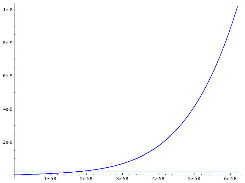
.
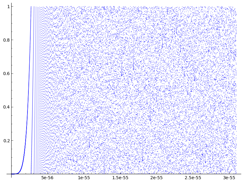
The plot in Figure 2 shows that stays flat and close to zero for close to 0 and, after some transition period, appears to behave completely randomly for .
5.2. Oscillating polynomials
A different type of polynomial with large coefficients that is small in an interval can be constructed if . Thus this class is interesting only if the degree becomes a growing parameter, which is actually the case in the settings of HIMMO.
Let be polynomial of degree that, after reduction modulo takes values in the interval for . This means that
for integer valued functions and , where for , .
Let denote the discrete difference operator, that is, for any function , . We have, since is a polynomial of degree :
so . On the other hand, since for , it holds that for . For it follows that for all , so that after -fold integration we have
This means that and are both polynomials of degree at most on the interval .
For there are more possibilities. For instance, if
we obtain, by integrating
Defining
and
we have a decomposition , where, for integer , these three functions are integer valued. By choosing to be close to and, for , close to the residues of modulo , we obtain a polynomial of degree that, after reduction modulo , lies in for arguments in the interval . For the prime given by (16), with , and
where denotes the closest integer (and defined arbitrary in case of a tie), we obtain the graph in Figure 3. Note that the left part of the graph in Figure 3 looks like a plot of two curves, while in fact this is one curve, which exhibits a highly oscillatory behaviour.

.
6. Approximate recovery
6.1. Approach
Using lattice reduction and rounding techniques, we are able to find a polynomial satisfying for , the set of observation points. The question is whether approximates also in all or at least some, non-observed points . The lattice used in this technique is spanned by the rows of
where the first columns correspond to the evaluation of the polynomial in the points , and the last columns to its coefficients, scaled such that all coordinates of the wanted lattice point lie in an interval of length . In the remainder of this section we focus on the first columns, that is, the -dimensional lattice of which the rows of the matrix
are an overcomplete basis.
If , a straightforward basis transformation that corresponds to Lagrange interpolation on eliminates rows and transforms this basis into
from which it is clear that (see Section 3.1 for the definition of ).
We consider the case that , so that, as shown in Section 5.2 all functions for which for all satisfy
for sufficiently small . These differences correspond to the -dimensional lattice in of which the rows of the matrix
form a basis. The volume of the lattice corresponding to these approximating polynomials is given by
The determinant can be expanded as a sum of squares of Vandermonde determinants, yielding
where the set runs over all subsets of with elements.
The lattice technique returns a polynomial such that the point
lies in the lattice . If this pointis also a lattice point of , then approximates in all points of , and the attack succeeds. So, from the attacker point of view, it is good if all lattice vectors of that do not lie in are long, that is, have the infinity norm greater than , since then those points lie outside the hypercube around the target vector.
We define the lattice , obtained by orthogonally projecting all points of onto the hyperplane through the origin that is orthogonal to the basis vectors of . Obviously it holds that
If does not have short vectors, its volume is large and the attack succeeds. If its volume is small, has short vectors and, depending on the number of independent short vectors and their lengths, the attack is likely to fail.
This leads us to define the function
It compares an esimate of the length of the shortest vector in , based on the Minkowski bound, to , in an average sense. The cross-over between having short vectors or not is at .
The factor in the definition of the function is included to account for the orientations of and of with respect to the coordinate axes, and the averaging is done in such a way that it can be explicitly evaluated if is much smaller that but is not too small:
The integral of the square of the Vandermonde determinant is equal to times the determinant of the Hilbert matrix , which has been calculated by Hilbert himself [12] and is equal to
We thus obtain
| (17) |
6.2. Tests
We are mainly interested in parameter values corresponding to HIMMO, that is, when we have a polynomial of degree and -bit keys, we choose to have precisely bits and let . We are interested only in reconstruction in intervals of length at most . Note that in this case becomes independent of .
Figure 4 shows the reconstriction error versus for a randomly chosen polynomial of degree , , a random 112-bit prime and and , respectively. The observation points are uniformly chosen in the interval . For , the error appears to be random for all , whereas for the error is close to for small .


Figure 5 shows graph of as a function of , showing that becomes positive at . This suggests that an approximate reconstruction is likely to be successful for , completely in line with our experimental results.

For larger degree , and , a -bit prime, , the function becomes positive for , which may be too large for a successful lattice attack on the present computers. But in a shorter interval, , the function becomes positive at , see Figure 6.

The experimental results in Figures 7, 8 and 9 show how the reconstruction improves as increases from to . For , the reconstruction is close to zero only in the observation points (note that the points near the horizontal line are also considered to be close to zero). For also in a sizeable fraction of the not-observed points. Finally for in nearly all points of an interval of length .


Finally, we note that for fairly small values of , for example, , is negative for all if is large enough, as shown for in Figure 10. This suggests that approximate reconstruction in the full interval cannot work, no matter how many observation points are used.

7. Comments
Clearly in practical implementations of our algorithm, using a certain approximate version of Lemma 7 is more natural. One can easily check that the algorithm and the result of Theorem 9 remain valid in this case as well.
In the settings of HIMMO with -bit keys and -bit identifiers we have , and , see [8], so Theorem 9 does not apply. This can be considered as an indirect confirmation of the strength of HIMMO: recovery of the complete polynomial is impossible.
From studying (17) as a function of for various values of , we can obtain indications if an approximate recovery in an interval is likely to succeed, also for shorter intervals, , that do not contain all possible identifiers.
We also recall that there is a different approach to the hidden number problem, due to Akavia [1]. This approach does not use any lattice algorithms but rather examine the Fourier coefficients of the “hidden” linear function. However, the properties of these coefficients (large values near the origin and a smooth decay away from the origin) do not hold for non-linear polynomial functions, where all Fourier coefficients are expected to be of about the same size.
References
- [1] A. Akavia, ‘Solving hidden number problem with one bit oracle and advice’, Lect. Notes in Comp. Sci., Springer-Verlag, Berlin, 5677 (2010), 337–354.
- [2] D. Boneh and R. Venkatesan, ‘Hardness of computing the most significant bits of secret keys in Diffie–Hellman and related schemes’, Lect. Notes in Comp. Sci., Springer-Verlag, Berlin, 1109 (1996), 129–142.
- [3] D. Boneh and R. Venkatesan, ‘Rounding in lattices and its cryptographic applications’, Proc. 8th Annual ACM-SIAM Symp. on Discr. Algorithms, SIAM, 1997, 675–681.
- [4] M.-C. Chang, J. Cilleruelo, M. Z. Garaev, J. Hernández, I. E. Shparlinski and A. Zumalacárregui, ‘Points on curves in small boxes and applications’, Preprint, 2011 (available from http://arxiv.org/abs/1111.1543).
- [5] J. Cilleruelo, M. Z. Garaev, A. Ostafe and I. E. Shparlinski, ‘On the concentration of points of polynomial maps and applications’, Math. Zeit., 272 (2012), 825–837.
- [6] T. Cochrane, C. Pinner and J. Rosenhouse, ‘Bounds on exponential sums and the polynomial Waring’s problem ’, Proc. Lond. Math. Soc., 67 (2003), 319–336.
- [7] J. H. Conway and N. J. A. Sloane, Sphere packings, lattices and groups, 3rd edition. Grundlehren der Mathematischen Wissenschaften, vol. 290, Springer-Verlag, New York, 1999.
- [8] O. Garcia-Morchon, R. Rietman, L. Tolhuizen, D. Gómez-Pérez, J. Gutierrez and S. Merino del Pozo, ‘An ultra-lightweight ID-based pairwise key establishment scheme aiming at full collusion resistance’, ePrint Archive, Report 618, 2012 (available from http://eprint.iacr.org/2012/618).
- [9] J. von zur Gathen and I. E. Shparlinski, ‘Polynomial interpolation from multiples’, Proc. 15th ACM-SIAM Symposium on Discrete Algorithms, SIAM, 2004, 1125–1130.
- [10] M. Grötschel, L. Lovász and A. Schrijver, Geometric algorithms and combinatorial optimization, Algorithms and Combinatorics: Study and Research Texts, vol. 2, Springer-Verlag, Berlin, 1993.
- [11] P. M. Gruber and C. G. Lekkerkerker, ‘Geometry of numbers’, 2nd edition, North-Holland Mathematical Library, vol. 37. North-Holland Publishing Co., Amsterdam, 1987.
- [12] D. Hilbert, ‘Ein Beitrag zur Theorie des Legendre’schen Polynoms’, Acta Mathematica, 18 (1894), 155–-159.
- [13] A. Ivić, ‘On a problem of Erdős involving the largest prime factor of ’, Monatsh. Math., 145 (2005), 35–46.
- [14] H. Iwaniec and E. Kowalski, Analytic number theory, Amer. Math. Soc., Providence, RI, 2004.
- [15] B. Kerr, ‘Solutions to polynomial congruences in well shaped sets’, Bull. Aust. Math. Soc., 88 (2013), 435–447.
- [16] A. K. Lenstra, H. W. Lenstra and L. Lovász, ‘Factoring polynomials with rational coefficients’, Mathem. Ann., 261 (1982), 515–534.
- [17] R. Lidl and H. Niederreiter, Finite fields, Cambridge Univ. Press, Cambridge, 1997.
- [18] D. Micciancio, On the hardness of the shortest vector problem, PhD Thesis, MIT, 1998.
- [19] D. Micciancio and P. Voulgaris, ‘A deterministic single exponential time algorithm for most lattice problems based on Voronoi cell computations’, SIAM J. Comp., 42 (2013), 1364–1391.
- [20] H. L. Montgomery, Ten lectures on the interface between analytic number theory and harmonic analysis, Amer. Math. Soc., Providence, RI, 1994.
- [21] P. Q. Nguyen, ‘Public-key cryptanalysis’, Recent Trends in Cryptography, Contemp. Math., vol.477, Amer. Math. Soc., 2009, 67–119.
- [22] P. Q. Nguyen and J. Stern, ‘Lattice reduction in cryptology: An update’, Lect. Notes in Comp. Sci., Springer-Verlag, Berlin, 1838 (2000), 85–112.
- [23] P. Q. Nguyen and J. Stern, ‘The two faces of lattices in cryptology’, Lect. Notes in Comp. Sci., Springer-Verlag, Berlin, 2146 (2001), 146–180.
- [24] O. Regev, ‘On the complexity of lattice problems with polynomial approximation factors’, The LLL Algorithm:Surveys and Applications, Springer-Verlag, 2010, 475–496.
- [25] I. E. Shparlinski, ‘Sparse polynomial approximation in finite fields’, Proc. 33rd ACM Symp. on Theory of Comput., Crete, Greece, July 6-8, (2001), 209–215.
- [26] I. E. Shparlinski, ‘Playing “Hide-and-Seek” with numbers: The hidden number problem, lattices and exponential sums’, Proc. Symp. in Appl. Math., Amer. Math. Soc., Providence, RI, 62 (2005), 153–177.
- [27] I. E. Shparlinski and A. Winterhof, ‘Noisy interpolation of sparse polynomials in finite fields’, Appl. Algebra in Engin., Commun. and Computing, 16 (2005), 307–317.
- [28] T. D. Wooley, ‘Vinogradov’s mean value theorem via efficient congruencing’, Ann. Math., 175 (2012), 1575–1627.
- [29] T. D. Wooley, ‘Vinogradov’s mean value theorem via efficient congruencing, II’, Duke Math. J., 162 (2013), 673–730.
- [30] T. D. Wooley, ‘Multigrade efficient congruencing and Vinogradov’s mean value theorem’, Preprint, 2011 (available from http://arxiv.org/abs/1310.8447).