KIAS-P14011
Production of Stoponium at the LHC
Abstract
Although the Large Hadron Collider (LHC) has not observed supersymmetric (SUSY) partners of the Standard Model particles, their existence is not ruled out yet. One recently explored scenario in which there are light SUSY partners that have evaded current bounds from the LHC is that of a light long-lived stop quark. In this paper we consider light stop pair production at the LHC when the stop mass is between 200 and . If the stops are long-lived they can form a bound state, stoponium, which then undergoes two-body decays to Standard Model particles. By considering the near-threshold production of such a pair through the gluon-gluon fusion process and taking into account the strong Coulombic interactions responsible for the formation of this bound state, we obtain factorization theorems for the stop pair inclusive and differential production cross sections. We also perform a resummation of large threshold logarithms up to next-to-next-to-leading logarithmic accuracy using well-established renormalization group equations in an effective field theory methodology. These results are used to calculate the invariant mass distributions of two photons or two bosons coming from the decay of the stoponium at the LHC. For our choices of SUSY model parameters, the stoponium is not detectable above Standard Model backgrounds in or at , but will be visible with of accumulated data if its mass is below when the LHC runs at .
I Introduction
The Large Hadron Collider (LHC) has confirmed the existence of the Higgs boson. The next main objective of future searches is to discover what lies beyond the Standard Model (BSM). Supersymmetric (SUSY) extensions of the SM are among the most well-studied scenarios for BSM physics, and are mainly motivated by theoretical considerations (e.g., the hierarchy problem). Although the LHC has not found any signals of BSM physics so far, SUSY extensions of the SM are not ruled out yet. Among a variety of SUSY scenarios, the possibility of a light stop has received a lot of attention since it is naturally well motivated [1, 2, 3, 4, 5, 6, 7, 8, 9]. A light stop is generally expected in the minimal supersymmetric Standard Model (MSSM) due to a large positive Yukawa coupling term in the renormalization group equation for the stop mass and possibly large mixing term between left and right stops in the stop mass matrix. On top of that, there are other motivations for the light stop coming from cosmological considerations. First, a light stop with a mass that is a few tens of above the lightest SUSY particle can successfully account for the thermal relic density of dark matter [10]. Second, electroweak baryogenesis is possible in the MSSM with a light stop [11, 12, 13]. Recently, the authors of Ref. [14] have found that a light stop mass between 200 and (with several additional conditions) is consistent with the currently available experiment constraints such as the Higgs mass, , etc.
Collider experiments search for stop quarks decaying to a top quark and neutralino or bottom quark and chargino and if the stop is light enough that these decays are not kinematically allowed, then the bounds from these searches are not relevant and the stop quark is likely long-lived. See Refs. [15, 16, 17, 18] for light stop searches from stop decays to top quark and neutralino or bottom quark and chargino. This SUSY spectrum can be obtained if the bino and wino masses are comparable to the Higgsino mass term so that the lightest neutralino and chargino masses are not degenerate. If stops exist, they will be produced at the LHC mainly through gluon-gluon fusion, much like the main production channel of the SM Higgs boson. The stops can either be produced singly or in pairs. If pair produced, they can then form a bound state, stoponium, through the strong Coulomb interaction. This bound state can then undergo two-body decays to SM particles, and the bound state will appear as a resonance above the SM background for , , or , for example. In earlier work [19, 20], we showed that these are good channels in which to search for heavy BSM particles that are strongly interacting. In this work we apply the methodology of Refs. [19, 20] to stop pairs. For early work advocating searching for stoponium in the channel, see Refs. [21, 22].
Since the LHC is a hadronic machine where two protons collide at very high energies, the partons inside the hadrons will initiate a hard reaction responsible for the production of massive particles. To separate nonperturbative long-distance QCD effects from the calculable short-distance effects, we derive factorization theorems for the production process. These theorems clarify what is perturbatively calculable and what is the proper form of the relevant hadronic matrix elements to be determined from experiment (or a nonperturbative QCD calculation). In cases where such factorization theorems hold, one then needs to deal with large logarithms encountered in perturbative calculations. Such large logarithms exist because the production process is characterized by several widely separated scales and thus large logarithms of the ratios of these scales need to be resummed.
In this work we utilize the effective field theory approach to establish a factorization theorem for the production of massive stop pairs. This is done by constructing effective operators, at each relevant scale, that mediate the production reaction. In our work, the relevant theories are soft-collinear effective theory (SCET) [23, 24, 25] and heavy-scalar effective theory (HSET). The former describes the multiscale physics behind the production of the stop pair through the gluon-gluon fusion process. The factorization of the production process into hard, soft, and collinear parts allows us to implement the threshold resummation by solving the renormalization group equations for each of these parts. HSET describes the production of a slowly moving stop pair whose strong Coulomb interactions will bind the stop pair into the stoponium. The strong Coulomb interactions are resummed to all orders using the Coulomb Green’s function and including the finite width of the stoponium yields a resonant shape in the vicinity of the stoponium mass [26, 27]. For recent next-to-next-to-leading logarithmic (NNLL) resummed calculations of squark and gluino production, including the Coulomb Green’s function, see Ref. [28]. Threshold resummation of squark and gluino production in Mellin space has been calculated up to NNLL accuracy in Refs. [29, 30, 31, 32, 33, 34, 35]. NNLL resummation in momentum space for stop pair production was recently reported in Refs. [36, 37].
The factorization theorem obtained allows us to resum large logarithms when the stop pair is produced near the partonic threshold which is the kinematical range of interest once we assume a light stop mass and LHC energies. The accuracy of resummation depends on the knowledge we have of the perturbatively calculable anomalous dimensions and beta functions appearing in the formulas for the resummed cross section. In this work the resummation is performed up to NNLL accuracy. The phenomenological impact of resummation is discussed below.
Finally, we consider the decay rates of the stoponium bound state, denoted , in two channels: and which, as we will argue below, are the most promising channels for searching for stoponium. Current bounds on the stop mass are frequently presented as exclusion plots in the neutralino mass - stop mass plane, with stop masses being excluded up to 700 GeV for certain neutralino masses. A gap in the exclusion plots exists wherever the stop mass is less than (approximately) the sum of the top mass and neutralino mass, and this gap extends down to stop masses of about 200 GeV. (The plots we are referring to can be seen in Ref. [38]. See also Ref. [39] for recent direct stop search at CMS.) For this reason, in this paper we focus on light stop masses lying between 200 and . We also study the dependence of the resonant cross section on MSSM parameter choice while taking into account uncertainties resulting from different choices of the hard, soft, and factorization scales. As expected NNLL resummation greatly reduces these scale uncertainties.
We also discuss the required luminosity at LHC energies, 8 and , and consider five different stoponium masses ranging from 400 to . Our findings show that, independent of the MSSM parameter space, we can determine whether stoponium resonance of mass up to exists or not within the first LHC run at , assuming 400 fb-1 of integrated luminosity, through either the or decay modes. Based on our analysis we could not exclude any stoponium mass within that mass range with the currently accumulated LHC data at .
This paper is organized as follows. In Sec. II, we outline the theoretical framework for deriving the effective Lagrangian for the production of massive stops through the strong interactions. In Sec. III, we consider the near-threshold production cross section for in collisions and obtain the factorization theorem for this process. This includes the Green’s function responsible for resumming the strong Coulomb interaction. In Sec. IV, we derive the cross section including threshold resummation for followed by two-body decays to SM particles. This resummation is performed directly in momentum space. In Sec. V, we present our phenomenological results. These include plots of the branching fractions for stoponium to various two-body SM final states and cross sections for . We study these as functions of the stoponium mass, for various choices of MSSM parameters, and for two different LHC collision energies, 8 and 14 TeV. We conclude in Sec. VI. In Appendix A, we give the expressions for the rates for stoponium decaying into two SM particles. In Appendix B we collect all the formulas for the anomalous dimensions and beta functions needed to obtain the NNLL threshold resummation for our cross section. Appendix C contains the explicit formulas for the next-to-leading order (NLO) Coulomb Green’s function.
II Effective Lagrangian Near Threshold
At the LHC, stop pair is produced dominantly via the fusion process through strong interactions. The gluons couple to the stops via the kinetic terms for the stops in the MSSM Lagrangian,
| (1) |
where and is the scalar top (stop) field. Near threshold where the partonic center-of-mass (CM) energy is approximately , the produced stop pair moves slowly, hence the can be represented by a nonrelativistic heavy scalar field, analogous to the heavy quark field in heavy quark effective theory (HQET), where the velocity becomes a label of the quantum field. The fields of this Heavy Scalar Effective Theory (HSET) are related to the full theory fields by
| (2) | |||||
The and are the HSET fields for stop and antistop respectively.
Putting Eq. (2) into Eq. (1), and dropping terms with nontrivial exponentials that vanish in the limit, we obtain the HSET Lagrangian up to :
| (3) | |||||
Here the second and fourth terms are suppressed by . The covariant derivative in Eq. (3) can be written as
| (4) |
where is the soft gluon, and is the potential gluon, the exchange of which gives rise to Coulombic potential between the stop and antistop. We also separate the derivatives, i.e., requiring .
The HSET Lagrangian in Eq. (3) encodes the interaction of the stop field with soft and Coulomb gluons. Those two interactions can be decoupled via gluon field redefinitions where one defines hatted fields through
| (5) |
The hatted field is a newly defined soft field, and is the timelike soft Wilson line, which is given by
| (6) |
where “P” represents a path-ordered integral. The covariant derivative in Eq. (4) can be expressed in terms of as . Next we redefine the heavy stop field as , where the newly defined field does not interact with soft fields (at LO in ) and the soft interactions of are taken care of by the soft Wilson line . When the HSET Lagrangian is expressed in terms of the redefined fields and it then becomes an effective Lagrangian describing a nonrelativistic stop strongly interacting only with Coulomb gluons. For convenience of notation, in the rest of the paper we will drop the hats on these fields.
Now we construct the effective interaction Lagrangian for to be denoted below by . Near partonic threshold, only soft and collinear gluons can be emitted into the final state. By collinear we mean collinear to one of the incoming beams. It is useful then to construct an effective operator basis in the irreducible color representation since, in this basis, the effective operators do not mix. Since the possible irreducible color representations of stop pair are only and , the production channels allowed by color conservation are: , where and denote the color representations of the initial and final states. The effective Lagrangian is then
| (7) |
where is the typical hard scale (squared) for stop pair production, and the effective operators are
| (8) |
where we introduced two light-cone vectors and for the two beam directions. They satisfy and . Superscripts (subscripts) and ( and ) are color indices in the adjoint (fundamental) representation. is an -collinear gluon field strength tensor at LO in the SCET power counting parameter, , where is the large collinear momentum component of an -collinear gluon. It is defined as
| (9) |
where is an -collinear Wilson line in the adjoint representation given by
| (10) |
The -collinear gluon field is and is a generator in the adjoint representation. is defined in the same way as with and interchanged. In Eq. (8) we decoupled the soft interactions from - and -collinear fields, then obtained and in the adjoint representation respectively. These soft Wilson lines are
| (11) | |||||
| (12) |
In Eq. (8) the color coefficient for each operator is defined as [40]
| (13) |
where and are the Clebsh-Gordan coefficients for the color octet and triplet respectively, and is a dummy index running from 1 to dim. The satisfy the orthonormality relation
| (14) |
In case of , the coefficients are
| (15) | |||||
where is the totally antisymmetric tensor in color space and is the totally symmetric one. The color factors are , and .
We calculate the leading Wilson coefficients of operators in Eq. by computing the relevant Feynman diagrams in figure 1. For transversely polarized gluons, the first two diagrams in figure 1 are , where , and therefore vanish at threshold. Thus only the last diagram contributes to the matching coefficient. The results are
| (16) |
Therefore the leading effective Lagrangian is
| (17) |
III Factorization of stop pair production near partonic threshold
Near the partonic threshold for , the scattering cross section for can be factorized into hard, soft, collinear and Coulombic parts. The derivation of the factorization theorem is similar to the one obtained in Ref. [20], where the production of color-octet scalar pairs is studied. The factorization theorem for the final state with color representation is
| (18) | |||||
Here , where is the invariant mass of the stop pair and is given by in the CM frame for the incoming partons, i.e., is the total energy carried by soft particles in the CM frame. We note that is approximately equal to the stoponium mass since the difference is negligible when is considered as the highest available scale and all other scales are small compared to it. Thus, in our analysis, we do not distinguish between the stoponium mass and the invariant mass of the stop pair. is the Green’s function for the final state, which describes Coulombic interactions between the heavy stop pair. In our work, we use the Green’s function computed to NLO in . The explicit formulas are given in Eqs. (93) and (105) of Appendix C. is stop decay rate.
Before we continue the derivation of the factorization theorem we pause for a while and discuss the possibility of bound state formation. The SUSY scenario we are focusing on is where stop is the NLSP and the stop mass is less than the sum of the top mass and neutralino mass as well as the sum of the bottom and chargino mass so the tree-level two-body decays of stop are forbidden. In order for this scenario to be realized we must have (where and are the masses of the lightest chargino and neutralino, respectively). Therefore, the neutralino and chargino cannot be degenerate. This type of SUSY spectrum can be obtained by relaxing the “natural SUSY” requirement . In this scenario, the main stop decay channels are loop-induced charm quark and neutralino decay and three-body and four-body cascade decays. For these decay channels, is a few keV or smaller [41, 42]. Comparing this width with the binding energy of stoponium which is -, we see that the stop pair will live long enough to form the stoponium before they decay. Since finite-width effects are negligible [43].
is the collinear function for the gluon field, which is matched onto the standard parton distribution function (PDF). The soft function is defined as
| (19) | |||||
At tree level we have: .
If we use the variable where and is the CM energy of the incoming two protons, the soft momentum can be written as
| (20) |
The differential scattering cross section as a function of the invariant mass is
| (21) | |||||
where the hard function is given by
| (22) |
The function is the convolution of two collinear functions from initial partons:
| (23) |
and the dimensionless soft function in Eq. (21) is normalized so that .
The soft function as well as are infrared (IR) divergent. Hence Eq. (21) cannot describe the same low energy physics as full QCD if the collinear function is a genuine PDF. Recently it was pointed out that one has to subtract the contribution of the mode from the collinear function in order to avoid double-counting problems between the collinear and soft parts [44, 45]11 1 This subtraction is done partonically and order by order in perturbation theory.. Then the collinear function can be matched onto the PDF. The gluonic collinear function can be written as the convolution of the collinear kernel and the gluon PDF [45, 46]
| (24) |
where is the collinear kernel and is the gluon PDF. When combining the soft function with the two collinear kernels we obtain an IR finite kernel
| (25) |
Putting Eqs. (24) and (25) into Eq. (21), we rewrite the differential scattering cross section as
| (26) | |||||
where is the parton luminosity function with initial partons ,
| (27) |
In general, the factorization scale in Eq. (26) should be considered to be smaller than the intermediate scale since we have successively integrated out the hard () and the soft () modes in order to obtain Eq. (26).
Changing the variable in Eq. (27) to the rapidity of the stop pair, , we have the following doubly differential scattering cross section
| (28) | |||||
where we ignored soft momentum contributions to the rapidity since they are subleading.
IV Scattering Cross section for and resummation
Near threshold, the produced stop pair moves slowly enough to form a stoponium bound state, . The produced bound state can decay to electroweak gauge bosons such as , , , and . In the case of bound states of color-octet scalars, the signal for pairs of electroweak bosons can exceed the SM background at the LHC [19, 20]. For the stop pair production, the signal might be weak compared to the color-octet scalar because of the relatively small Casimir factor . However, with sufficient integrated luminosity, we will see that the signal for stoponium can be visible above SM backgrounds, especially at the 14 TeV energy of future LHC runs. In this section we study the scattering cross section for stoponium production followed by its electroweak decays, . The stops and the stoponium are very narrow in the scenario we are considering, so we expect the cross section to be enhanced in a narrow region around . Since the decay width of the stoponium is a few tens of MeV, we use Eq. (28) multiplied by the branching ratio for in order to obtain the cross sections in our analysis. Since we consider electroweak decays of the stoponium, we only consider color singlet production and provide the relevant radiative corrections and resummation of large logarithms.
Combining Eqs. (16) and (22) we obtain the LO contribution to the hard function in Eq. (28) (for ),
| (29) |
Up to NLO the hard function can be extracted from Ref. [47]
| (30) |
and and . The anomalous dimension of the term in the square parentheses is the same as the anomalous dimension for the hard scattering coefficient for Higgs boson production (via gluon-gluon fusion) since the effective theory calculations are identical at hard matching scale. Therefore, we can obtain the two-loop anomalous dimension of the hard function from the known result for Higgs boson production. The anomalous dimension of the hard function is given by
| (31) |
The cusp anomalous dimension in the adjoint representation and the anomalous dimension of the hard function for Higgs production are perturbatively calculable. We parametrize their expansion in as
| (32) |
The coefficients of the cusp anomalous dimension up to three-loop order and the anomalous dimension of the hard factor up to two-loop order are given in Appendix B. The function is defined by
| (33) |
The expansion of begins at . We will need the three-loop expression for in this work, and it is given in Appendix B.
The logarithms of the hard function in Eq. (30) are minimized at . Hence we can identify the typical hard scale as for a stable perturbative expansion. However, if the factorization scale is taken to be much smaller than , we must evolve the hard function from the scale to the scale . Using in Eq. (31) we find
| (34) | |||||
The Sudakov exponent and the exponent for an arbitrary anomalous dimension are defined by
| (35) | |||||
| (36) |
and similarly is defined by replacing with in the definition of . The solutions for the Sudakov exponent and up to NNLL order are given in Appendix B.
The soft kernel at NLO was computed in Ref. [45] and is given by
| (37) | |||||
and obeys the following renormalization group (RG) equation,
| (38) |
where the anomalous dimension is
| (39) |
Here . One can also show that , where is the coefficient of the term in the Altarelli-Parisi splitting function, , by demanding that Eq. (28) is scale independent.
Solving the RG equation in Eq. (38) by applying the Laplace transform [48, 49], we evolve from the soft scale to the factorization scale using the formula
| (40) | |||||
where is defined as and is positive for . is obtained by substituting in :
| (41) |
where is the Laplace transform of in momentum space. is defined by
| (42) |
where . Taking the limit , we compute at NLO in to be
| (43) |
which leads to
| (44) |
Putting all the pieces together we obtain
| (45) | |||||
where we used the following relation,
| (46) |
The above resummation formula includes all order resummation of large logarithms of . Treating as , we note that the expansion of begins with at one-loop order while the expansion of begins with at one-loop order. Therefore, in order to obtain a resummed cross section with the same accuracy as the NLO hard scattering contribution, we need to three-loop order and to two-loop order. Doing this, we achieve NNLL resummation accuracy. All the ingredients that are needed for NNLL resummation are given in Appendix B.
V Phenomenology
In this section we carry out a phenomenological analysis of stoponium production and decay focusing on the processes and relevant to current accumulated as well as future LHC data. The and channels are golden modes for searching for stoponium simply because their invariant masses can be cleanly reconstructed from the energy deposition in calorimeters and the momentum of tracks of their decay products in the collider detector. In addition, SM backgrounds for and channels are much smaller compared with the channel. The channel is not favored since the branching ratio for is much smaller than the branching ratios for the or channels, while the SM background is larger than the channel.
It is interesting to search for resonances in the channel. This has been done at the LHC by reconstructing from two merged jets using jet substructure techniques [50, 51]. However, this analysis is beyond the scope of this work and we leave it for future work.
We choose a typical MSSM parameter set which is denoted by P1: , , and . Here, is the mixing angle between left and right stops where its typical value is chosen by maximal mixing, is the ratio of the vacuum expectation value (VEV) of the up-type Higgs to the VEV of the down-type Higgs, and is the mass of CP odd neutral Higgs. The mixing angle, , between the neutral Higgs is obtained through the well-known relation . originates from the triple scalar coupling and is defined as in Ref. [52] by (see Appendix A for more details)
| (47) |
Here, is the Higgsino mass and is the trilinear coupling of scalars in the soft breaking term. The light Higgs mass is fixed by recent measurements to be [53, 54]. We set the mass of the light stop as a free parameter within the range of , for reasons discussed in the Introduction. Throughout this work, we neglect the contributions of the heavier stop, gluino and heavy Higgs in the intermediate state for stoponium production and decays by assuming that they are much heavier than the light stop. As for the SM parameters, we use , . For numerical analysis, we employed the MSTW2008NNLO PDF set [55]. In order to see uncertainty from choosing different PDF sets, we simulated heavy Higgs production comparing the results by using the CTEQ5, CTEQ6, and CTEQ10 PDF sets [56] as well as the MSTW2008NNLO PDF set. We find that the differences are always less than 5%.
With this choice of parameters, we plot the branching ratios for two-body decays of stoponium as a function of the stoponium mass in figure 2. The stoponium decays are calculated at tree level and formulas for stoponium decay rates are given in Appendix A. We have confirmed that our results are analytically consistent with Refs. [21, 22], and numerically consistent with Ref. [52]. Here, we neglect the stoponium decay into neutralino pairs which is highly suppressed compared with the leading decay channel [52, 21, 22]. As shown in the figure, the branching ratios for the and channels increase with increasing the stoponium mass while other decay modes exhibit the opposite behavior. To physically understand this property we note that the sum of the polarization vectors for a massive gauge boson is where is the four-momentum of the massive gauge boson. The second term comes from the longitudinal polarizations and becomes larger as the stoponium mass increases. Thus the branching ratios for and increase with the stoponium mass. We will discuss the dependence on MSSM parameters more in the last part of this section.
We next calculate the invariant mass distributions for stoponium decaying to both and channels using the factorization formula, Eq. (28), multiplied by the appropriate branching fraction. We include the NLO hard function for stoponium production and the corresponding NNLL-order threshold resummation. Coulomb gluon resummation is taken into account using the NLO Green’s function. The LO Green’s function is obtained by solving the Schrödinger equation for a potential, and hence is equivalent to resumming the leading-order Coulomb exchanges to all orders. We include this as well as NLO corrections. The results for the cross section are shown with total scale uncertainty by adding in quadrature the errors associated with variations of the factorization scale , hard scale and soft scale . We discuss the scale choices and scale variations in more detail later in this section.
As for the stoponium production, we use RG-improved production cross section which is given by
| (48) |
for initial-state patrons . Here the terms in parentheses are expanded to NLO in so we have the full NNLL resummed cross sections as well as the full NLO calculation without double counting. The total cross section is
| (49) |
The differential cross section with respect to the invariant mass of stoponium can be obtained in a similar manner. The RG-improved cross section includes threshold resummation of the terms that are singular as as well as nonsingular contributions arising from real gluon emission into the final state. The partonic resummed cross section can be inferred from Eq. (45):
| (50) | |||||
Here, is the stoponium bound state wave function at the origin, defined in the same way as in Ref. [47].
The procedure to get the invariant mass distribution of RG-improved cross section follows similar steps of previous section. The NLO fixed-order calculation is separated into the part which is singular as and the other part which is regular up to as , namely, . The full SUSY-QCD correction to stop pair production at NLO was calculated in Ref. [57]. In this work, we use the results of NLO QCD correction to stoponium production given in Ref. [47] while assuming that the gluino is much heavier than the light stop. The fixed NLO results are
| (51) | |||||
| (52) | |||||
| (53) | |||||
| (54) |
where the LO cross section is given by
| (55) |
For and at the initial state, there are no singular contributions at threshold. One can also show that is reproduced by setting in the resummed cross section and expanding to .
The decay rate of stoponium is a few tens of , therefore, a very narrow and sharp resonance signal is expected. However, in the experiments the resonant signals will be accumulated in a finite bin size that depends on the resolution of the detectors. The ATLAS Collaboration reports that the expected photon energy resolution is [58]
| (56) |
for a detected photon energy . By roughly taking the photon energy we obtain . We simply take as the bin size for the invariant mass distribution. We define the resonant cross section of stoponium as an integral over the differential cross section within near the ground state resonant peak of stoponium:
| (57) |
where denotes the invariant mass value where the first resonant peak arises.
The SM backgrounds are generated by the MCFM package [59] for both and processes with NLO QCD correction. The NLO correction to the process includes the one-loop initial-state contribution. We use the following kinematical cuts:
| (58) |
We note that the cut has no impact for the large invariant mass region that we are focusing on when we apply the rapidity cut given above. We do not include secondary photons which come from the fragmentation of decaying partons. For the channel, we computed the invariant mass distribution for signal and SM background. We did not multiply by branching ratios for the ’s to decay to final states with four leptons, two leptons and two jets, or four jets, which are actually observed in experiments. We checked that the generated background is consistent with current experimental results in the low invariant mass region with the same kinematical cuts [60, 61].
By setting the stop mass to , we show a -binned differential cross section of as well as the SM background for both 8 and LHC runs. This is given in figure 3. Each plot of the stoponium signal displays the total scale uncertainty in the error bars. It should be emphasized that the result shows good convergence of the perturbative expansion since the scale uncertainty is significantly reduced at NLO+NNLL. We note that the signal yield is much enhanced at as compared to . The reason is that the production channel is dominant for the signal while is dominant for the SM background, and the luminosity for initial-state is much bigger than the luminosity of initial-state at higher center-of-mass energy. Therefore, with this parameter set, we can expect to see the stoponium signal at the early stages of the LHC run if it exists. In the last part of this section, we will give estimates for the required luminosity for a discovery of the stoponium in future LHC runs.
The invariant mass distribution for near the threshold region is shown in figure 4. The resonant signals are dominant over the SM background for both 8 and . This is due to a much larger branching ratio for than in the MSSM parameter set P1. We note that if we take into account the channel, both signal and background events will be reduced by factor of . Nonetheless, in this parameter set, searching for the resonant signal in the invariant mass distribution will serve as a promising strategy for searching for stops.
To address the issue of the stop search dependence on its mass, we vary, in our analysis, the stop mass parameter. Figure 5 shows the plots of and with respect to the stoponium mass for both 8 and . The SM backgrounds are displayed in each plot for comparison. We again notice that the scale dependence is much reduced at NLO+NNLL for all stoponium masses. In all cases, the -factor is found to be regardless of the stoponium mass. In the small mass region, the signal-to-background ratio is much enhanced. This is easily understood since the stoponium production rate is proportional to at LO. For in the channel, the background is dominant for the entire stoponium mass range. In this case in order to find clear resonant signal we need large amount of data. Therefore, it is extremely difficult to find the signal at with the currently accumulated data at the LHC since the cross section is small and there is a poor signal to background ratio. However, the plot shows that the signal prevails over the background for most of the stoponium mass range for both 8 and in the channel. Therefore, we anticipate that it may be possible to observe the stoponium signal for stoponium masses below in the LHC run. It should be noted that this result is obtained for the MSSM parameter set P1, and there is significant MSSM parameter dependence. Before we go further into parameter dependence we discuss scale variation in our calculated cross sections.
We choose the default value for the hard scale to be , which suppresses large logarithms that can arise from the scale difference between and . We choose the default value of the factorization scale, , to be the same as the default hard scale, , which also suppresses large logarithms coming from large scale difference between and . Even though one expects from the effective field theory point of view, in principle the cross section is independent of the scale chosen for . In order to cover the region in the scale variation of , we set the minimum variation of to be . As we see below, the dependence on is very small in the NNLL resummed resonant cross section. We vary and in the following ranges
| (59) |
where is default value of soft scale. The scale choice for the soft scale is nontrivial. For this issue we follow Refs. [62, 63]. We define and as follows. is the soft scale when the soft one-loop correction decreases by 15% starting from a high scale, is the soft scale when the soft one-loop correction has a minimum value. We average these two estimates of to obtain the default value of and vary as follows:
| (60) |
We plot the resonant cross section as a function of the stoponium mass and show the individual and combined scale variations in figure 6. At LO+NLL, the major bulk of uncertainty comes from factorization scale and hard scale uncertainties. However both uncertainties are dramatically reduced at NLO+NNLL. It is remarkable that the factorization scale dependence is so small in the NNLL resummed cross section even though we vary in such a broad range. The soft scale uncertainty is also quite small at LO+NLL due to large logarithmic resummation of . As mentioned before, the total scale uncertainty is greatly reduced at NLO+NNLL.
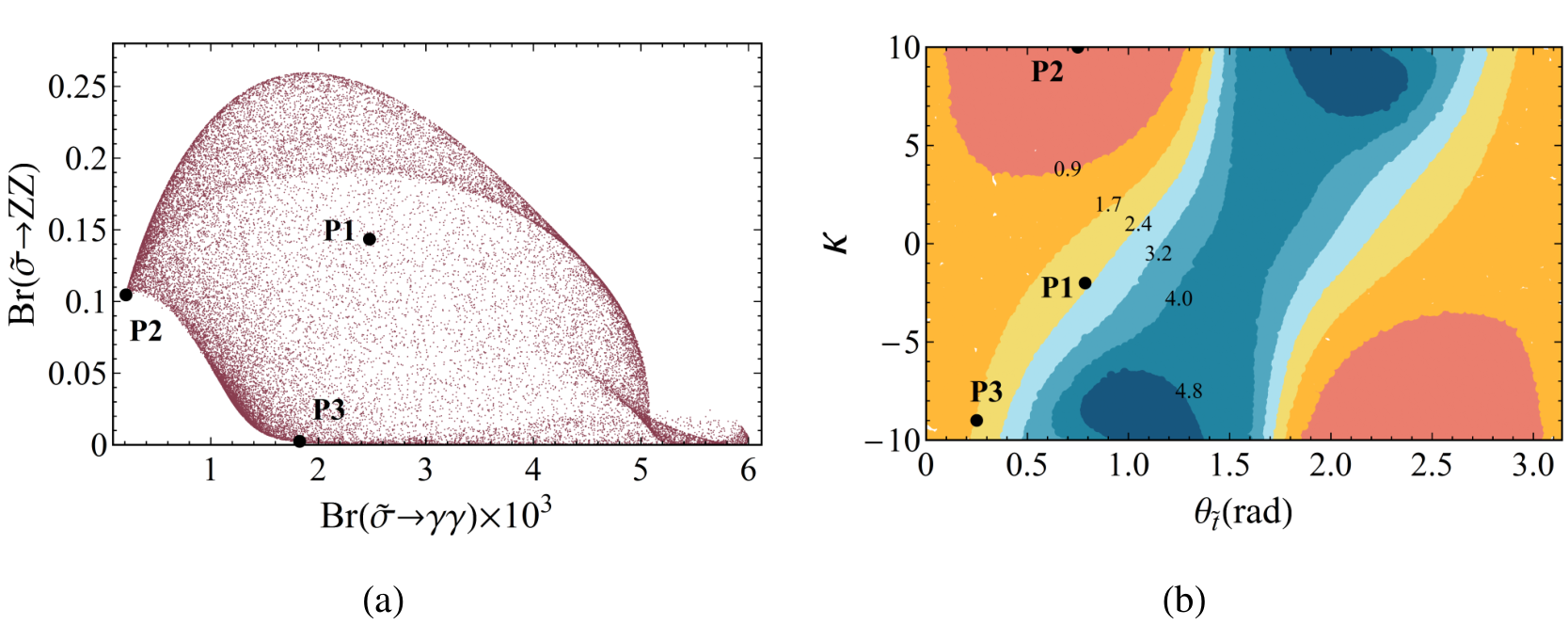
Now we study the dependence on the MSSM parameters for the resonant cross section. Since the resonant cross section is proportional to the branching ratio for the decay channel, it suffices to examine the MSSM parameter dependence of the stoponium branching ratios. We show the scatter plot for branching ratios for and in figure 7(a) with by randomly generating the four relevant MSSM parameters within the ranges:
| (61) |
Note that even though the decay rate for does not depend on the MSSM parameters, varies significantly within the range since the total decay rate changes according to the MSSM parameters. Our point in the parameter space P1 has sizable branching ratios for both channels. Below we will also consider two more pessimistic scenarios, P2 and P3. The point P2 corresponds to a scenario in which gets its minimal value. In this case there is a unique . The point P3 corresponds to close to its minimum, with the minimum possible subject to this constraint22 2 The branching ratios of and channel are , respectively for P1, , for P2, and , for P3.. These three benchmark points of the MSSM parameter set are shown in figure 7(a). Note that there is no point in the parameter space where both branching fractions are negligible. There is a curve, which is roughly a straight line, connecting points P2 and P3 that forms the boundary of the scatter plot. Moving along this curve one compensates for decreases in one branching ratio with increases in the other. It is clear that points along this curve correspond to worst-case scenarios for searching for stoponium in these channels: if we can exclude the existence of stoponium for parameter sets along this curve, than this will certainly be true for the remaining MSSM parameter space. We summarize explicit parameter choices for each benchmark point:
| (62) |
It turns out that each branching ratio is strongly dependent on and while the effects of and are minor. For illustration, we show contour plot of with respect to and in figure 7(b).
We now try to estimate the required luminosity to discover the stoponium resonance at current and future LHC runs. The required luminosity is evaluated by demanding significance for the signal events. We use the following formula for the significance [64]
| (63) |
where and represent the number of signal and background events. It is known that this formula is more reliable compared to the commonly used when the number of background events is small. If , Eq. (63) reduces to .
We take into account the reconstruction efficiency for photons, , in generating signal and background events for the channel. We set as given in Ref. [53]. For the channel, we consider the final states for reconstructing . We multiply the calculated cross section for by the branching fractions for decaying to leptons and the four lepton selection efficiency of as given in Ref. [65]. The generated SM background in the four lepton channels includes the virtual photon contribution. We expect that including channels will provide better statistics for the signal yield especially in the high mass region as discussed in Ref. [66].
We consider five different stoponium masses ranging between 400 and using the MSSM parameter values of the three benchmark points for both 8 and . This analysis will help determine the better search channel for the stoponium resonance signal for a given point in MSSM parameter space and for a given integrated luminosity. The results are shown in Tables 1 and 2.
| 400 GeV | 500 GeV | 600 GeV | 700 GeV | 800 GeV | ||
|---|---|---|---|---|---|---|
| P1 | 0.62 (171) | 0.13 (1197) | 0.032 (9654) | 0.008 () | 0.002 () | |
| P2 | 0.018 () | 0.011 () | 0.006 () | 0.002 () | 0.001 () | |
| P3 | 0.55 (212) | 0.097 (2186) | 0.020 () | 0.004 () | 0.001 () | |
| 2.1 | 0.70 | 0.34 | 0.14 | 0.06 | ||
| P1 | 0.085 (519) | 0.034 (1288) | 0.015 (3268) | 0.006 (8171) | 0.003 () | |
| P2 | 0.032 (3016) | 0.025 (2232) | 0.016 (2801) | 0.008 (5268) | 0.004 () | |
| P3 | 0.002 () | () | () | () | () | |
| 0.067 | 0.027 | 0.013 | 0.006 | 0.003 |
| 400 GeV | 500 GeV | 600 GeV | 700 GeV | 800 GeV | ||
|---|---|---|---|---|---|---|
| P1 | 2.3 (28) | 0.55 (173) | 0.15 (956) | 0.043 (6650) | 0.014 () | |
| P2 | 0.067 () | 0.047 () | 0.026 () | 0.012 () | 0.005 () | |
| P3 | 2.0 (34) | 0.40 (312) | 0.088 (2534) | 0.022 () | 0.006 () | |
| 4.4 | 1.7 | 0.67 | 0.41 | 0.21 | ||
| P1 | 0.31 (104) | 0.14 (223) | 0.066 (489) | 0.032 (1076) | 0.017 (2261) | |
| P2 | 0.12 (572) | 0.10 (378) | 0.073 (422) | 0.041 (707) | 0.022 (1413) | |
| P3 | 0.007 () | 0.002 () | () | () | () | |
| 0.16 | 0.070 | 0.035 | 0.019 | 0.010 |
For the run, the required luminosity rapidly grows as the stoponium mass increases in any of the parameter sets. It easily goes beyond the current and future LHC reach. We see that it is hopeless to observe the resonance signal for stoponium masses between 400 and in any of the benchmark parameter sets with the current accumulated LHC luminosity, .
On the other hand, for the run, we are able to explore the stoponium mass up to 500 in the first round of a future LHC run with of accumulated data. As we expect, for the parameter sets P1 and P2, the channel is the most promising for discovering stoponium, while in the case of P3 the channel is better than the channel. In order, for example, to see a 500 stoponium resonance signal we need at least 378 using both and channels regardless of the MSSM parameter sets. For a heavier stoponium mass, one needs the high-luminosity LHC run with upgraded instantaneous luminosity. We note if the expected stoponium resonance signal is not observed in the and/or channels we can exclude some of the MSSM parameter space in the - plane.
VI Conclusion
In this work we have studied the production of stoponium in collisions at the LHC. Our analysis focused on the MSSM scenario with light stops in the - GeV mass range, which are able to evade existing searches that look for stops that decay to neutralinos and top quarks. We used effective field theory to obtain a factorized form of the cross section. This allowed us to resum large threshold logarithms using RG equation methods up to NNLL accuracy. We verified explicitly that when NLO+NNLL results are considered, theoretical uncertainties are considerably reduced which highly improves the phenomenological predictions for the LHC. We included the enhanced Coulomb interactions responsible for creating the bound state of stops, stoponium, by including the NLO strong Coulomb Green‘s function. We provided formulas for both total and differential cross sections.
On the phenomenological side, we considered the decays of stoponium to and as promising channels for searching for the stoponium resonance in the mass range 400 to . After investigating MSSM parameter dependence, we found that and channels sensitively depend on and while the effects of other MSSM parameters are negligible. Therefore, one can impose constraints on and if the stoponium resonance signal is not observed. Our results indicated that one cannot exclude any mass value in this mass range with the currently accumulated LHC data at . On the other hand, for the first round of future LHC runs at with integrated luminosity, it should be possible to find stoponium if its mass is less than via either the or channels. We stress that this result does not depend on any particular choice of MSSM parameters. In this regard, searching in and for the stoponium resonance will serve as a complementary method for probing light stop scenarios in future LHC runs.
Acknowledgements.
We would like to thank Stephen Martin for pointing out some subtle issues regarding the phenomenological part of our work. C. Kim was supported by the Basic Science Research Program through NRF funded by MSIP (Grant No. 2012R1A1A1003015). C. Kim thanks KIAS for its hospitality during a visit to complete this work. A. Idilbi is supported by the U.S Department of Energy under Grant No. DE-SC0008745. T. Mehen is supported in part by the U.S. Department of Energy, Office of Nuclear Physics, under Contract No. DE-FG02-05ER41368. T. Mehen thanks ECT* for its hospitality during which part of this work was performed. Y.W. Yoon thanks the KIAS Center for Advanced Computation for providing computing resources. Y.W. Yoon thanks the L/EFT theory group of Duke University for its hospitality during a visit where part of this work was done.Appendix A Stoponium decay rate
Here we present the relevant formulas of stoponium decay rates at LO in . As we mentioned in Sec. V, we neglect contributions from another heavier stop, gluino and a heavy Higgs by assuming that they are much heavier than a light stop. The stoponium decay rate can be related with the cross section of stop pair annihilation through , where is the relative velocity between stops and is a stop bound state wave function at the origin. Then the decay rate has following conventional form
| (64) |
where the triangle function is given as .
In the small velocity limit, the matrix elements squared of each decay channel are
| (65) | |||||
| (66) | |||||
| (67) | |||||
| (68) | |||||
| (69) | |||||
| (70) | |||||
| (71) | |||||
| (72) |
Here, is the electric charge of the stop. The MSSM coupling constants are defined as
| (73) | |||||
| (74) | |||||
| (75) | |||||
| (76) | |||||
| (77) | |||||
| (78) | |||||
| (79) | |||||
| (80) | |||||
| (81) | |||||
| (82) | |||||
| (83) |
where are the sine and cosine of the weak mixing angle, and and are the sine and cosine of stop mixing angle . is the Higgs VEV, fixed by . We refer to Ref. [67] to obtain the Feynman rules for the MSSM.
Appendix B Anomalous dimensions
In this section we summarize all the formulas for the anomalous dimensions that are necessary to perform resummation up to NNLL. First of all, the function is expanded in as
| (84) |
where we have
| (85) |
The convention for the expansion of anomalous dimension in is
| (86) |
The anomalous dimension for hard scattering of Higgs boson production is equivalent to that of stoponium production since the effective theory calculations are the same at the hard matching scale (whether it is the mass of the Higgs boson or the stop pair). The coefficients of are [68, 69]
| (87) |
up to two-loop order. The anomalous dimension for the soft function is obtained with the aid of the relation: , where is the coefficient of the term in the Altarelli-Parisi splitting function which reads [70]
| (88) |
The solution for the Sudakov exponent is expressed as [62]
| (89) | |||||
where . The coefficients of the expansion (in ) of the cusp anomalous dimension for the Wilson loop in the adjoint representation (up to third order in ) read [71, 72]
| (90) | |||||
The solution for the exponent is expressed as
| (91) | |||||
The exponent can also be expressed in a similar way.
Appendix C Coulomb Green’s Function
In this section, we present the formula of the Greens’s function up to NLO in that is used in phenomenological analysis of this work. Especially, we explicitly show the analytic continuation of the Green’s function at NLO which is essential for numerical implementation of it when the bound state resonance is narrow.
The Green’s function of the Schrödinger equation with Coulomb potential up to NLO between heavy colored particles was calculated in Ref. [73]. We refer to Refs. [74, 75] for the explicit formula of the Greens’s function at the origin for the color-singlet stoponium bound state which is described by
| (92) |
The LO and NLO Green’s functions and read
| (93) | |||||
| (94) | |||||
where . and are defined by
| (95) |
The functions are defined by
| (96) |
The appropriate Coulomb scale is estimated by .
It is nontrivial to evaluate the hypergeometric function in the NLO Green’s function. The series expansion of the hypergeometric function with unit argument is convergent if
| (97) |
Therefore, the hypergeometric function is well defined in . Since we encounter above the resonance peak, we need to analytically continuate the hypergeometric function into the complex plane in which .
In general, the hypergeometric function with unit argument can be analytically continuated by using the relation [76]
| (98) |
We note that the value of Eq. (97) in the right-hand side is increased by 1. Thus, by repeatedly applying this relation one can represent any hypergeometric function with unit argument in terms of convergent hypergeometric functions.
On the other hand, the method described in Ref. [75] is useful for investigating the asymptotic behavior of the Green’s function near rhe resonance region. The explicit expansion of is given by
| (99) |
This infinite sum can be handled by Ref. [77] and be represented in terms of harmonic sums [78, 79],
| (100) |
The harmonic sums are related with functions as follows
| (101) | |||||
| (102) |
The nested harmonic sum can be represented in integral form [80],
| (103) |
This integral form is well defined for . The analytic continuation into is straightforward:
| (104) | |||||
where positive integer is chosen such that . In all, we finally obtain an expression of an analytically continuated NLO Green’s function which can be evaluated in any complex value of :
| (105) | |||||
We note that the resonance peaks arise when becomes positive integer values, that is for narrow resonance states. We use this formula for the Green’s function at NLO throughout the numerical analysis of this work.
References
- [1] S. Dimopoulos and G. F. Giudice, Phys. Lett. B 357, 573 (1995) [hep-ph/9507282].
- [2] A. Pomarol and D. Tommasini, Nucl. Phys. B 466, 3 (1996) [hep-ph/9507462].
- [3] A. G. Cohen, D. B. Kaplan and A. E. Nelson, Phys. Lett. B 388, 588 (1996) [hep-ph/9607394].
- [4] R. Kitano and Y. Nomura, Phys. Rev. D 73, 095004 (2006) [hep-ph/0602096].
- [5] Y. Kats, P. Meade, M. Reece and D. Shih, JHEP 1202, 115 (2012) [arXiv:1110.6444 [hep-ph]].
- [6] C. Brust, A. Katz, S. Lawrence and R. Sundrum, JHEP 1203, 103 (2012) [arXiv:1110.6670 [hep-ph]].
- [7] C. Brust, A. Katz and R. Sundrum, JHEP 1208, 059 (2012) [arXiv:1206.2353 [hep-ph]].
- [8] M. Papucci, J. T. Ruderman and A. Weiler, JHEP 1209, 035 (2012) [arXiv:1110.6926 [hep-ph]].
- [9] J. R. Espinosa, C. Grojean, V. Sanz and M. Trott, JHEP 1212, 077 (2012) [arXiv:1207.7355 [hep-ph]].
- [10] C. Boehm, A. Djouadi and M. Drees, Phys. Rev. D 62, 035012 (2000) [hep-ph/9911496].
- [11] P. Huet and A. E. Nelson, Phys. Rev. D 53, 4578 (1996) [hep-ph/9506477].
- [12] M. Carena, G. Nardini, M. Quiros and C. E. M. Wagner, Nucl. Phys. B 812, 243 (2009) [arXiv:0809.3760 [hep-ph]].
- [13] Y. Li, S. Profumo and M. Ramsey-Musolf, Phys. Lett. B 673, 95 (2009) [arXiv:0811.1987 [hep-ph]].
- [14] A. Delgado, G. F. Giudice, G. Isidori, M. Pierini and A. Strumia, Eur. Phys. J. C 73, 2370 (2013) [arXiv:1212.6847 [hep-ph]].
- [15] J. Cao, C. Han, L. Wu, J. M. Yang and Y. Zhang, JHEP 1211, 039 (2012) [arXiv:1206.3865 [hep-ph]].
- [16] G. D. Kribs, A. Martin and A. Menon, Phys. Rev. D 88, 035025 (2013) [arXiv:1305.1313 [hep-ph]].
- [17] K. Kowalska and E. M. Sessolo, Phys. Rev. D 88, 075001 (2013) [arXiv:1307.5790 [hep-ph]].
- [18] C. Han, K. -i. Hikasa, L. Wu, J. M. Yang and Y. Zhang, JHEP 1310, 216 (2013) [arXiv:1308.5307 [hep-ph]].
- [19] C. Kim and T. Mehen, Phys. Rev. D 79, 035011 (2009) [arXiv:0812.0307 [hep-ph]].
- [20] A. Idilbi, C. Kim and T. Mehen, Phys. Rev. D 82, 075017 (2010) [arXiv:1007.0865 [hep-ph]].
- [21] M. Drees and M. M. Nojiri, Phys. Rev. D 49, 4595 (1994) [hep-ph/9312213].
- [22] S. P. Martin, Phys. Rev. D 77, 075002 (2008) [arXiv:0801.0237 [hep-ph]].
- [23] C. W. Bauer, S. Fleming and M. E. Luke, Phys. Rev. D 63, 014006 (2000) [arXiv:hep-ph/0005275]; C. W. Bauer, S. Fleming, D. Pirjol and I. W. Stewart, Phys. Rev. D 63 (2001) 114020 [arXiv:hep-ph/0011336].
- [24] C. W. Bauer, D. Pirjol and I. W. Stewart, Phys. Rev. D 65 (2002) 054022 [arXiv:hep-ph/0109045].
- [25] C. W. Bauer, D. Pirjol and I. W. Stewart, Phys. Rev. D 68, 034021 (2003) [hep-ph/0303156].
- [26] M. Beneke, P. Falgari and C. Schwinn, Nucl. Phys. B 842, 414 (2011) [arXiv:1007.5414 [hep-ph]].
- [27] P. Falgari, C. Schwinn and C. Wever, JHEP 1206, 052 (2012) [arXiv:1202.2260 [hep-ph]].
- [28] M. Beneke, P. Falgari, J. Piclum, C. Schwinn and C. Wever, arXiv:1312.0837 [hep-ph].
- [29] U. Langenfeld and S. -O. Moch, Phys. Lett. B 675, 210 (2009) [arXiv:0901.0802 [hep-ph]].
- [30] U. Langenfeld, JHEP 1107, 052 (2011) [arXiv:1011.3341 [hep-ph]].
- [31] U. Langenfeld, S. -O. Moch and T. Pfoh, JHEP 1211, 070 (2012) [arXiv:1208.4281 [hep-ph]].
- [32] T. Pfoh, JHEP 1305, 044 (2013) [arXiv:1302.7202 [hep-ph]].
- [33] W. Beenakker, S. Brensing, M. Kramer, A. Kulesza, E. Laenen and I. Niessen, JHEP 1008, 098 (2010) [arXiv:1006.4771 [hep-ph]].
- [34] W. Beenakker, S. Brensing, M. Kramer, A. Kulesza, E. Laenen and I. Niessen, JHEP 1201, 076 (2012) [arXiv:1110.2446 [hep-ph]].
- [35] W. Beenakker, T. Janssen, S. Lepoeter, M. Kramer, A. Kulesza, E. Laenen, I. Niessen and S. Thewes et al., JHEP 1310, 120 (2013) [arXiv:1304.6354 [hep-ph]].
- [36] A. Broggio, A. Ferroglia, M. Neubert, L. Vernazza and L. L. Yang, JHEP 1307, 042 (2013) [arXiv:1304.2411 [hep-ph]].
- [37] A. Broggio, A. Ferroglia, M. Neubert, L. Vernazza and L. L. Yang, arXiv:1312.4540 [hep-ph].
- [38] G. Aad et al. [ATLAS Collaboration], Phys. Rev. Lett. 109, 211802 (2012) [arXiv:1208.1447 [hep-ex]]. Phys. Rev. Lett. 109, 211803 (2012) [arXiv:1208.2590 [hep-ex]]. JHEP 1211, 094 (2012) [arXiv:1209.4186 [hep-ex]]. Eur. Phys. J. C 72, 2237 (2012) [arXiv:1208.4305 [hep-ex]]. https://twiki.cern.ch/twiki/bin/view/AtlasPublic, Summary plot for direct stop pair production
- [39] S. Chatrchyan et al. [CMS Collaboration], Eur. Phys. J. C 73, 2677 (2013) [arXiv:1308.1586 [hep-ex]].
- [40] M. Beneke, P. Falgari and C. Schwinn, Nucl. Phys. B 828, 69 (2010) [arXiv:0907.1443 [hep-ph]].
- [41] K. -i. Hikasa and M. Kobayashi, Phys. Rev. D 36, 724 (1987).
- [42] W. Porod and T. Wohrmann, Phys. Rev. D 55, 2907 (1997) [Erratum-ibid. D 67, 059902 (2003)] [hep-ph/9608472].
- [43] P. Falgari, C. Schwinn and C. Wever, JHEP 1301, 085 (2013) [arXiv:1211.3408 [hep-ph]].
- [44] J. Chay and C. Kim, Phys. Rev. Lett. 110, 122002 (2013) [arXiv:1212.4257 [hep-ph]].
- [45] J. Chay and C. Kim, JHEP 1309, 126 (2013) [arXiv:1303.1637 [hep-ph]].
- [46] S. Fleming, A. K. Leibovich and T. Mehen, Phys. Rev. D 74, 114004 (2006) [hep-ph/0607121].
- [47] J. E. Younkin and S. P. Martin, Phys. Rev. D 81, 055006 (2010) [arXiv:0912.4813 [hep-ph]].
- [48] T. Becher and M. Neubert, Phys. Rev. Lett. 97, 082001 (2006) [hep-ph/0605050].
- [49] T. Becher, M. Neubert and B. D. Pecjak, JHEP 0701, 076 (2007) [hep-ph/0607228].
- [50] S. Chatrchyan et al. [CMS Collaboration], Phys. Lett. B 723, 280 (2013) [arXiv:1212.1910 [hep-ex]].
- [51] CMS Collaboration [CMS Collaboration], CMS-PAS-EXO-12-024.
- [52] V. Barger, M. Ishida and W. .-Y. Keung, Phys. Rev. Lett. 108, 081804 (2012) [arXiv:1110.2147 [hep-ph]].
- [53] G. Aad et al. [ATLAS Collaboration], Phys. Lett. B 716, 1 (2012) [arXiv:1207.7214 [hep-ex]].
- [54] S. Chatrchyan et al. [CMS Collaboration], Phys. Lett. B 716, 30 (2012) [arXiv:1207.7235 [hep-ex]].
- [55] A. D. Martin, W. J. Stirling, R. S. Thorne and G. Watt, Eur. Phys. J. C 63, 189 (2009) [arXiv:0901.0002 [hep-ph]].
- [56] H. L. Lai et al. [CTEQ Collaboration], Eur. Phys. J. C 12, 375 (2000) [hep-ph/9903282].
- [57] W. Beenakker, M. Kramer, T. Plehn, M. Spira and P. M. Zerwas, Nucl. Phys. B 515, 3 (1998) [hep-ph/9710451].
- [58] G.Aad at al. (ATLAS Collaboration), JINST 3, S08003 (2008)
- [59] J. M. Campbell, R. K. Ellis and C. Williams, JHEP 1107, 018 (2011) [arXiv:1105.0020 [hep-ph]].
- [60] The ATLAS Collaboration, ATLAS-CONF-2012-090 (2012)
- [61] The ATLAS Collaboration, ATLAS-CONF-2012-091 (2012)
- [62] T. Becher, M. Neubert and G. Xu, JHEP 0807, 030 (2008) [arXiv:0710.0680 [hep-ph]].
- [63] V. Ahrens, T. Becher, M. Neubert and L. L. Yang, Eur. Phys. J. C 62, 333 (2009) [arXiv:0809.4283 [hep-ph]].
- [64] G. Cowan, K. Cranmer, E. Gross and O. Vitells, Eur. Phys. J. C 71, 1554 (2011) [arXiv:1007.1727 [physics.data-an]].
- [65] G. Aad et al. [ATLAS Collaboration], Phys. Lett. B 712, 331 (2012) [arXiv:1203.0718 [hep-ex]].
- [66] T. Aaltonen et al. [CDF Collaboration], Phys. Rev. D 85, 012008 (2012) [arXiv:1111.3432 [hep-ex]].
- [67] J. Rosiek, hep-ph/9511250.
- [68] A. Idilbi, X. -d. Ji, J. -P. Ma and F. Yuan, Phys. Rev. D 73, 077501 (2006) [hep-ph/0509294].
- [69] A. Idilbi, X. -d. Ji and F. Yuan, Phys. Lett. B 625, 253 (2005) [hep-ph/0507196].
- [70] A. Vogt, S. Moch and J. A. M. Vermaseren, Nucl. Phys. B 691, 129 (2004) [hep-ph/0404111].
- [71] I. A. Korchemskaya and G. P. Korchemsky, Phys. Lett. B 287, 169 (1992).
- [72] S. Moch, J. A. M. Vermaseren and A. Vogt, Nucl. Phys. B 688, 101 (2004) [hep-ph/0403192].
- [73] M. Beneke, A. Signer and V. A. Smirnov, Phys. Lett. B 454, 137 (1999) [hep-ph/9903260].
- [74] Y. Kiyo, J. H. Kuhn, S. Moch, M. Steinhauser and P. Uwer, Eur. Phys. J. C 60, 375 (2009) [arXiv:0812.0919 [hep-ph]].
- [75] M. Beneke, P. Falgari, S. Klein and C. Schwinn, Nucl. Phys. B 855, 695 (2012) [arXiv:1109.1536 [hep-ph]].
- [76] T. Huber and D. Maitre, Comput. Phys. Commun. 175, 122 (2006) [hep-ph/0507094].
- [77] I. Bierenbaum, J. Blumlein, S. Klein and C. Schneider, Nucl. Phys. B 803, 1 (2008) [arXiv:0803.0273 [hep-ph]].
- [78] J. A. M. Vermaseren, Int. J. Mod. Phys. A 14, 2037 (1999) [hep-ph/9806280].
- [79] J. Blumlein and S. Kurth, Phys. Rev. D 60, 014018 (1999) [hep-ph/9810241].
- [80] J. Blumlein, Comput. Phys. Commun. 180, 2218 (2009) [arXiv:0901.3106 [hep-ph]].