Particle current fluctuations in a variant of asymmetric Glauber model
Abstract
We study the total particle current fluctuations in a one-dimensional stochastic system of classical particles consisting of branching and death processes which is a variant of asymmetric zero-temperature Glauber dynamics. The full spectrum of a modified Hamiltonian, whose minimum eigenvalue generates the large deviation function for the total particle current fluctuations through a Legendre-Fenchel transformation, is obtained analytically. Three examples are presented and numerically exact results are compared to our analytical calculations.
Keywords:
driven-diffusive systems in one-dimension, particle current fluctuations,Glauber modelpacs
05.40.-a,05.70.Ln,05.20.-yI Introduction
Most of one-dimensional non-equilibrium systems with stochastic dynamics show unique collective behaviors in their steady-states which usually can not be found in their equilibrium counterparts. Non-equilibrium phase transition and shock formation are two examples of these remarkable behaviors. Non-equilibrium systems are also interesting to study from a mathematical point of view. These systems have opened up new horizon of research in the field of exactly solvable systems [1, 2].
During the last decade several non-equilibrium exactly solvable systems have been introduced and studied in related literature. On the other hand, different mathematical techniques have been developed to study their steady-state properties. A matrix method, known as the matrix product method, is introduced and used to calculate the steady-state and the average value of the physical quantities in the steady-state of these systems [3]. The excitations, which give the relaxation times, can also be obtained using the Bethe Ansatz [4]. Recently, there has been attempts to establish connections between Bethe Ansatz and matrix product method [5]. Other interesting quantities include the large deviation function for the probability distribution of fluctuating quantities, such as the particle current, in the steady-state of these systems [6, 7]. The large deviation function can be obtained, through a Legendre-Fenchel transformation, from the minimum eigenvalue of a modified Hamiltonian. We are then basically left with finding the minimum eigenvalue of a matrix. The number of systems for which this quantity can be calculated exactly is very limited.
In this paper we consider a stochastic system of classical particles in which the particles interact with each other according to a variant of the zero-temperature Glauber dynamics on a lattice with open boundaries [11, 12, 13]. More precisely the particles are injected and extracted from the first and the last sites of the lattice respectively. In the bulk of the lattice, on the other hand, the particles are subjected to totally asymmetric branching and death processes. The steady-state of this system has already been calculated using the matrix product method [14]. It is known that this steady-state can be written as a linear combination of product shock measures with one shock front and that these shock fronts have simple random walk dynamics [15].
We are specially interested in the total particle current fluctuations in this system. As we mentioned, the large deviation function for the particle current fluctuations can be obtained from the Legendre-Fenchel transformation of the minimum eigenvalue of a modified Hamiltonian. This modified Hamiltonian can be constructed from the stochastic time evolution operator of the system (sometimes called the Hamiltonian). This can be done by multiplying the non-diagonal elements of the Hamiltonian of the system by an exponential factor which counts the particle jumps contributing to the total particle current, see for example [8, 9, 10]. It turns out that the modified Hamiltonian associated with the total particle current fluctuations can be fully diagonalized. The key point is to change the basis of the vector space in an appropriate way by introducing a product shock measure with multiple shock fronts. In this new basis the modified Hamiltonian becomes an upper block-bidiagonal matrix which is much easier to work with, because we only need to diagonalize the diagonal blocks.
Our analytical investigations reveal that for the small particle current fluctuations (smaller than the average particle current in the steady-state to be more precise) the eigenvector associated with the minimum eigenvalue of the modified Hamiltonian should be written as a linear combination of product shock measures with a single shock front. In contrast, for the large particle current fluctuations (larger than the average particle current in the steady-state to be more precise) it should be written as a linear combination of product shock measures with more than one shock front. The validity of our analytical calculations is checked by comparing the analytical results with those obtained from numerical diagonalization of the modified Hamiltonian.
This paper is organized as follows. In the second section we will review the known results on the steady-state properties of the system. The total particle current is also introduced and its average value in the steady-state is calculated. In the third section we will briefly review the basics of the particle current fluctuations. The forth section is devoted to the diagonalization of the modified Hamiltonian. The minimum eigenvalue of the modified Hamiltonian will be discussed in the fifth section. We will compare the analytical and numerical results in the sixth section. The concluding remarks are also given in the last section.
II Steady-State
Let’s consider a lattice of length . We assume that each lattice site can be occupied by at most one particle or a vacancy. The reaction rules between two consecutive sites and on the lattice are as follow
| (1) |
in which a particle (vacancy) is labeled with (). A particle can enter the system from the left boundary of the lattice with the rate . A particle can also leave the system from the right boundary with the rate . This model is an asymmetric variant of zero-temperature Glauber dynamics [11, 12, 13]. The time evolution of the probability distribution vector is given by a master equation [2]
| (2) |
where the Hamiltonian is an stochastic square matrix
| (3) |
in which is a identity matrix and that we have defined
Introducing the basis kets
the matrix representation of in the basis of and that of and in the basis of are given by
The right eigenvector with vanishing eigenvalue of Hamiltonian gives the steady-state probability distribution vector of the system. It is known that this vector can be written as a linear combination of product shock measures with a single shock front [15]. It turns out that the dynamics of the position of a shock front is similar to that of a biased random walker moving on a finite lattice with reflecting boundaries. This steady-state probability distribution vector has also been obtained using a matrix product method in [14]. By associating the operators and to the presence of a vacancy and a particle in a given lattice site, the steady-state weight of any configuration is proportional to
| (4) |
in which if the lattice-site is empty and if it is occupied by a particle. In (4), and are two auxiliary vectors. It has been shown that these two operators and vectors have a two-dimensional matrix representation given by [14]
| (5) |
in which is a free parameter. Using (4) and (5) one can easily calculate the weight of any configuration in the steady-state and also the average value of the physical quantities, such as the particle current, in the long-time limit.
Let us call the average local density of particles at the lattice site at time . Using (1) and considering the injection and extraction of particles at the boundaries the time evolution of this quantity is given by
| (6) | |||||
in which . The average local density of particles is related to the average particle current through a continuity equation
| (7) |
for . We define as the average local particle current from the lattice site to at time . is also called a source term. In (7) we have also assumed that . In the steady-state the time dependency of the quantities will be dropped and we find
| (8) |
Comparing (6) and (7) one finds the following relation for the average particle current in the steady-state
| (9) |
and also the source terms which are defined as follows
| (10) | |||||
in which . The average particle current in (9) can be understood by investigating (1). The second dynamical rule in (1) clearly increase the particle current. The first dynamical rule in (1) can be considered as a backward movement of a vacancy. This is equivalent to a forward movement of a particle which, again, increases the particle current. Similar examples of particle current in the presence of source terms can be found in [16].
The average local particle current in the steady-state can be calculated using the matrix product method. The result is
in which we have defined . Defining the total particle current as
| (11) |
it is easy to see that in the limit of we have
| (12) |
This indicates that the system undergoes a phase transition at . The phase () is called the low-density (high-density) phase.

III Particle Current Fluctuations
Assuming that the large deviation principle holds, the probability distribution for observing the total particle current in the system is given by
| (13) |
which is valid for . The large deviation function measures the rate at which the total particle current deviates from its average value. It is known that the large deviation function is, according to the Gärtner-Ellis theorem, the Legendre-Fenchel transform of the minimum eigenvalue of a modified Hamiltonian , denoted by , [6]
| (14) |
The modified Hamiltonian is defined as follows
| (15) |
in which
Note that since the modified Hamiltonian defined in (15) becomes equal to the stochastic time evolution operator given in (3) at then we have . Finally, the first derivative of the minimum eigenvalue respect to at gives the total current defined in (11)
| (16) |
In the following section we will show that , defined in (15), can be diagonalized exactly.
IV Diagonalization of
In order to diagonalize the modified Hamiltonian defined in (15) we start with redefining the basis of the vector space by introducing the following product shock measure with shock fronts
| (17) |
in which for an even and for an odd and that . A simple sketch of such a product shock measure with multiple shock fronts is given in Fig. 1.
For a given the number of these vectors is simply given by a Binomial coefficient . Now the dimensionality of the vector space constructed with these vectors can be obtained as
| (18) |
regardless of whether is even or odd. The vectors (17) make a complete orthonormal basis for our -dimensional vector space. Assuming is an even number 11 1 Our approach is not affected when the system size is an odd number. One should only consider everywhere throughout this section., in the basis
| (19) |
the modified Hamiltonian (15) has the following upper block-bidiagonal matrix representation
| (20) |
in which for is a matrix and for is a matrix. The matrix elements of these matrices are given explicitly in the Appendix A.
Although the modified Hamiltonian (20) is not a stochastic matrix; however, its matrix structure suggests the following picture which will be discussed in more detail in the forthcoming sections. Acting (20) on with , which is a product shock measure with a single shock front, gives a linear combination of product shock measures with a single shock front. These series of evolution equations are quite similar to the evolution equations for a particle at the lattice site performing a biased random walk on a one-dimensional lattice with reflecting boundaries. In other words, the vectors define an invariant sector, which will be called , in the sense that acting on any member of this sector gives a linear combination of the vectors in the same sector. The matrix elements of in (20) determine the coefficients of these linear expansions.
On the other hand, acting (20) on with , which is a product shock measure with three shock fronts, gives a linear combination of the product shock measures with a single or three shock fronts. These series of evolution equations are quite similar to those of two random walkers at the lattice sites and besides an obstacle at the lattice site which does not have any dynamics. The reason that the shock front at the lattice site (or the obstacle) does not have any dynamics can be easily understood by looking at (1). In fact, the position of a shock front of type is not affected by these dynamical rules. As long as the random walkers are more than a single lattice site away from the obstacle, they perform biased random walks on the lattice. The random walkers also reflect from the boundaries of the lattice whenever they reach to the boundaries. When one of the random walkers arrives at an obstacle, the random walker and the obstacle both disappear; however, the other random walker continues to perform a biased random walk on the lattice. No new random walker or obstacle will be created once they disappear. The matrices and are responsible for the dynamics of these random walkers. The above argument suggests that the vectors in besides the vectors define an invariant sector, which will be called . Acting on any member of this sector gives a linear combination of the vectors in the same sector.
The next invariant sector, which will be called , is defined by the vectors in and in which . In this case we have three random walkers which are separated from each other by two obstacles. Once a random walker meets an obstacle at two consecutive lattice sites, they disappear. The matrices and generates the dynamics of the random walkers and their interactions with the obstacles.
This procedure can be continued to see that there are invariant sectors.
In order to find the eigenvalues of the modified Hamiltonian (20) we can follow two equivalent scenarios. From one hand, the eigenvectors of this matrix can be written as a linear combination of the vectors in each invariant sector. This helps us find all of its eigenvalues. On the other hand, since the eigenvalues of the modified Hamiltonian are equal to those of ’s for , one can diagonalize each separately to calculate the eigenvalues of (20). We will employ the second approach which is the subject of the forthcoming sections.
IV.1 Diagonalization of
is a tridiagonal matrix which has, in the basis (17), the following matrix representation
The structure of this matrix reminds us of the evolution operator for a biased random walk moving on a one-dimensional lattice of length with reflecting boundaries –although the reader should note that the evolution operator is not a stochastic matrix. In an appropriate basis the evolution equations for the position of the random walker can be formally written as follows
with . Now the eigenvectors and also the eigenvalues of can be obtained using the same approach employed in [17] by writing
| (21) |
and considering
| (22) |
Substituting (22) in (21) and using the evolution equations for the shock front one can calculate ’s by applying a plane wave Ansatz. Defining
and
we find
| (23) |
in which
It also turns out that the eigenvalues of are given by
| (24) |
The equation governing is also given by
| (25) |
It can be seen that the equation (25) has solutions. Two of these solutions i.e. have to be excluded since for these values of the corresponding eigenvector vanishes. On the other hand, if is solution for (25) then is also a solution. This means that the remaining solutions result in eigenvalues. For the pair corresponds to the eigenvalue . Finally, it can be shown that the solutions of the equation (25) are either phases i.e. or they are real numbers. For the phase solutions and the smallest eigenvalue in this case is given by
| (26) |
The real solutions of the equation (25) are much easier to be found in the thermodynamic limit . Let us restrict the real solutions to . It turns out that the equation (25) has two real solutions in the thermodynamic limit
| (27) |
where is defined as follows
Substituting (27) in (24) gives the corresponding eigenvalues which will be denoted by and . Whenever these eigenvalues exist, they will be definitely smaller than . The conditions under which and exist, will be discussed later.
IV.2 Diagonalization of
In the basis (17) the matrix is a block diagonal matrix with blocks. These blocks will be called with . On the other hand, for a given , is a -dimensional block tridiagonal matrix with the following structure
in which and are square matrices whose matrix representations are given in Appendix B. On the other hand, we have defined , and where is a identity matrix. Noting that
it is easy to check the dimensionality of .
Investigating the structure of for a given suggests that it can be regarded as a non-stochastic evolution operator for two biased random walkers, moving on a one-dimensional lattice of length with reflecting boundaries, which are separated by an obstacle. Let us denote the position of the first and the second random walker on the lattice by and respectively. The obstacle is at the lattice site . For a fixed the random walkers can only hop into the lattice sites which satisfy the condition . In terms of the matrix elements of , both random walkers reflect from the boundaries and also the obstacle. One should note that the matrix , in contrast to , does not allow the random walkers to merge with the obstacles. We remind the reader that ’s in (20) were responsible for disappearance of the random walkers and the obstacles.
For a given let us introduce an appropriate -dimensional basis with and . We arrange these vectors as . In this basis the evolution equations for the random walkers can be written as follows
| (28) | |||||
These equations can be used to find the eigenvalues and eigenvectors of . The reader can easily convince himself that in the above mentioned basis, the matrices ’s are responsible for moving the position of the second random walker while ’s are responsible for moving the position of the first random walker. For a given , the eigenvalue equation
| (29) |
can now be solved by using (28) and introducing
| (30) |
By considering a plane wave ansatz and after some straightforward calculations one finds that, for a given , the coefficients are given by
for and in which
The eigenvalues of are also given by
| (31) |
in which the equations governing and are
| (32) |
The first equation in (32) has solutions while the second equation has solutions. Excluding the solutions and and noting that if the pair is a solution then the pairs , and are also the solution, one finds solutions (or eigenvalues) by mixing the solutions of the equations (32).
IV.3 Diagonalization of
In the basis (17) the matrix is a block diagonal matrix. Our procedure in the preceding sections can be continued to see that each block of for can be regarded as a non-stochastic evolution operator for biased random walkers at the positions which are separated by obstacles at the positions given that . In other words, for the positions of the obstacles and the random walkers should satisfy the following constraints
| (33) |
with and . For a given each block of , which will be called , is a -dimensional square matrix where is given by
with the following property
In order to diagonalize we consider an appropriate -dimensional basis and write
in which the eigenvectors of are written as follows
| (34) |
The coefficients can be calculated using a plane wave ansatz and one finds
in which
The eigenvalues are also given by
| (35) |
in which ’s satisfy the following equations
| (36) |
In summary, the eigenvalues of can be calculated as follows: we first fix the position of the obstacles which should satisfy the first relation in (33). We will then solve the equations (36) and substitute their solutions in (35) which gives the corresponding eigenvalues. For each set of one find eigenvalues.
Now that all of the eigenvalues of the modified Hamiltonian (15) are known, we discuss about the smallest one in the forthcoming section from which the large deviation function for the total particle current can be calculated.

V Minimum eigenvalue of
It is clear that the minimum eigenvalue of the modified Hamiltonian depends on both the microscopic reaction rates and also . For each value of there are eigenvalues. This section is divided into two parts. In the first part we will consider the case . The second part is devoted in the case .
V.1 The case
The formula (35) suggests that as the minimum eigenvalue of should come from the eigenvalues of with the least number of random walkers, which is in this case i.e. the eigenvalues of . Let us work in the thermodynamic limit . In this limit, has two discrete eigenvalues and which can be calculated by substituting (27) in (24). These two eigenvalues go to zero as . We have found that for the minimum eigenvalue of the modified Hamiltonian is either or of depending on the values of the microscopic reaction rates and and also on . Defining
we bring a summery of the results in the following:
- •
In this phase, for , we have . For the minimum eigenvalue can be determined using the left panel of Fig. 2. As can be seen in the region III (the shaded area) the minimum eigenvalue is given by while it is given by in the regions I and II. The difference between these regions is related to the asymptotic behavior of the minimum eigenvalue when which is given by(37) - •
In this phase, for , we have . For the minimum eigenvalue can be determined using the right panel of Fig. 2. As can be seen in the region I (the shaded area) the minimum eigenvalue is given by while it is given by in the regions II and III. The asymptotic behaviors of the minimum eigenvalue in different regions is given by (37).
Using the above description of the minimum eigenvalue and (16) one can easily reproduce the results in (12).
It is worth mentioning here that the first derivative of the minimum eigenvalue is not continuous at . This means that the large deviation function for the total particle current fluctuations, which can be obtained using (14), is a linear function of for [6]
| (38) |
where for
and that for
The minimum eigenvalue of the modified Hamiltonian for generates, using (14), the large deviation function for the total particle current fluctuations for .
V.2 The case
For the situation is quite different. Let us first define as the smallest eigenvalue of . We have found that for a given finite the minimum eigenvalue of the modified Hamiltonian is given by for in which by defining and . Here is a discrete parameter which maximizes
| (39) |
and that it can take one of the following values
| (40) |

This means that in order to calculate the large deviation function for the total particle current in a system of length , we only need to know the minimum eigenvalues of ’s for . This has been shown schematically in Fig. 3. The inset of this figure shows as a function of . For instance, for a system of length we only need to know up to . This can be understood as follows. Let us assume that as the minimum eigenvalue of the modified Hamiltonian is given by which can be obtained from (35) by substituting . is the number of random walkers which can be obtained from (40). We are actually looking for the value of for which (35) is minimum. One can easily see that as the equations (36) become
in which ’s should satisfy (33). It turns out that these equations generate the minimum eigenvalue of (35) provided that the distribution of the obstacles on the lattice is uniform i.e.
which means with . It is now clear that for very small and negative values of , (35) takes its minimum value provided that the expression
becomes maximum.
We have not been able to find exact analytical expressions for ’s for ; however, it is possible to find numerically by solving the following equation
| (41) |
Our exact numerical calculations show that although the minimum eigenvalue of the modified Hamiltonian is continuous at ’s, its first derivative is not continuous at these points which results in
for where
We have also found that, for a given finite , decreases as increases. This will be discussed in the next section in terms of three examples.
In what follows we will consider the large- limit which seems to be much easier to manage. It turns out that for , for drops to zero as . On the other hand, it can be shown that in the thermodynamic limit we have
This means that in the large- limit, we only need to work with the minimum eigenvalues of and i.e.
At we have found that
| (42) |
which can be explained as follows. For , as approaches to from above, we find using (24) that
| (43) |
where is the real solution of (25) for which is given by and for and respectively. On the other hand, as approaches to from below we have
| (44) | |||||
in which ’s for are the solutions of the equations (36) at for . We have numerically checked that for the solutions of (36) satisfy
while for
Replacing these into (44) and comparing it with (43) confirms (42).
For and in the large- limit, is approximately given by
The minimum eigenvalue of the modified Hamiltonian for generates, using (14), the large deviation function for the total particle current fluctuations for .
In the next section we will check the validity of the above mentioned results by studying three different examples.
VI Examples: Numerical results
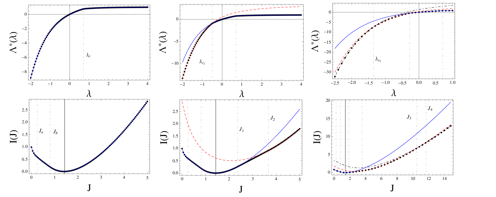
In what follows we will discuss three examples in detail. These examples consist of systems of length and . Assuming , , and , the results are given in Fig. 4 where we have plotted and its Legendre-Fenchel transformation obtained from two different approaches. The first approach is the direct diagonalization of given by (15) and the second approach is the use of (35) by solving the equations (36). Note that, according to (12), the average total particle current in this phase is .
As can be seen in the inset of Fig. 3, for a system of length , the minimum eigenvalue of the modified Hamiltonian is given by for . All other eigenvalues of lie above . As can be seen in the first column of Fig. 4 the results of the numerical diagonalization of (the black dotted line) lies on the results of our analytical approach given by (24) (the blue solid line). This confirms our analytical calculations for the minimum eigenvalue . On the other hand, it can be seen in Fig. 3 that the Legendre-Fenchel transformation of the minimum eigenvalue of obtained from these two approaches are exactly the same. While is a continuous function of , its first derivative is not continuous at . As we have already explained, the large deviation function for the total particle current, as a function of , is linear where the first derivative of the minimum eigenvalue of the modified Hamiltonian is not continuous. The large deviation function for the total particle current is a linear function of for where and .
A system of length is brought as the second example. As we have already explained for the minimum eigenvalue of the modified Hamiltonian is given by while for it is given by . Using (41) we have obtained . It can be seen in the second column of Fig. 4 that the minimum eigenvalue of the modified Hamiltonian obtained from direct diagonalization of (the black dotted line) lies on (the blue solid line) for while for it lies on (the red dashed line). For the eigenvalue of given by (31) is the minimum one if we choose in (32). It is also clear that lies below . The large deviation function for the total particle current is also given in the second column of Fig. 4. As in the previous example, since the minimum eigenvalue of is not differentiable at , the corresponding Legendre-Fenchel transformation is a linear function of its argument for . At the minimum eigenvalue of is equal to the minimum eigenvalue of and, as we explained in the previous section, is not differentiable at this point. This results in a linear large deviation function for where and . The large deviation function in the second column of Fig. 4 has three parts. The first part for (the blue solid line) comes from the Legendre-Fenchel transformation of for . The second part for (the black dotted line) is a linear function of . Finally, the third part for (the red dashed line) comes form the Legendre-Fenchel transformation of for . It can be seen that these lines lie exactly on the results obtained from Legendre-Fenchel transformation of the minimum eigenvalue of (the black dotted line).
Our final example is a system of length . According to the inset of Fig. 3, we need to know , and . The minimum eigenvalue of for should be obtained numerically using (24) and (25). For the minimum eigenvalue of that is is given by (31) provided that we choose in (32). Finally for the minimum eigenvalue of that is is given by (35) provided that we choose and in (36). The minimum eigenvalue of the modified Hamiltonian obtained from direct diagonalization of defined in (15) is plotted in the third column of Fig. 4 as a black dotted line which lies on (the blue solid line) for while for it lies on (the red dashed line). For it lies on which is plotted as a black dot-dashed line. Numerical solutions of (41) reveal that and . Since is not a differentiable function of at , and its resulting Legendre-Fenchel transformation is a linear function of for , and respectively where and . As can be seen in the third column of Fig. 3, the large deviation function for the total particle current obtained from numerically exact diagonalization of defined in (15) (the black dotted line) lies exactly on the Legendre-Fenchel transformation of , and except where it has a linear behavior. One can also see that . It turns out to be a generic property that the distance between two consecutive ’s decreases as increases.
VII Concluding remarks
In this paper we have considered a variant of the asymmetric zero-temperature Glauber process with open boundaries and tried to study the total particle current fluctuations in this system. It is known that the steady-state probability distribution vector of the system can be written as a linear combination of product shock measures with one shock front which performs a biased random walk on the lattice. Using the same approach we have been able to diagonalize a modified Hamiltonian whose minimum eigenvalue generates, through a Legendre-Fenchel transformation, the large deviation function for the total particle current fluctuations in the system. More precisely, we have written the eigenvectors of the modified Hamiltonian as a linear combination of product shock measures with multiple shock fronts.
Comparing our analytical results with the exact numerical calculations in three different examples, confirm the correctness of our approach. These examples consist of the system with three different sizes. In the first example the minimum eigenvalue of the modified Hamiltonian can be obtained by diagonalizing it in an invariant sector which is constructed by the product shock measures with a single moving shock front. In order to calculate this minimum eigenvalue in the second example we need to diagonalize the modified Hamiltonian in another invariant sectors which is constructed by the product shock measures with one and two moving shock fronts. In the third example the minimum eigenvalue of the modified Hamiltonian should be obtained by diagonalizing it in an invariant sectors consists of the product shock measures with one, two and three moving shock fronts.
As we mentioned, the system studied in this paper is a special variant of the asymmetric zero-temperature Glauber process introduced in [13]. The reactions in this process consist of only forward particle hopping. It would be interesting to investigate the particle current fluctuations in the full process where backward particle hopping is also included.
Appendix A Matrix elements of and
The matrix elements of and can be obtained using the following relations for an odd
These matrix elements are zero for an even .
Appendix B Matrices and
The matrix representations for and are
Acknowledgment
S. R. M. would like to thank Islamic Azad University Hamadan for their financial support.
References
- [1] Nonequilibrium Statistical Mechanics in One Dimension, (Cambridge University Press, Cambridge, 1997), Edited by V. Privman,
- [2] G. M. Schütz, Phase transitions and critical phenomena, 2001, vol. 19 3, London: Academic
- [3] R. A. Blythe, M. R. Evans, J. Phys. A: Math. Theor. 40 R333-R441(2007)
- [4] M. Gaudin, La fonction d’onde de Bethe (Collection du Commisariat a l’Énergie atomique) Série Scientifique, Masson, Paris, (1983)
- [5] O. Golinelli and K. Mallick, J. Phys. A: Math. Gen. 39 10647 (2006)
- [6] H. Touchette, Phys. Rep. 478 1 (2009)
- [7] B. Derrida, J. Stat. Mech.: Theor. Exp. P07023 (2007)
- [8] R. J. Harris, G. M. Schütz, J. Stat. Mech., P07020 (2007)
- [9] B. Derrida, J. L. Lebowitz, Phys. Rev. Lett., 80 209 (1998)
- [10] J. L. Lebowitz, H. Spohn, J. Stat. Phys., 95 333 (1999)
- [11] R. Glauber, J. Math. Phys. 4, 294 (1963)
- [12] M. Khorrami and A. Aghamohammadi, Phys. Rev. E 63 042102 (2001)
- [13] K. Krebs, F. H. Jafarpour and G. M. Schütz, New Journal of Physics 5 145.1-145.14 (2003)
- [14] F. H. Jafarour, Physica A 339 369 (2004)
- [15] F. H. Jafarpour and S. R. Masharian, J. Stat. Mech. P10013 (2007)
- [16] F. Tabatabaei and G. M. Schütz, Diffusion Fundamentals 4 (2006) 5.1 - 5.38, F. Tabatabaei and G. M. Schütz, Phys. Rev. E 74, 051108 (2006)
- [17] M. Arabsalmani and A. Aghamohammadi, Phys. Rev. E 74 011107 (2006)
- [18] N. Crampé, E. Ragoucy and D. Simon, J. Stat. Mech. 1011 P11038 (2010); N. Crampé, E. Ragoucy and D. Simon, J. Phys. A44 (2011) 405003
- [19] A. Lazarescu and K. Mallick, J. Phys. A: Math. Theor. 44 315001 (2011); M. Gorissen, A. Lazarescu, K. Mallick, and C. Vanderzande, Phys. Rev. Lett. 109, 170601 (2012); A. Lazarescu, J. Phys. A: Math. Theor. 46 145003 (2013)