Correlations in double parton distributions: effects of evolution
Abstract
We numerically investigate the impact of scale evolution on double parton distributions, which are needed to compute multiple hard scattering processes. Assuming correlations between longitudinal and transverse variables or between the parton spins to be present at a low scale, we study how they are affected by evolution to higher scales, i.e. by repeated parton emission. We find that generically evolution tends to wash out correlations, but with a speed that may be slow or fast depending on kinematics and on the type of correlation. Nontrivial parton correlations may hence persist in double parton distributions at the high scales relevant for hard scattering processes.
1 Introduction
An intriguing aspect of proton-proton collisions at high energies is double parton scattering (DPS), where two partons from each proton interact in two separate hard subprocesses. While the description of single hard scattering has become an area of precision calculations, our understanding of double hard scattering (and of its extension to three or more hard subprocesses) remains fragmentary, both at the conceptual and at the quantitative level. The initial state of double parton scattering is quantified by double parton distributions (DPDs), which quantify the joint distribution of two partons in a proton, depending on their quantum numbers, their longitudinal momentum fractions and their relative transverse distance from each other. A better knowledge of these distributions is important because DPS processes can contribute to many final states of interest at the LHC [1, 2, 3] and, furthermore, because they quantify characteristic aspects of proton structure beyond the information contained in the familiar parton distribution functions (PDFs) for a single parton.
DPDs depend on a scale, which in a physical process is given by the typical scale of the hard scattering, just as for PDFs. The scale dependence of DPDs is described by a generalization of the familiar DGLAP evolution equations. Two versions of this have been discussed in the literature: a homogeneous equation describing the separate evolution of each of the two partons and an inhomogeneous equation, which has an additional term describing the perturbative splitting of one parent parton into the two partons that will undergo a hard scattering [4, 5, 6, 7, 8]. Which version is adequate for the description of double hard scattering processes remains controversial in the literature [9, 10, 11, 12, 13, 14, 15, 16]. In this work we use the homogeneous equation, having in mind that a systematic theory of double hard scattering will treat the physics associated with the inhomogeneous splitting term separately.
The joint distribution of two partons in the proton can be subject to various correlations. A number of arguments suggest a nontrivial interplay between the dependence of DPDs on the longitudinal momentum fractions of the partons, as well as between their momentum fractions and their relative transverse distance [17]. Moreover, the polarizations of two partons can be correlated even in an unpolarized proton [18, 19, 12]. A recent study in the MIT bag model [20] finds indeed large quark spin correlations in its range of validity, i.e. at above, say , and at a low scale. Two-parton correlations in color, quark flavor or fermion number have also been discussed in the literature [19, 12, 21], but will not be considered in the present work.
Given the large range of energy scales relevant in LHC processes, it is important to understand how correlations in the distribution of two partons evolve with the scale. One might for instance expect that spin correlations that exist at a low scale become diluted by the subsequent parton radiation that is described by DGLAP evolution to higher scales. The purpose of the present paper is to study the evolution behavior of different correlations in DPDs in a quantitative manner. First results of our study have been presented in [22].
This paper is organized as follows. In section 2 we recall some basics of DPDs and in section 3 some details of their scale evolution. The behavior of correlations between and under evolution is examined in section 4. A large part of our investigation, presented in section 5, is the study of how spin correlations evolve. In section 6 we investigate the stability under evolution of the ansatz that two unpolarized partons are distributed independently of each other. Our conclusions are given in section 7. In appendix A we motivate the choice of PDFs used in our studies, and in appendix B we collect some analytical expressions needed in section 5.
2 Double parton distributions
If one assumes factorization, then the cross section for a double parton scattering process can be written as
| (1) |
where is a combinatorial factor, is the tree-level cross section for the hard scattering initiated by partons and and is a DPD for partons and in the proton. The formula can be extended to include radiative corrections for and then involves convolution integrals over parton momentum fractions, just as for single hard scattering. There is no complete proof that factorization as in (1) actually holds, but many important ingredients to such a proof can be found in [12, 21]. We shall not be concerned with the interference terms alluded to in (1), but note that the DPDs describing color or fermion number interference are accompanied by Sudakov double logarithms and have a different scale evolution than the one we are studying in this work. In the parlance of [12], the distributions in (1) are color singlet DPDs.
It is understood that the DPS cross section in (1) needs to be added to the one for single hard scattering. (One also needs to add the interference between single and double hard scattering, which has received only little attention in the literature so far and will not be discussed here). Double parton scattering can compete with the single scattering mechanism in parts of phase space and even in inclusive cross sections when the single parton scattering contribution is suppressed by multiple small coupling constants. In particular, DPS is enhanced for small momentum fractions , because the joint distribution of two small- partons increases faster with than the distribution of a single one. As an immediate consequence, DPS tends to be more important at the LHC than at previous hadron colliders.
We can include the effects of parton spin correlations in (1) by denoting with the type of a parton and its polarization at the same time. () are then sums or differences of DPDs (subprocess cross sections) for different polarization states of the partons. Following [12], we write for unpolarized partons, for longitudinally polarized ones, or for transversely polarized quarks or antiquarks, and for linearly polarized gluons. For each label or the corresponding DPDs and hard-scattering cross sections carry one Lorentz index in the transverse plane (corresponding to the transverse polarization vector), whereas for each index we need two transverse indices. In DPDs for two quarks, the polarization combinations allowed by parity and time reversal invariance are [12]
| (2) |
where we write and introduce the proton mass so that all functions have the same mass dimension. Furthermore, we use with the antisymmetric symbol in two dimensions, and
| (3) |
As shown in [23], one can write
| (4) |
for DPDs of one quark and one gluon, and
| (5) |
for two gluons. Expressions analogous to (2) and (4) hold if one or two quarks are replaced by antiquarks.
Polarization effects in double parton scattering
DPDs for polarized partons contribute to the cross section (1) if the cross section differences for the relevant hard subprocesses are nonzero. A systematic discussion would go beyond the scope of this work, but let us mention a few important examples. A detailed discussion of the impact of parton spin correlations on the production of two electroweak gauge bosons (, or ) has been given in [21, 24]. One finds nonzero cross section differences , and for and production also and thanks to their parity violating couplings. If the corresponding DPDs for longitudinal quark and antiquark polarization are nonzero, this influences both the overall rate of DPS and the distribution in transverse momentum and rapidity of the leptons into which the gauge bosons decay. For and production there is a nonzero cross section difference , which leads to an azimuthal correlation between the decay planes of the two bosons, provided that the transverse polarizations of two quarks or antiquarks in the proton are correlated as well.
The cross section differences for longitudinal polarization in jet production are nonzero for most combinations of quarks, antiquarks and gluons, and the same holds for prompt photon production (see e.g. table 4.1 in [25]). This will impact the overall rate of DPS as well as the transverse-momentum and rapidity distributions of the jets if there are longitudinal spin correlations between two partons in the proton. For transverse (anti)quark polarization, there are nonzero cross section differences and for jet production and for the prompt photon channel [26], which together with transverse polarization correlations in the proton induce azimuthal correlations between the relevant jet planes. Azimuthal correlations in the final state can also be induced by linearly polarized gluons, with a nonzero cross section difference for jet production [27]. The cross section difference is zero in that case, but it is nonzero for the production of heavy quarks [28] and the production of a photon pair [29]. We thus see that a number of important DPD channels will be impacted by spin correlations of partons in the proton.
3 Evolution of double parton distributions
As discussed in the introduction, we consider the homogeneous evolution equation of DPDs. For two unpolarized quarks we then have
| (6) |
where
| (7) |
is a convolution in the first or second argument of the DPDs with the splitting functions known from the DGLAP evolution of single parton distributions. We use the leading-order (LO) approximation of the splitting functions throughout this work. The explicit evolution equations for all unpolarized and polarized DPDs, as well as a list of the associated splitting functions, are collected in appendix A of [23]. We note that the splitting functions for antiquarks are identical with those for quarks.
Let us briefly recapitulate the pattern of evolution for small , starting with gluon distributions. For small argument , we have
| (8) |
where is the number of colors and . In each case the correction to the asymptotic behavior is one power higher in . For small (and not too large) the first convolution integral in (7) can receive a substantial contribution from the region where the splitting functions take their asymptotic forms (8) while the DPDs are far away from the kinematic limit , where they become small. An analogous statement holds of course for the second integral in (7) at small (and not too large ). This explains the steep rise of the unpolarized gluon distribution with . For longitudinal gluon polarization, this rise is weaker since and lack the singularity of their unpolarized counterparts.
For linearly polarized gluons (which do not mix with quarks under evolution) the situation is special. The small- limit of the splitting function reads
| (9) |
where is the number of active quark flavors. Here we have included the small- limit of the NLO contribution computed in [30] because it has a enhancement while the LO term vanishes like for . Unless this NLO effect is very large (i.e. unless one considers scales where is large) one hence expects that distributions for linearly polarized gluons have at most a moderate growth with at small momentum fractions.
For quark distributions the splitting functions , , and all tend towards constant values at small , whereas . Compared with unpolarized gluons, one thus expects a much milder growth with for quarks at small , irrespective of their polarization. The strongest increase is to be expected for unpolarized quarks since they mix with the large unpolarized gluon distribution.
3.1 Numerical implementation
To solve the evolution equations numerically, we use a modified version of the code described in [7, 31]. The original code was written to solve the inhomogeneous evolution equations of Refs. [4, 5] for unpolarized DPDs. We have modified the code by removing the inhomogeneous term and by adding the splitting functions for polarized partons.
The code solves the double DGLAP equations in a variable flavor number scheme. It works in -space, on a grid in , and , performing the evolution stepwise in by a fourth-order Runge-Kutta method. The grid points are evenly spaced in , with an equal number of points in both directions. They are bounded from above by the kinematic limit and from below by the choice of . The grid points in are evenly spaced, ranging from to for which we chose different values in different parts of our investigation. We used 240 grid points in each of the directions and 60 grid points in . The code is supplemented with a routine that interpolates between different grid points. We made some small changes to this routine, making in particular sure that it can handle polarized distributions, which may have zero crossings and negative values.
The accuracy of the original code was investigated in [7], with estimated errors below for and evolution from to . We have updated these estimates after our modification of the code and with our grid settings. We find again an accuracy better than for the evolution of unpolarized DPDs, whereas for polarized distributions the relative error increases up to in some regions at moderate . In the vicinity of zero crossings, the relative error diverges and is of course no longer a useful measure for numerical uncertainties.
For the solution of the evolution equations, the code transforms the DPDs to a straightforward generalization of the single parton “evolution basis”. This basis is defined by [32]
| (10) |
and similar combinations including heavier quarks, where . Analogous linear combinations are formed for polarized partons. In this basis single parton evolution is particularly simple, since mixing only occurs between the singlet () and the gluon while the other combinations evolve separately. For the up and down quarks, corresponds to the valence contributions and . The evolution code makes use of the basis (10) for both partons.
4 Correlations between and
Various studies of generalized parton distributions suggest a nontrivial interplay between the distribution of partons in longitudinal momentum and in transverse space [17]. Specifically, the impact parameter dependent single parton distribution , i.e. the probability density to find parton with momentum fraction at a transverse distance from the proton center, is not simply the product between a function of and a function of . It is therefore natural to assume that there is also a correlation between the longitudinal variables , and the transverse distance in DPDs. In this section we investigate how such a correlation behaves under scale evolution. We consider only unpolarized partons and focus on the region of small momentum fractions , which is relevant for a large range of DPS processes at the LHC.
4.1 Initial conditions
As a model for the DPD at the starting scale of evolution, we take the simple ansatz that follows if one assumes the two partons to be independent. The DPD can then be written as a convolution
| (11) |
of impact parameter dependent single parton distributions , as shown for instance in [12]. For these distributions, we assume a Gaussian dependence with an dependent width, namely
| (12) |
with
| (13) |
Here denotes the usual parton densities, for which we take the LO set of the MSTW 2008 analysis [33]. We return to the choice of this PDF set below. For the starting scale where the ansatz (12) is assumed we take . We should note that the form (13) is tailored for the region of up to and not meant to be realistic for larger , see e.g. the discussion in section 7.3 of [34]. We take different parameters in (13) for gluons and for the sum and difference of quark and antiquark distributions,
| (14) |
The parameter values for were obtained in a model dependent determination of generalized parton distributions from electromagnetic form factor data [34]. For the remaining parameters we use input from hard exclusive scattering processes. At leading order in , the scattering amplitudes for exclusive photoproduction and for deeply virtual Compton scattering (DVCS) are described by generalized parton distributions for gluons and for the sum of quarks and antiquarks, respectively. Up to an uncertainty from the so-called skewness effect, one can thus connect the measured dependence in those processes with the Fourier transform of the distribution (12) to transverse-momentum space. The values of and given in (14) have been determined in [35] to match the measurement of elastic photoproduction in [36]. Experimental uncertainties do not allow us to extract a value for from DVCS, and we take the same value as for gluons in this case. The value of in (14) has been chosen to correspond to a DVCS cross section with at and , guided by a fit to the dependence in [37].
Let us emphasize that the functional form and numerical values in (12) to (14) are not meant to be a precision extraction of impact parameter dependent parton densities, but as a simple ansatz in rough agreement with phenomenology. The focus of our interest is how correlations of this type are affected by scale evolution.
Inserting (12) into (11) we obtain our ansatz for the unpolarized DPDs,
| (15) |
at the starting scale , with
| (16) |
Note that the dependence in (15) does not factorize into separate contributions from each of the two partons.
To specify the mixing between gluon and quark singlet distributions, we take the parameters and in (14) for all light quark flavors, at the starting scale . The charm distribution is negligibly small there, since for the MSTW 2008 distribution we have . In the following we will consider the combinations and as representatives of the quark sector for definiteness. We have checked for a few example cases that no qualitatively new features arise for distributions where one or two quarks are replaced by quarks. This is not surprising since the PDFs for these quarks are similar in shape and the dependence in our ansatz has a trivial flavor structure.
4.2 Change under evolution
According to (6) DPDs evolve independently at each value of the interparton distance . However, the nontrivial interplay between and the momentum fractions and in the starting conditions (15) has consequences for the scale evolution at different values of . The exponential factor in (15) leads to a suppression of the large region, which becomes more important as increases. Furthermore, the relative size of gluon and distributions, which mix under evolution, changes with because our ansatz implies and thus has a broader profile for quarks than for gluons.


Let us first see to which extent the Gaussian dependence of our starting condition (15) is changed by evolution. To this end, figure 1(a) shows as a function of for different values of the scale. A Gaussian dependence of the DPD translates into a straight line in this plot. We see that the shape remains approximately Gaussian even up to the high scale of , and that the slope in becomes steeper with , corresponding to a narrowing of the Gaussian profile. This is seen more quantitatively in figure 1(b), where we show the slope of the curves as a function of , multiplied with an overall minus sign. The departure from a Gaussian dependence after evolution is reflected in a slow decrease of the slope with , but overall the effect is rather mild.
The corresponding plots for the DPDs for two or two gluons are shown in figure 1(c) to (f). For two we observe a similar trend as for two , with a slight departure from a Gaussian behavior and an overall narrowing of the profile at higher scales. For two gluons, the dependence also remains approximately Gaussian after evolution, but the local slope shown in figure 1(f) shows a different behavior than for quarks, with a tiny increase at low and a weak decrease at higher . The overall size of the effect is, however, quite small.
Let us now take a closer look at the evolution of the width of the dependence. We quantify this by taking the difference quotient
| (17) |
between and , a region where according to figure 1 the approximation of a linear dependence of works very well. The function thus defined may be regarded as an effective Gaussian width.
Figure 2(a) shows the evolution of at for , and . The width for the double distribution starts at a larger value than for the other partons, while the starting value of is the smallest and is found almost half way in between. As we already saw in figure 1, the effective Gaussian width decreases under evolution for both and , whereas it barely changes for the gluon. Note that strongly decreases with for our choice of parameters in (14). As the valence combination evolves to higher scales, partons migrate from higher to lower values by radiating gluons. For partons at given and , the width of the distribution is thus influenced by the smaller values of this width for partons with higher at lower . This explains the decrease of with in figure 2(a), which can also be derived analytically by adapting the argument for the transverse distribution of a single quark given in section 2 of [34]. Turning to the double distribution, which mixes with gluons, we observe that approaches with increasing scale, although it does so rather slowly. The difference between the transverse distribution of gluons and quarks, which we have assumed at , thus persists over a wide range of scales.


The dependence of on is shown in figure 3(a), (b) and (c) for the different parton types. We see that evolution is faster at small momentum fractions than at large ones. At low , there is a rapid decrease of with for all parton types. For this results in a region of intermediate where increases with at high . For and the curves for are approximately linear in as long as we stay away from the large- region. This allows us to extract an effective shrinkage parameter by fitting the effective Gaussian width to
| (18) |
in an appropriate region of , which we choose as . At the starting scale of evolution, we recover of course the value of in our original ansatz (16) for at . The scale dependence of is shown in figure 2(b). We find that decreases quite rapidly for and more gently for .


Turning our attention to the double distribution, we see in figure 3 that at large a local fit of to the form (18) would result in a negative whose value would strongly depend on the chosen range of . To see whether this is a particular feature of DPDs, we have investigated the evolution of the impact-parameter dependent single parton distributions , which proceeds according to the usual DGLAP equations at each value of . Using the program QCDNUM [38] to perform the evolution, we find that the initial Gaussian dependence in our ansatz (12) approximately persists at higher scales, so that we can extract an effective Gaussian width from the difference quotient of between and in full analogy to (17). The scale dependence of determined in this way is shown in figure 3(d) and shows the same qualitative behavior as . We conclude that an increase with of the effective Gaussian width is not special to the evolution of DPDs.
A natural explanation of this increase is that, as decreases, the evolution of quark distributions is more and more driven by their mixing with gluons. We recall that with the parameters (14) for the initial conditions, gluons have a more narrow spatial distribution than the sum of quarks and antiquarks. Under evolution, the effective Gaussian width for tends towards the one for gluons, and this tendency is stronger at smaller , where the gluon distribution is larger. To corroborate this explanation, we have repeated our study of the DPDs for two alternative choices for the parameters in (14), taking either equal values or and . In line with our expectation, no increase of with is seen after evolution in these cases.
Our studies described so far have been done with the MSTW 2008 parton distribution in the initial conditions, and it is natural to ask how much our findings depend on this choice. In appendix A we show a selection of recent LO PDF sets at the scale and find that among the sets suitable for our purposes (namely those that are positive at that scale) the parameterizations of MSTW 2008 and GJR 08 [39] represent two extreme choices, with a very slow or a very fast increase of the gluon at small , respectively. We have therefore repeated the studies reported in this section by replacing MSTW 2008 with GJR 08 in our ansatz (12) at the scale . We obtain similar results, regarding both the qualitative effects of evolution (including the behavior in figure 3(c) and (d)) and the rate of change of the parameters describing the dependence of the DPDs.
5 Evolution of polarized double parton distributions
We now investigate the evolution of spin correlations between two partons inside a proton. For simplicity we assume in this section a multiplicative dependence of the DPDs,
| (19) |
which is stable under scale evolution. Since our focus is on the degree of parton polarization rather than on the absolute size of the DPDs, we set the dependent factor in all plots and omit the tilde in from now on.
For the unpolarized DPDs we content ourselves with a simple factorizing ansatz at the starting scale,
| (20) |
which we take as unless specified otherwise. For the single parton densities in (20) we consider the two LO sets MSTW 2008 and GJR 08, hereafter referred to as MSTW and GJR for brevity. This ansatz is clearly unsatisfactory close to the kinematic limit , where the DPDs are expected to vanish, but since we are not particularly interested in that region we have refrained from taking a more sophisticated form. As discussed in section 6.1, evolution to higher scales approximately conserves the factorized form (20) for sufficiently low and .


In figures 5 and 5 we show our unpolarized model DPDs for a pair and for two gluons, either as functions of at or as functions of at fixed . Notice that is related to the rapidity difference between the systems of particles produced in the two hard-scattering subprocesses. Denoting the total four-momenta of the final states in the two subprocesses by and , we have
| (21) |
For equal c.m. energies of the two subprocesses we simply have . In that case, rapidity differences in the range correspond to longitudinal momentum fractions for . In figure 5 we see that at low scales the double gluon distributions constructed from MSTW and GJR PDFs strongly differ in size and shape. Only for larger scales do the two sets approach each other, which is plausible since at high scales the single parton densities are more directly constrained by data than at low scales.
To model the polarized DPDs is much more difficult. There is no reason to believe that the single parton distributions for a polarized parton in a polarized proton should be suitable even as a starting point to describe the DPDs for two polarized partons in an unpolarized proton. In other words, it is far from obvious how to connect the spin correlations between one parton and the proton with the spin correlations between two partons, and we will not try to do so.
Instead, we pursue two scenarios. In the first one, which we call the “max scenario”, we make use of the positivity bounds for DPDs derived in [23]. At the starting scale of evolution, we maximize each polarized DPD individually with respect to its unpolarized counterpart. For the combinations we will investigate, this gives
| (22) |
and
| (23) |
for at equal values of and on the left- and right-hand sides. As follows from equation (4.6) in [23], the bounds in (22) can be satisfied simultaneously, as well as the bounds in (23), but not the two sets together. The distribution is subject to the same bound as in (22). Since it also follows the same evolution equation and does not mix with any other distribution, we will not discuss it further.
As shown in [23], leading-order evolution to higher scales preserves the above bounds. By contrast, if the bounds are saturated at some scale, they will in general be violated at lower scales. For this reason, we take a rather low value of in this study. Evolved to high scales, results in the max scenario show how large polarization effects can possibly be if one assumes that the density interpretation of DPDs and thus their positivity holds down to the scale .
The sign of the distributions on the l.h.s. of (22) and (23) can be either positive or negative. For DPDs involving only transverse or linear polarization, such as or , this is of no consequence for the evolution behavior and we take the positive sign for definiteness. For polarized DPDs that mix with others under evolution, relative signs are important. In the following, we will always assume the positive sign for all polarized distributions in the max scenario. Other choices typically yield lower polarization after evolution. Exploring several combinations for the signs of , , and , we find that after evolution is suppressed by a factor between and relative to the values shown in the figures of section 5.1. For distributions with one or two longitudinally polarized gluons, the corresponding suppression is stronger in parts of phase space.
Our second scenario, called the “splitting scenario”, contains more detailed dynamical input. At small distances , DPDs can be calculated perturbatively in terms of single parton distributions as discussed in [12]. We then have
| (24) |
and analogous relations for the other DPDs, which are collected in appendix B. At large these relations will no longer hold. In the splitting scenario, we assume that at scale the ratio of polarized and unpolarized DPDs computed in the perturbative regime is valid up to large values of , even if the form (24) is not. We thus continue to use the factorized form (19) and (20) for the unpolarized DPDs, while the polarized ones at scale are given by
| (25) | ||||||
| and | ||||||
| (26) | ||||||
where and . Further non-zero distributions are obtained by interchanging parton labels and momentum fractions or by interchanging quarks with antiquarks; other combinations such as or vanish at in this scenario. The resulting set of distributions saturates several of the positivity bounds discussed in [23]. Specifically, one obtains two vanishing eigenvalues in each of the spin-density matrices for quark-antiquark, quark-gluon and gluon-gluon DPDs, given in eq. (3.2) to (3.6) of [23].
We note that the appearance of the factors in (23) and (26) is a consequence of the factors in the DPD definitions (4) and (5). In cross sections, the distributions and always appear multiplied with . For convenience we will set this factor equal to in our plots.
5.1 Quark and antiquark distributions
We start our examination of spin correlations with the DPDs for longitudinally or transversely polarized quarks and antiquarks.
We will show a series of figures which are all using the MSTW parton distributions in the initial conditions, with curves for the three scales and . In each figure, the upper row shows the polarized DPDs and the lower row shows the ratio between polarized and unpolarized DPDs for the same parton type. The latter ratio is restricted to the range from to according to (22) and will be called the “degree of polarization”. It is the size of this ratio that indicates how important spin correlations are in the cross sections of DPS processes. As we did for unpolarized DPDs in figures 5 and 5, we show the polarized distributions both as functions of at and as functions of for . Results will be given both for the max scenario and for the splitting scenario in the initial conditions.
The distribution for longitudinally polarized up quarks and antiquarks in the max scenario is shown in figure 7. The polarized distribution evolves very slowly and hardly changes with . However, the degree of polarization decreases with the evolution scale. This is due to the increase of the unpolarized DPDs, which can be seen in figure 5. At low the degree of longitudinal polarization decreases rapidly with , whereas at intermediate and larger values it does so rather slowly. We find a degree of polarization around 50% at and above 20% at for and a wide range of .


In the splitting scenario we have for all and at the starting scale. In order to facilitate comparison with the max scenario, we multiply the polarized distribution with in figure 7. The mixing of with distributions involving gluons and the zero starting value of all distributions where the quark and antiquark have different flavors induce some differences in evolution compared to the max scenario. We observe a small decrease of with the evolution scale and a somewhat lower degree of polarization. At large momentum fractions, the distribution does not quite reach 100% polarization in the range shown in the figure. The dependence of the degree of polarization on is slightly tilted towards larger polarization when the quark has a bigger momentum fraction than the antiquark.


We now turn to transverse quark and antiquark polarization, which leads to characteristic azimuthal correlations in the final state of DPD processes [24]. Transversely polarized quarks or antiquarks do not mix with gluons under evolution, nor with quarks or antiquarks of different flavors. Figure 9 shows the DPD for transversely polarized up quarks and antiquarks in the max scenario. There is a slight decrease of the DPD with over the entire range, but the suppression of the degree of polarization is mainly due to the increase in the unpolarized distributions. The evolution of the degree of polarization is similar to the case of longitudinal polarization in the max scenario, with a somewhat faster decrease. At intermediate and large values, the degree of polarization decreases slowly. For it amounts to 40% at and to 10% at over a wide rapidity range.
In the splitting scenario we have maximal negative polarization at the starting scale for , but the degree of polarization decreases when the two partons have different momentum fractions and tends to zero for both and . Figure 9 shows that the dependence of the polarized DPD on slightly flattens under evolution and that its overall size at evolves in a similar way as in the max scenario. The same holds for the degree of polarization.
The polarization for other combinations of light quarks and antiquarks is of similar size and shows a similar evolution behavior as for the case of a pair just presented. Generically, the evolved distributions have a slightly larger degree of polarization for quarks compared with antiquarks, and for up quarks compared with down quarks. Obvious exceptions in the splitting scenario are distributions that do not have a quark and an antiquark of equal flavor. These distributions start at zero. For transverse polarization they hence remain zero at all scales, while for longitudinal polarization they become nonzero due to the mixing with other distributions. The ratio for example can reach a few percent in the intermediate region for equal momentum fractions after evolution.
In summary, we find that both longitudinal and transverse polarization remains sizeable up to large scales for intermediate and large values, provided it is large at low scales. In particular the distributions for longitudinally polarized quarks, which enter linearly in electroweak cross sections, can thus play a significant role. In the small region, however, both longitudinal and transverse polarization are strongly suppressed at high scales.
We have repeated our study with the MSTW distributions replaced by those of GJR in the initial conditions. Naturally, this has some effect on the quark distributions, but the differences on the degree of polarization are comparably small and do not change the conclusions we have just drawn.
5.2 Gluon distributions


Gluons can be polarized longitudinally or linearly. As discussed in section 3 the unpolarized (single or double) gluon density increases rapidly at small momentum fractions due to the behavior of the gluon splitting kernel. The absence of this low- enhancement in the polarized gluon splitting kernels lead us to expect that the degree of gluon polarization will vanish rapidly in the small region. As can be seen in figure 10 for longitudinally polarized gluons, this is indeed the case. The distribution does increase with evolution scale, but at a much lower rate than . Evolution thus quickly suppresses the degree of longitudinal gluon polarization in the small region. In figure 10 we see that in the max scenario with MSTW starting distributions this suppression stays rather constant between and . For this range of scales, the degree of longitudinal polarization is between 10% and 15% at , with a very weak dependence on .


Our knowledge of the single gluon distribution at the low scale remains, however, quite poor as is documented in appendix A. As an alternative to the MSTW distributions used in figure 10, we show in figure 12 the corresponding results obtained with the GJR parton densities. The degree of polarization at is nearly twice as large as for MSTW and amounts to almost 20% at . At the difference is even more striking, with a degree of polarization equal to 30%, a factor of three larger than for MSTW. To understand this difference, we recall from figures 5 and 5 that at high scales the unpolarized gluon DPDs obtained with the two PDF sets are relatively similar. The difference in the degree of longitudinal polarization between the two cases is hence mainly due to the polarized DPDs. At the starting scale, these are much larger if we use the GJR set instead of MSTW, and this large difference persists after evolution.
In the splitting scenario the differences between the results obtained with the two PDF sets are similar to the differences we just described for the max scenario. We show in figure 12 the results obtained with the GJR set and note that the degree of polarization obtained with MSTW distributions is significantly smaller. At the starting scale, the degree of longitudinal polarization has a maximum of 78% for in the splitting scenario and quickly decreases when the two gluons have different momentum fractions. Evolution decreases the degree of polarization in a similar manner as in the max scenario, leaving us with polarization around 10% for central rapidities and between and .
Linearly polarized gluons give rise to azimuthal asymmetries in DPS cross sections, in a similar way as transversely polarized quarks and antiquarks. The effect of evolution on the distribution of two linearly polarized gluons in the max scenario is shown in figure 13. We see that even the polarized distribution itself decreases with the scale. Together with the rapid increase of the unpolarized two-gluon DPD this results in a rapid decrease of the degree of linear polarization, especially at small . As in the case of longitudinal gluon polarization, using the MSTW distributions at the starting scale (not shown here) results in an even faster suppression. In that case the degree of polarization is tiny already at . In the splitting scenario, the ratio is at most 11% at the starting scale, which leads of course to even lower polarization after evolution. We must hence conclude that even in the most optimistic scenario shown in figure 13, the correlation between two linearly polarized gluons is quickly washed out by evolution and can only be appreciable at rather large or rather low scales.


So far we have only considered the case when both partons have the same type of polarization. There is however the possibility to have an unpolarized gluon and a linearly polarized one, whose polarization direction is correlated with the interparton distance . In the max scenario, the corresponding DPD at is well approximated by
| (27) |
for not too large . At the starting scale, this is trivial, and at higher scales it reflects the fact that double DGLAP evolution proceeds approximately independently for the two partons, as long as is not close to . In the splitting scenario, (27) does not hold even at the starting scale.


Figure 15 shows in the max scenario. The presence of one unpolarized gluon increases the distribution for small values and results in a significantly larger degree of polarization. However, for very large linear polarization is still strongly suppressed at small . For unequal we observe that the degree of polarization is enhanced when the unpolarized gluon has the smaller momentum fraction, reaching 30% for even at the high scale . A significant degree of polarization for one linearly polarized gluon is also found in the splitting scenario, as shown in figure 15. The main difference to the max scenario appears for unequal . According to (26) the splitting is such that for very asymmetric kinematics the slow gluon carries maximal linear polarization. As is seen in the figure, evolution weakens this trend, and at very high scales we find again a higher degree of polarization if rather than .
Linear polarization: effect of NLO corrections
As we noted in section 3, the evolution kernel for linearly polarized gluons has a qualitatively different small- behavior at leading and next-to-leading order in . To examine how this impacts the fraction of linearly polarized gluons in DPDs at low , we have incorporated the leading low- term in the NLO kernel as given in (9).


The results in the splitting scenario with either MSTW or GJR input distributions are shown in figure 16. Although the NLO corrections increase the polarization as one may expect, they do not significantly change the overall picture. The NLO enhancement is largest for the case of MSTW distributions around , where the polarized DPD has a dip and hence the increased migration of partons from larger to smaller is most important.
5.3 Quark-gluon distributions
In the two previous subsections we have seen that in general gluon polarization is washed out under evolution at a faster pace than the polarization of quarks. In this section we will see that the corresponding decrease of polarization for quark-gluon distributions is in between the pure quark and gluon cases. For the unpolarized DPDs, our factorized ansatz (20) results in the approximate relation
| (28) |
as long as is not too large.


The mixed quark-gluon distribution for longitudinal polarization is shown in figure 18 for the max scenario using GJR distributions as input. There degree of polarization remains large up to high scales except for very small , and in figure 18(b) we find more than 20% polarization for and . The corresponding results for the splitting scenario are shown in figure 18. For the degree of polarization is 60% at the starting scale and decreases moderately fast as long as is not too small. In asymmetric kinematics, the polarization remains sizeable up to high scales if , while it is small at all scales for .


Let us finally discuss the distributions for an unpolarized quark and a linearly polarized gluon. Figure 20 shows that in the max scenario we have a moderate degree of polarization after evolution, in particular when . In the splitting scenario, shown in figure 20, the starting conditions provide maximal linear polarization in the limit where the gluon momentum is soft , in analogy to what we observed earlier for . This trend is preserved by evolution up to moderately high scales.
5.4 Very low starting scale
The studies presented so far in this section have taken an initial scale of for evolution. One may ask how our findings change if we assume the starting conditions of the max or the splitting scenario to hold at a much lower scale. This question can be addressed if we construct the initial conditions from the GJR PDFs, which are available down to . A very low scale is also typically associated with quark models, which may be used to calculate unpolarized and polarized DPDs for two quarks [20, 40, 41]. We note that very large spin correlations were found in the bag model study [20].
In figure 21 we compare the DPDs for two longitudinally polarized up quarks obtained in the max scenario with the two different starting scales just mentioned. Worth noting is that the peak in the valence-like distribution at migrates only slowly to smaller under evolution. In the case of two transversely polarized quarks (not shown here) the position of that peak stays at for all scales, and the degree of transverse polarization is smaller than the degree of longitudinal polarization after evolution. At and the degree of polarization for transversely polarized up quarks is 15%, compared with 35% for longitudinal quark polarization. Comparing figures 21(a) and (b) we note that with the higher starting scale, shows a moderate growth with at small , whereas with the low starting scale it barely evolves at all for below . The degree of polarization shows little difference between the two cases for and is largely controlled by the rise of the unpolarized DPD with .


Figure 22 shows the distribution for two longitudinally polarized gluons obtained by starting evolution in the max scenario with the lower or the higher starting scale. With the degree of polarization becomes suppressed already at and then remains rather stable. At low it becomes altogether negligible, in contrast to the case where we start evolution at . While increases dramatically at low when evolved from , its polarized analog rises only slowly and never even reaches the size it has in the max scenario at . Only for well above do we find a significant degree of gluon polarization in the scenario with a low starting scale. Comparing the evolution of from (not shown here) with the one of in figure 22(b), we find that does not increase with at small . The resulting degree of linear polarization is hence even smaller than the degree of longitudinal polarization.

Taking the initial conditions of the splitting scenario at we find the same general pattern as in the max scenario: little change in the degree of polarization for quarks at and a very small degree of polarization for gluons at low .
6 Approximation of independent partons
6.1 Effect of the kinematic limit
Perhaps the most immediate difference between single and double DGLAP evolution is the maximal momentum fraction that can be carried by a parton. While the evolution equation for a single PDF involves an integral of over momentum fractions all the way up to 1, the corresponding integration in the double DGLAP equation (6) is limited by momentum conservation to
| (29) |
for the evolution of the parton with momentum fraction . It is obvious that the reduced integration limit has an impact for very large values, but through evolution the effect can propagate down towards smaller . We investigate this effect by evolving a product of MSTW distributions, , with the DPD evolution equations and comparing the result with the product of evolved single parton distributions. The ratio
| (30) |
would be equal to at all scales if the phase space effect just described was absent. Figure 23(a) shows and at for three different values of . We can see how the effect of the integration limit propagates down towards lower , especially for the gluon distribution.

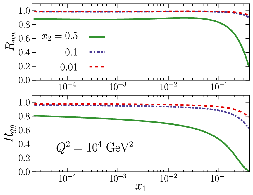
In figure 23(b) we show as a function of for three different values at high . Overall, the effect of the integration limit is not large, except at large . Indeed, at the kinematic limit the DPD should vanish, which is ensured by evolution even though it is not satisfied for our oversimplified starting conditions. Our exercise illustrates that even if one assumes that a DPD factorizes into the product of single parton distributions at some scale, this factorization cannot strictly hold at higher scales.
6.2 Independent partons and dependence
The ansatz (11) presented in section 4.1 assumes that the two partons are distributed independently of each other, even if for each of them we have correlations between longitudinal momentum and transverse position. It is natural to ask whether this form persists under evolution, provided that one is sufficiently far from the kinematic limit just discussed.
To answer this question is easy if one transforms both single and double parton distributions from transverse position to the Fourier conjugate transverse momentum. As was pointed out in [42], the convolution in (11) then turns into a simple product
| (31) |
The distributions in space do not have a probability interpretation since is a momentum difference between partons on the left- and right-hand sides of the final-state cut. This is discussed for instance in section 2.1 of [12] (where also the normalization factors in the Fourier transforms are specified). The ansatz (12) in impact parameter space turns into a Gaussian
| (32) |
in momentum space with an dependent width. We can now use the results of the previous subsection to conclude that for each the factorized form (31) will be preserved by evolution to higher scales to good accuracy as long as is not too close to . The convolution form (11) in transverse position space remains of course valid to the same extent.
7 Conclusions
Correlations between partons can have a large impact in double parton scattering processes, both on the overall cross section and on the distribution of particles in the final state. We have shown that the effect of double DGLAP evolution, where each of the two partons develops its own parton cascade, generally suppresses such correlations at higher scales. The strength of this suppression varies widely, with a rapid decrease of correlations in some cases and a slow decrease in others.
At a certain degree of accuracy, the dependence of DPDs on the transverse distance between the two partons is expected to depend on the type of the partons and on their momentum fractions. We have studied the evolution of a dependence motivated by the phenomenology of generalized parton distributions at the initial scale. We find that a Gaussian dependence at the initial scale is approximately preserved under evolution, with a noticeable but relatively slow change of the effective Gaussian width. Despite the mixing between gluons and quarks in the singlet sector, the differences between their distributions persist up to high scales.
Spin correlations between two partons in the proton are described by polarized DPDs. Positivity constrains these to be at most as large as the unpolarized DPDs for the same parton types, a property that is preserved under evolution to higher scales. For the initial conditions of evolution, we have either assumed maximum polarization or a degree of polarization as it is obtained when the two partons originate from the perturbative splitting of a single, unpolarized one. In the latter scenario, the degree of polarization strongly depends on the ratio of momentum fractions for certain parton combinations. We find that the DPDs for two longitudinally or two transversely polarized quarks decrease slowly with the evolution scale or even remain approximately constant. Given the rise of the corresponding unpolarized DPD, the degree of longitudinal or transverse quark polarization shows a rather pronounced decrease with . The DPD for two longitudinally polarized gluons rises slowly with the scale, as does the DPD for a longitudinally polarized gluon and a longitudinally polarized quark. However, due to the very rapid increase of unpolarized gluon distributions with , the degree of longitudinal polarization decreases with the scale both for and distributions, in particular at small . The distribution for two linearly polarized gluons decreases under evolution, and the associated degree of polarization quickly becomes negligible for below . In certain processes like double charm production, the DPD for one unpolarized and one linearly polarized gluon is relevant. Except at high , it increases with and the corresponding degree of polarization decreases rather gently. Our quantitative results in the gluon sector depend strongly on the initial scale of evolution and on the gluon densities used in the initial conditions, which entails a much stronger model dependence than for quarks. Broadly speaking, we find that almost all polarization effects become small for and , whereas for above a few many polarization correlations remain sizeable even at high scales.
The phase space available for parton radiation in DPDs is reduced compared with the case of single parton densities. As a result, evolution does not conserve the factorization of DPDs into separate functions of the momentum fractions and if one assumes this property at a certain scale. Quantitatively, we find that this effect is important only if at least one of the momentum fractions is of order or larger, otherwise one retains a factorized form to a good approximation. This result generalizes to the convolution ansatz specified in (11) because this ansatz corresponds to a product in the momentum space representation (31).
In summary, we find that the effect of scale evolution on parton correlations is important and should be included in quantitative estimates. The assumption that parton radiation will quickly wash out correlations is true in a few cases but cannot serve as a general guideline. How this affects double parton scattering processes remains to be studied in future work.
Acknowledgments
We are greatly indebted to J. Gaunt for the permission to use his DPD evolution code and for his help with all matters arising during its modification. We thank D. Boer for correspondence regarding references [27, 28, 29] and W. Vogelsang for calling to our attention the results in [30]. T.K. acknowledges financial support from the European Community under the “Ideas” program QWORK (contract 320389).
Appendix A Choice of single parton densities
The models we use for the initial conditions of unpolarized DPDs in sections 4, 5 and 6 are constructed from products of ordinary single parton distributions. For this we use LO PDFs, so as to match the leading-order evolution we perform for the DPDs. We need these PDFs at low scales, down to , where different PDF sets significantly deviate from each other.


This is clearly seen in figure 24, where we show LO PDFs from Alekhin (a02m_lo) [43], CTEQ6 (cteq6ll) [44], GJR (GJR08lo) [39] and MSTW (MSTW2008lo) [33]. We also show the dedicated Monte Carlo PDF set MRSTMCal [45]; the other set of that study (MRST2007lomod) looks similar. All PDF values are generated using the LHAPDF interface [46]. Not included in the figure are the LO PDFs of NNPDF2.1 [47] since they are not available at via LHAPDF. The CTEQ6 gluon distribution turns negative at low and is hence not suited for our purpose (one of our two models for polarized DPDs in section 5 builds on the positivity of parton distributions). For the same reason we discard the dedicated Monte Carlo PDFs of CT09 [48] (not shown here), although they are set to zero below some value of instead of going negative. The LO gluon distribution of HERAPDF1.5 [49] is very close to the one of CTEQ6 at (and hence not shown in the figure). It also turns negative at low .
Among the positive gluon PDFs shown in the figure, the sets of GJR08 and MSTW2008 represent extremes in the sense of having a very steep or a very flat behavior over a wide range. We chose these two sets for our investigations of DPDs, expecting that results obtained with different PDFs should approximately lie within the range covered by the two representatives we have selected. In the right panel of the figure we see that the spread of quark distributions in the different PDF sets is notable, but not as large as for the gluons.
For the evolution of DPDs, we adjusted the values of and of the quark masses to those used by the two PDF sets we have selected. This is
| (33) | ||||||||
| for GJR and | ||||||||
| (34) | ||||||||
for MSTW.
Appendix B Double parton distributions from perturbative splitting
For small interparton distances , or more precisely in the limit , where is a typical hadronic scale, the dominant contribution to DPDs is given by the short-distance splitting of a single parton into two [12]. To leading order in , one can then express the DPD as the product of a usual PDF with an expression for the perturbative splitting; at higher orders the product turns into a convolution. From the results of section 5.2 in [12] we can readily extract the corresponding expressions for the collinear color-singlet DPDs we are studying in the present work.
For unpolarized or doubly polarized DPDs, we have at leading order in
| (35) |
from the splitting process , with kernels
| (36) | ||||||||
where . Corrections to (35) are suppressed by further powers of or by powers of . In , and we recognize the familiar DGLAP splitting functions for . Further DPDs are obtained by permuting the parton labels and momentum fractions. All other unpolarized or doubly polarized distributions, including , do not receive any contribution from perturbative splitting at this accuracy.
DPDs with one polarized and one unpolarized parton arise by perturbative splitting only for linearly polarized gluons,
| (37) |
with
| (38) |
Because and are multiplied by two vectors in their definitions, the associated distributions and diverge like for , just as the distributions in (35). The distributions and do not receive contributions from perturbative splitting due to the chiral invariance of massless QCD.
References
- (1) P. Bartalini et al., Multi-Parton Interactions at the LHC, arXiv:1111.0469.
- (2) S. Plätzer and M. Diehl, Proceedings MPI@LHC 2011, DESY-PROC-2012-03, doi:10.3204/DESY-PROC-2012-03.
- (3) H. Abramowicz et al., Summary of the Workshop on Multi-Parton Interactions (MPI@LHC 2012), arXiv:1306.5413.
- (4) R. Kirschner, Generalized Lipatov-Altarelli-Parisi Equations and Jet Calculus Rules, Phys. Lett. B 84 (1979) 266.
- (5) V. P. Shelest, A. M. Snigirev and G. M. Zinovev, The Multiparton Distribution Equations in QCD, Phys. Lett. B 113 (1982) 325.
- (6) A. M. Snigirev, Double parton distributions in the leading logarithm approximation of perturbative QCD, Phys. Rev. D 68 (2003) 114012 [hep-ph/0304172].
- (7) J. R. Gaunt and W. J. Stirling, Double Parton Distributions Incorporating Perturbative QCD Evolution and Momentum and Quark Number Sum Rules, JHEP 1003 (2010) 005 [arXiv:0910.4347].
- (8) F. A. Ceccopieri, An update on the evolution of double parton distributions, Phys. Lett. B 697 (2011) 482 [arXiv:1011.6586].
- (9) J. R. Gaunt and W. J. Stirling, Double Parton Scattering Singularity in One-Loop Integrals, JHEP 1106 (2011) 048 [arXiv:1103.1888].
- (10) J. R. Gaunt, Single Perturbative Splitting Diagrams in Double Parton Scattering, JHEP 1301 (2013) 042 [arXiv:1207.0480].
- (11) M. Diehl and A. Schäfer, Theoretical considerations on multiparton interactions in QCD, Phys. Lett. B 698 (2011) 389 [arXiv:1102.3081].
- (12) M. Diehl, D. Ostermeier and A. Schäfer, Elements of a theory for multiparton interactions in QCD, JHEP 1203 (2012) 089 [arXiv:1111.0910].
- (13) M. G. Ryskin and A. M. Snigirev, A Fresh look at double parton scattering, Phys. Rev. D 83 (2011) 114047 [arXiv:1103.3495].
- (14) A. V. Manohar and W. J. Waalewijn, What is Double Parton Scattering?, Phys. Lett. B 713 (2012) 196 [arXiv:1202.5034].
- (15) B. Blok, Yu. Dokshitzer, L. Frankfurt and M. Strikman, pQCD physics of multiparton interactions, Eur. Phys. J. C 72 (2012) 1963 [arXiv:1106.5533].
- (16) B. Blok, Yu. Dokshitzer, L. Frankfurt and M. Strikman, Perturbative QCD correlations in multi-parton collisions, arXiv:1306.3763.
- (17) M. Diehl, Correlation effects in multiple hard scattering, arXiv:1306.6480.
- (18) M. Mekhfi, Multiparton Processes: An Application To Double Drell-Yan, Phys. Rev. D 32 (1985) 2371.
- (19) M. Mekhfi, Correlations in Color and Spin in Multiparton Processes, Phys. Rev. D 32 (1985) 2380.
- (20) H. -M. Chang, A. V. Manohar and W. J. Waalewijn, Double Parton Correlations in the Bag Model, Phys. Rev. D 87 (2013) 3, 034009 [arXiv:1211.3132].
- (21) A. V. Manohar and W. J. Waalewijn, A QCD Analysis of Double Parton Scattering: Color Correlations, Interference Effects and Evolution, Phys. Rev. D 85 (2012) 114009 [arXiv:1202.3794].
- (22) T. Kasemets, Double parton scattering — a tale of two partons, DESY-THESIS-2013-035.
- (23) M. Diehl and T. Kasemets, Positivity bounds on double parton distributions, JHEP 1305 (2013) 150 [arXiv:1303.0842].
- (24) T. Kasemets and M. Diehl, Angular correlations in the double Drell-Yan process, JHEP 1301 (2013) 121 [arXiv:1210.5434].
- (25) C. Bourrely, J. Soffer, F. M. Renard and P. Taxil, Spin Effects At Supercollider Energies, Phys. Rept. 177 (1989) 319.
- (26) R. L. Jaffe and N. Saito, QCD selection rules in polarized hadron collisions, Phys. Lett. B 382 (1996) 165 [hep-ph/9604220].
- (27) D. Boer, P. J. Mulders and C. Pisano, Dijet imbalance in hadronic collisions, Phys. Rev. D 80 (2009) 094017 [arXiv:0909.4652].
- (28) D. Boer, S. J. Brodsky, P. J. Mulders and C. Pisano, Direct Probes of Linearly Polarized Gluons inside Unpolarized Hadrons, Phys. Rev. Lett. 106 (2011) 132001 [arXiv:1011.4225].
- (29) J.-W. Qiu, M. Schlegel and W. Vogelsang, Probing Gluonic Spin-Orbit Correlations in Photon Pair Production, Phys. Rev. Lett. 107 (2011) 062001 [arXiv:1103.3861].
- (30) W. Vogelsang, evolution of spin dependent parton densities, Acta Phys. Polon. B 29 (1998) 1189 [hep-ph/9805295].
- (31) J. Gaunt, Double parton scattering in proton-proton collisions, Thesis, University of Cambridge (2012), https://www.repository.cam.ac.uk/handle/1810/243945
- (32) R. K. Ellis, W. J. Stirling and B. R. Webber, Camb. Monogr. Part. Phys. Nucl. Phys. Cosmol. 8 (1996) 1.
- (33) A. D. Martin, W. J. Stirling, R. S. Thorne and G. Watt, Parton distributions for the LHC, Eur. Phys. J. C 63 (2009) 189 [arXiv:0901.0002].
- (34) M. Diehl, T. Feldmann, R. Jakob and P. Kroll, Eur. Phys. J. C 39, 1 (2005) [hep-ph/0408173].
- (35) M. Diehl and W. Kugler, Some numerical studies of the evolution of generalized parton distributions, Phys. Lett. B 660, 202 (2008) [arXiv:0711.2184].
- (36) A. Aktas et al. [H1 Collaboration], Elastic production at HERA, Eur. Phys. J. C 46, 585 (2006) [hep-ex/0510016].
- (37) F. D. Aaron et al. [H1 Collaboration], Measurement of deeply virtual Compton scattering and its -dependence at HERA, Phys. Lett. B 659, 796 (2008) [arXiv:0709.4114].
- (38) M. Botje, QCDNUM: Fast QCD Evolution and Convolution, Comput. Phys. Commun. 182 (2011) 490 [arXiv:1005.1481].
- (39) M. Glück, P. Jimenez-Delgado and E. Reya, Dynamical parton distributions of the nucleon and very small-x physics, Eur. Phys. J. C 53 (2008) 355 [arXiv:0709.0614].
- (40) M. Rinaldi, S. Scopetta and V. Vento, Double parton correlations in constituent quark models, Phys. Rev. D 87 (2013) 114021 [arXiv:1302.6462].
- (41) W. Broniowski and E. R. Arriola, Valence double parton distributions of the nucleon in a simple model, arXiv:1310.8419.
- (42) B. Blok, Yu. Dokshitzer, L. Frankfurt and M. Strikman, The four jet production at LHC and Tevatron in QCD, Phys. Rev. D 83 (2011) 071501 [arXiv:1009.2714].
- (43) S. Alekhin, Parton distributions from deep inelastic scattering data, Phys. Rev. D 68 (2003) 014002 [hep-ph/0211096].
- (44) J. Pumplin et al., New generation of parton distributions with uncertainties from global QCD analysis, JHEP 0207 (2002) 012 [hep-ph/0201195].
- (45) A. Sherstnev and R. S. Thorne, Different PDF approximations useful for LO Monte Carlo generators, arXiv:0807.2132.
- (46) http://lhapdf.hepforge.org
- (47) R. D. Ball et al. [NNPDF Collaboration], Unbiased global determination of parton distributions and their uncertainties at NNLO and at LO, Nucl. Phys. B 855 (2012) 153 [arXiv:1107.2652].
- (48) H.-L. Lai et al., Parton Distributions for Event Generators, JHEP 1004 (2010) 035 [arXiv:0910.4183].
- (49) H1 and ZEUS Collaborations, HERAPDF1.5LO PDF Set with Experimental Uncertainties, H1prelim-13-141 and ZEUS-prel-13-003, http://www-h1.desy.de/h1/www/publications/H1_sci_results.shtml