Monte Carlo computation of the Vassiliev knot invariant of degree 2 in the integral representation

There are many situations in which it is necessary to distinguish the topological properties of ring-shaped quasi one-dimensional objects. This is for instance the case of polymers [1, 2], vortex structures in nematic liquid crystals [3], ${}^{3}He$ superfluid [4] and disclination lines in chiral nematic colloids [5]. In order to ascertain the type of a knot, it is possible to apply the so-called knot invariants. These mathematical quantities, which remain unchanged under ambient isotopy, are usually represented in the form of polynomials, like for example the Alexander [6] or the HOMFLY polynomials [7]. Alternatively, certain knot invariants may be defined in terms of multiple curvilinear integrals, in which the integrations are performed along the spatial trajectory of the knot or elements of it [8, 9, 10]. Particularly important for applications is the case in which knots are constructed by joining together at their ends a set of $N$ segments. Discrete knots of this kind are in fact the most common concrete realizations of knots in numerical simulations. Formally, a discrete knot is $C^{0}-$curve which is piecewise smooth and is characterized by sharp corners at the joints between contiguous segments. While there exist already well established mathematical algorithms in order to compute numerically polynomial knot invariants, see for instance the pioneering work [11], there are not many studies concerning the numerical computation of knot invariants given in the form of multiple line integrals for such discrete knots. Of course, the calculation of line integrals over discrete data is a textbook subject [12, 13]. Moreover, problems in which knots are discretized using splines, have been investigated for example in [14]. However, we are faced with a somewhat different problem, which arises due to the fact that knot invariants expressed as multiple curvilinear integrals are not well defined in the case of discrete knots. The reason of this failure is related to the presence of the non-smooth corners at the joints between two contiguous segments. As a consequence, the main goal pursued here is to replace the piecewise smooth curves representing a discrete knot with more regular ones. To obtain a smoothing algorithm that is able to perform this replacement for general discrete knots without destroying their topology, a strategy has been adopted that can be briefly summarized as follows. First, the sharp corners are surrounded with spheres whose radii are chosen in such a way that they do not intersect with themselves and with other elements of the knot. After that, the elements containing the corners inside the spheres are substituted with arcs of smooth curves. This procedure transforms the original trajectories into $G^{1}-$curves¹¹ 1 We recall that a $G^{1}-$curve is a tangent vector geometrically continuous curve characterized by the fact that the unit tangent vector to the curve is continuous [15]. without altering their topological configurations. As an application, the case of the Vassiliev knot invariant of degree 2 [16] of a knot $C$, denoted here $\varrho(C)$, is worked out. The main advantages of choosing this invariant are its relative simplicity and the fact that its exact values for different knots can be computed analytically. In this way, it is possible to perform a comparison between numerical and analytical results. After the smoothing procedure proposed in this work, it becomes possible to calculate $\varrho(C)$ numerically with an arbitrarily high precision.

Despite its simplicity, the Vassiliev invariant of degree 2 requires the evaluation of complicated quadruple and triple line integrals. Having in mind concrete applications, in which the knot invariant $\varrho(C)$ must be computed millions of times, see for instance Ref. [17], we have proposed here several strategies to accelerate its calculation. It turns out that Monte Carlo integration algorithms are faster than traditional integration methods [18]. For this reason, a Monte Carlo integration scheme is adopted and explained in details. Moreover, several tricks to speed up the computation of $\varrho(C)$, that are specific to particular applications or situations, are presented. Since the time for evaluating $\varrho(C)$ is sensitive to the number of segments $N$ composing the knot, but not on its length, we have provided an algorithm to reduce by a factor three the number of segments without changing the topology of the knot. This algorithm is valid for knots defined on a simple cubic lattice. Secondly, it is shown that the number of points of the trajectory $C$ to be sampled during the Monte Carlo integration procedure may be considerably decreased when the knot invariant $\varrho(C)$ is used in order to detect topology changes that may potentially occur after a random transformation of an element of the trajectory of the knot. Such random transformations, like for instance the pivot moves [19], the pull moves [20] and the BFACF moves [21], are extensively exploited in numerical simulations of polymer knots.

The material presented in this paper is divided as follows. In the next Section, the Vassiliev invariant of degree 2 is defined in the case of general smooth curves. In Section III we specialize to general discrete knots, which are represented as piecewise smooth curves parametrized by a continuous variable $S\in[0,N]$. In this way, the calculation of $\varrho(C)$ is reduced to that of multiple integrals over a set of variables $S,T,U,V\in[0,N]$ and can be tackled by standard Monte Carlo techniques. A numerical version of the so-called framing [22] procedure is implemented in order to regularize singularities that are possibly arising in some of the terms to be integrated. While it is analytically proven that the sum of all these terms is always finite, the presence of singularities in single terms may spoil the result of the numerical integration. A smoothing procedure is presented in Section IV in order to transform a general discrete knot into a $G^{1}-$curve. This procedure allows the calculation of $\varrho(C)$ by Monte Carlo integration techniques with an arbitrary precision depending on the number of used samples. In Section V a few methods to speed up the calculations are discussed. Finally, the conclusions are drawn in Section VI.

Let us consider a general knot of length $L$ in the flat three dimensional space $\mathbb{R}^{3}$ spanned by a set of cartesian coordinates $\boldsymbol{x}=(x^{1},x^{2},x^{3})$. The space indexes are labeled with greek letters $\mu,\nu,\rho,\ldots=1,2,3$. The Alexander-Briggs notation for denoting knots is used. In this Section, the spatial trajectory $C$ formed in the space by the knot is chosen to be a smooth curve $\boldsymbol{x}(s):[0,L]\longrightarrow\mathbb{R}^{3}$ parametrized using its arc-length $0\leq s\leq L$. Different points on the curve corresponding to different values of the arc-length $s,t,u$ and $v$ will be denoted with the symbols $x^{\mu}(s),y^{\nu}(t),z^{\rho}(u)$ and $w^{\sigma}(v)$, with $\mu,\nu,\rho,\sigma=1,2,3$. As a convention, summation over repeated indexes is understood. Moreover, let $\dot{x}^{\mu}(s)$ be the derivative of $x^{\mu}(s)$ with respect to $s$. An analogous notation holds for $\dot{y}^{\nu}(t),\dot{z}^{\rho}(u)$ and $\dot{w}^{\sigma}(v)$. Finally, $\epsilon_{\mu\nu\rho}$ is the completely antisymmetric tensor uniquely defined by the condition $\epsilon_{123}=1$.

With the above settings, the Vassiliev knot invariant of degree 2 $\varrho(C)$ of a knot $C$ can be written as follows [9, 10, 23]:

$$\varrho(C)=\varrho_{1}(C)+\varrho_{2}(C)$$

(1)

where $\varrho_{1}(C)$ and $\varrho_{2}(C)$ are two path ordered multiple line integrals given by:

$$\varrho_{1}(C)=\int_{0}^{L}ds\int_{0}^{s}dt\int_{0}^{t}duF_{1}(\boldsymbol{x}(s),\boldsymbol{y}(t),\boldsymbol{z}(u);\dot{\boldsymbol{x}}(s),\dot{\boldsymbol{y}}(t),\dot{\boldsymbol{z}}(u))$$

(2)

and

$$\varrho_{2}(C)=\int_{0}^{L}ds\int_{0}^{s}dt\int_{0}^{t}du\int_{0}^{u}dvF_{2}(\boldsymbol{x}(s),\boldsymbol{y}(t),\boldsymbol{z}(u),\boldsymbol{w}(v);\dot{\boldsymbol{x}}(s),\dot{\boldsymbol{y}}(t),\dot{\boldsymbol{z}}(u),\dot{\boldsymbol{w}}(v))$$

(3)

The quantities $F_{1}$ and $F_{2}$ are defined below:

	$\displaystyle-32\pi^{3}F_{1}(\boldsymbol{x},\boldsymbol{y},\boldsymbol{z};\dot{\boldsymbol{x}},\dot{\boldsymbol{y}},\dot{\boldsymbol{z}})$	$\displaystyle=$	$\displaystyle C_{1}C_{2}C_{3}\left[\dot{\boldsymbol{y}}\cdot\dot{\boldsymbol{z}}(\dot{\boldsymbol{x}}\cdot\boldsymbol{c})+\dot{\boldsymbol{x}}\cdot\dot{\boldsymbol{z}}(\dot{\boldsymbol{y}}\cdot\boldsymbol{b})+\dot{\boldsymbol{x}}\cdot\dot{\boldsymbol{y}}(\dot{\boldsymbol{z}}\cdot\boldsymbol{a})\right]$		(4)
		$\displaystyle-$	$\displaystyle C_{1}C_{2}^{2}C_{3}\left[\dot{\boldsymbol{y}}\cdot(\boldsymbol{a}\times\boldsymbol{b})\left(\boldsymbol{a}+\boldsymbol{b}\frac{a}{b}\right)\cdot(\dot{\boldsymbol{z}}\times\dot{\boldsymbol{x}})\right.$
		$\displaystyle+$	$\displaystyle\left.\dot{\boldsymbol{z}}\cdot(\boldsymbol{a}\times\boldsymbol{b})\left(\boldsymbol{b}+\boldsymbol{a}\frac{b}{a}\right)\cdot(\dot{\boldsymbol{y}}\times\dot{\boldsymbol{x}})\right]$
		$\displaystyle+$	$\displaystyle C_{1}C_{2}\left[\dot{\boldsymbol{y}}\cdot(\boldsymbol{a}\times\boldsymbol{b})\left(\boldsymbol{b}\frac{c-a}{b^{2}}+\boldsymbol{c}\frac{a+b}{c^{2}}\right)\cdot(\dot{\boldsymbol{z}}\times\dot{\boldsymbol{x}})\right.$
		$\displaystyle+$	$\displaystyle\left.\dot{\boldsymbol{z}}\cdot(\boldsymbol{a}\times\boldsymbol{b})\left(\boldsymbol{a}\frac{c-b}{a^{2}}-\boldsymbol{c}\frac{a+b}{c^{2}}\right)\cdot(\dot{\boldsymbol{y}}\times\dot{\boldsymbol{x}})\right]$

$\displaystyle F_{2}(\boldsymbol{x},\boldsymbol{y},\boldsymbol{z},\boldsymbol{w};\dot{\boldsymbol{x}},\dot{\boldsymbol{y}},\dot{\boldsymbol{z}},\dot{\boldsymbol{w}})$

$\displaystyle=$

$\displaystyle\frac{1}{8\pi^{2}}\left(\dot{\boldsymbol{x}\cdot}\left(\dot{\boldsymbol{z}}\times\frac{\boldsymbol{b}}{b^{3}}\right)\right)\left(\dot{\boldsymbol{y}\cdot}\left(\dot{\boldsymbol{w}}\times\frac{\boldsymbol{c}}{c^{3}}\right)\right)$

(5)

In Eqs. (4) and (5) we have put:

$$\boldsymbol{a}=\boldsymbol{y}-\boldsymbol{x}\qquad\boldsymbol{b}=\boldsymbol{z}-\boldsymbol{x}\qquad\boldsymbol{c}=\boldsymbol{y}-\boldsymbol{z}$$

(6)

and

	$\displaystyle C_{1}$	$\displaystyle=$	$\displaystyle\frac{2\pi}{abc}$		(7)
	$\displaystyle C_{2}$	$\displaystyle=$	$\displaystyle\frac{1}{ab+a_{\mu}b_{\mu}}$		(8)
	$\displaystyle C_{3}$	$\displaystyle=$	$\displaystyle a+b-c$		(9)

Let us note that in Eq. (8) we have used a convention for which repeated indexes are summed. It is known that the above defined $\varrho(C)$ is related to the second coefficient $a_{2}(C)$ of the Conway polynomial of a knot $C$ through the following relation [10]:

$$a_{2}(C)=\dfrac{1}{2}\left[\varrho(C)+\dfrac{1}{12}\right]$$

(10)

The coefficients of the Conway polynomials can be computed analytically for every knot topology. $\varrho(C)$ is the simplest knot invariant expressed in the form of contour integrals. It is also called the Casson knot invariant, see Ref. [24]

In principle, analytical computations of $\varrho(C)$ are possible if the curve $\boldsymbol{x}(s)$ describing the knot $C$ is given in parametric form. However, a close expression of $\boldsymbol{x}(s)$ for a knot of arbitrary shape usually does not exist and one should pass to a discrete representation of it. To switch from continuous functions to discrete ones is one of the most standard problems of numerical integration. In the present case, the situation is opposite. For instance, in numerical simulations involving ring-shaped objects with nontrivial topological configurations the knots are already discrete by construction. The real difficulty is rather that knot invariants expressed in the form of multiple line integrals like $\varrho(C)$, cease to be topological invariants if knots are discrete. In order to restore this invariance, a procedure that is able to smooth up a discrete knot transforming it from a $C^{0}-$curve into a $G^{1}-$curve without destroying its topological configuration is needed. Such a procedure will be presented in the following.

First of all, to be concrete, let us define the discrete knot as a set of $N$ points:

$$\boldsymbol{x}_{i}=\boldsymbol{x}(s_{i})\qquad\qquad\left\{\begin{array}[]{c}i=1,\ldots,N\\ 0<s_{1}<s_{2}\cdots<s_{N}=L\end{array}\right.$$

(11)

joined together by $N$ segments

	$\displaystyle\boldsymbol{l}_{i}$	$\displaystyle=$	$\displaystyle\boldsymbol{x}_{i}-\boldsymbol{x}_{i-1}\qquad\qquad i=2,\ldots,N$		(12)
	$\displaystyle\boldsymbol{l}_{1}$	$\displaystyle=$	$\displaystyle\boldsymbol{x}_{1}-\boldsymbol{x}_{N}$		(13)

The discrete knot may be regarded as a piecewise smooth curve $\boldsymbol{X}(S):[0,N]\longrightarrow\mathbb{R}$, where

$$0\leq S\leq N$$

(14)

Explicitly, a general point located on the $i-$th segment of $\boldsymbol{X}(S)$ is identified by the relations:

$$\boldsymbol{X}(S)=\boldsymbol{x}_{i-1}+(S-[S])\boldsymbol{l}_{i}\qquad\left\{\begin{array}[]{c}i-1<S\leq i\\ i=2,\ldots,N\end{array}\right.$$

(15)

and

$$\boldsymbol{X}(S)=\boldsymbol{x}_{N}+(S-[S])\boldsymbol{l}_{1}\qquad 0<S\leq 1$$

(16)

In the above equations $[S]$ denotes the integer part of $S$. The example of a curve $\boldsymbol{X}(S)$ with eight segments is given in Fig. 1. In the limit in which $N$ approaches infinity and the lengths of the $N$ segments become vanishingly small, a continuous representation of the knot is obtained. If $l_{i}=|\boldsymbol{l}_{i}|$ denotes the length of the $i-$th segment and $\Lambda_{N}=\sum_{i=1}^{N}l_{i}$ is the total length of the discretized curve, then the length $L$ of the continuous knot is given by:

$$\lim_{\begin{subarray}{c}N\to\infty\\ l_{i}\to 0,\,i=1,\ldots,N\end{subarray}}\Lambda_{N}=L$$

(17)

At this point it is possible to compute the contributions $\varrho_{1}(C)$ and $\varrho_{2}(C)$ to the Vassiliev invariant of degree 2 for a general discrete knot $C$ with trajectory $\boldsymbol{X}(S)$. With the above definitions, the same prescriptions of Eqs. (2) and (3), which are valid for a smooth curve $\boldsymbol{x}(s)$, can be formally applied. It is sufficient to substitute the smooth trajectories $\boldsymbol{x}(s),\boldsymbol{y}(t),\boldsymbol{z}(u)$ and $\boldsymbol{w}(v)$ with their discrete analogs $\boldsymbol{X}(S),\boldsymbol{Y}(T),\boldsymbol{Z}(U)$ and $\boldsymbol{W}(V)$. In the following, the symbols $F_{1}(S,T,U)$ and $F_{2}(S,T,U,V)$ will denote the integrands of Eqs. (2) and (3) in the case of a discrete knot in which the variables $s,t,u,v$ are replaced by $S,T,U,V$. Of course, in these equations the upper integration boundary $L$ should be replaced by $N$. The derivatives $\dot{\boldsymbol{X}}(S),\dot{\boldsymbol{Y}}(T),\dot{\boldsymbol{Z}}(U)$ and $\dot{\boldsymbol{W}}(V)$ require some more care. On the $i-$th segment, away from the joints, the curve is trivially smooth and the computation of $\dot{\boldsymbol{X}}(S),\dot{\boldsymbol{Y}}(T),\dot{\boldsymbol{Z}}(U),\dot{\boldsymbol{W}}(V)$ is straightforward:

	$\displaystyle\dot{\boldsymbol{X}}(S)$	$\displaystyle=$	$\displaystyle\boldsymbol{l}_{i}\qquad\left\{\begin{array}[]{c}i-1<S<i\\ i=2,\ldots,N\end{array}\right.$
	$\displaystyle\dot{\boldsymbol{X}}(S)$	$\displaystyle=$	$\displaystyle\boldsymbol{l}_{1}\qquad 0<S<1$		(21)

At the points $\boldsymbol{x}_{1},\ldots,\boldsymbol{x}_{N}$ in which the segments join together, instead, the curve $\boldsymbol{X}(S)$ ceases to be differentiable. Still, it is possible to define formally the derivatives at these points by assuming that the tangent to the discrete trajectory in $\boldsymbol{x}_{i-1}$ is proportional to the segment $\boldsymbol{l}_{i}$. Using this convention we obtain:

	$\displaystyle\dot{\boldsymbol{X}}(i-1)$	$\displaystyle=$	$\displaystyle\boldsymbol{l}_{i}\qquad\qquad i=2,\ldots,N$		(22)
	$\displaystyle\dot{\boldsymbol{X}}(N)$	$\displaystyle=$	$\displaystyle\boldsymbol{l}_{1}$		(23)

The above definition is clearly not unique. Analogously, we could have chosen $\dot{\boldsymbol{X}}(i-1)=\boldsymbol{l}_{i-1}$, $i=2,\ldots,N$ and $\dot{\boldsymbol{X}}(N)=\boldsymbol{l}_{N}$.

With the prescriptions (14–16) and (III–23) given above in order to parametrize the discrete knot, the evaluation of the two multiple line integrals appearing in Eqs. (2) and (3) may be performed using numerical integration techniques like the rectangle rule method, trapezoidal rule method, Simpson’s rule method, Newton-Cotes method, Romberg method, Gauss method etc. [25] Let us note that the variables $S,T$ and $U$ appearing in $\varrho_{1}(C)$, see Eq. (2), span a space of volume

$$V_{1}=\frac{N^{3}}{6}$$

(24)

while the variables $S,T,U$ and $V$ appearing in Eq. (3) span a space of volume

$$V_{2}=\frac{N^{4}}{24}$$

(25)

When $N$ is large, these volumes become too large to be treated with quadrature methods and it is more convenient to compute the right hand sides of Eqs. (2) and (3) using a Monte Carlo approach²² 2 Nonstandard methods like that based on Particle Swarm Optimization proposed in [25] could probably also be applied successfully.. For the integral of a function of $m$ variables $f(\xi_{1},\cdots,\xi_{m})$ with integration boundaries like those in Eqs. (2) and (3), it can be applied to this purpose the general formula:

	$\displaystyle\int_{a_{1}}^{b_{1}}d\xi_{1}\int_{a_{2}}^{\xi_{1}}d\xi_{2}\cdots\int_{a_{m}}^{\xi_{m-1}}d\xi_{m}f(\xi_{1},\cdots,\xi_{m})$
	$\displaystyle\approx\dfrac{1}{n}\left[\sum_{i=1}^{n}f(\xi_{1}^{(i)},\cdots,\xi_{m}^{(i)})(b_{1}-a_{1})\prod_{\sigma=2}^{m}(\xi_{\sigma}^{(i)}-a_{\sigma})\right]$		(26)

where the $\xi_{\sigma}^{(i)}$’s, $i=1,\cdots,n$ and $\sigma=1,\cdots,m$ denote randomly chosen variables in the range:

$$\begin{array}[]{ccl}[a_{1},b_{1}]&\mbox{when}&\sigma=1\\ {[a_{\sigma},\xi_{\sigma}]}&\mbox{when}&\sigma=2,\ldots,m\end{array}$$

(27)

The naive procedure discussed above is plagued by two systematic errors. First of all, the discrete knots treated here so far are not smooth at the joints between two segments. On a simple cubic lattice, it is possible to verify that the values of $\varrho(C)$ computed for a discrete knot are always greater than the analytical values, a fact that is certainly related to the presence of sharp corners at these joints. This excess from the exact value is roughly proportional to the number of the corners. The second source of errors is connected with possible singularities arising in the integrands $F_{1}(S,T,U)$ and $F_{2}(S,T,U,V)$ appearing in Eqs. (2) and (3). Of course, globally both $F_{1}(S,T,U)$ and $F_{2}(S,T,U,V)$ are regular for every value of $S,T,U$ and $V$ as it has been proved in [10]. However, the fact that $F_{1}(S,T,U)$ and $F_{2}(S,T,U,V)$ are finite everywhere does not prevent the presence of singularities in single terms entering in the expressions of these integrands. Looking at Eqs. (4–9), it is easy to realize that some of these terms diverge whenever one or more of the following conditions are met:

	$\displaystyle\boldsymbol{Y}(T)-\boldsymbol{X}(S)$	$\displaystyle=$	$\displaystyle 0$		(28)
	$\displaystyle\boldsymbol{Z}(U)-\boldsymbol{X}(S)$	$\displaystyle=$	$\displaystyle 0$		(29)
	$\displaystyle\boldsymbol{Y}(T)-\boldsymbol{Z}(U)$	$\displaystyle=$	$\displaystyle 0$		(30)
	$\displaystyle|\boldsymbol{Y}(T)-\boldsymbol{X}(S)|\,|\boldsymbol{Z}(U)-\boldsymbol{X}(S)|+(\boldsymbol{Y}(T)-\boldsymbol{X}(S))\cdot(\boldsymbol{Z}(U)-\boldsymbol{X}(S))$	$\displaystyle=$	$\displaystyle 0$		(31)

When summed together, these singularities disappear making $F_{1}(S,T,U)$ and $F_{2}(S,T,U,V)$ finite, but for the purposes of numerical calculations a regularization is needed to remove them. To this purpose, a suitable regularization is the framing of the trajectories described in [22]. In the present context, the framing consists in a slight deformation of the curves $\boldsymbol{X}(S)$, $\boldsymbol{Y}(T)$, $\boldsymbol{Z}(U)$ and $\boldsymbol{W}(V)$ of the kind:

	$\displaystyle X^{\mu}(S)$	$\displaystyle\longrightarrow$	$\displaystyle X_{\epsilon_{X}}^{\mu}(S)=X^{\mu}(S)+\epsilon n^{\mu}(S)$		(32)
	$\displaystyle Y^{\nu}(T)$	$\displaystyle\longrightarrow$	$\displaystyle Y_{\epsilon_{Y}}^{\nu}(T)=Y^{\nu}(T)+2\epsilon n^{\nu}(T)$		(33)
	$\displaystyle Z^{\rho}(U)$	$\displaystyle\longrightarrow$	$\displaystyle Z_{\epsilon_{Z}}^{\rho}(U)=Z^{\rho}(U)+3\epsilon n^{\rho}(U)$		(34)
	$\displaystyle W^{\sigma}(V)$	$\displaystyle\longrightarrow$	$\displaystyle W_{\epsilon_{W}}^{\sigma}(V)=W^{\sigma}(V)+4\epsilon n^{\sigma}(V)$		(35)

where $n^{\mu}(S),n^{\nu}(T),n^{\rho}(U)$ and $n^{\sigma}(V)$ denote unit vectors normal to the trajectories $\boldsymbol{X}(S)$, $\boldsymbol{Y}(T)$, $\boldsymbol{Z}(U)$ and $\boldsymbol{W}(V)$ respectively. $\epsilon$ is a very small parameter. Clearly, the prescription provided in Eqs. (32–35) is able to remove the divergences at the locations defined in (28–31). Moreover, in the limit $\epsilon\to 0$ one recovers the exact expression of $\varrho(C)$ independently of the choice of the normal unit vectors $n^{\mu}(S),n^{\nu}(T),n^{\rho}(U)$ and $n^{\sigma}(V)$ as it has been proved in Ref. [10]. For example, in calculations on a simple cubic lattice the framing can be implemented by small shifts of the trajectories $\boldsymbol{X}(S)$, $\boldsymbol{Y}(T)$, $\boldsymbol{Z}(U)$ and $\boldsymbol{W}(V)$ along the direction $(1,1,1)$. This is sufficient to regularize all potentially divergent terms in $F_{1}(S,T,U)$ and $F_{2}(S,T,U,V)$ without creating dangerous intersections of the trajectories of the shifted knots that are forbidden. From our simulations it turns out that the results of the computations of $\varrho(C)$ are not much sensitive to the values of the $\epsilon-$parameter. This is connected to the fact that the points in which the singularity conditions of Eqs. (28–31) are satisfied represent a very small subset of the set of all sampled points.

To eliminate the systematic error due to the presence of the sharp corners is much more difficult. This will be the subject of the next Section, in which a smoothing procedure will be presented, that transforms the curve $\boldsymbol{X}(S)$ into a curve whose first derivatives exist and are continuous.

The effect of the sharp corners at the joints of the segments on the computation of $\varrho(C)$ can be checked using the very simple example of an unknot with two different trajectories:

• •

  A smooth circle defined by the parametric curve $x^{1}(\theta)=\cos(\theta)$, $x^{2}(\theta)=\sin(\theta)$ and $x^{3}(\theta)=0$, $\theta\in[0,2\pi]$, see Fig. 2(a).

• •

  A square defined on a simple cubic lattice as shown in Fig. 2(b).

The exact value of the Vassiliev invariant of degree 2 for the unknot is $-\frac{1}{12}\sim-0.083$. The Monte Carlo computation of $\varrho(C)$ gives a result that is very near to the exact one in the case of the circle: $\varrho(C)=-0.083\pm 1.72\times 10^{-4}$. However, for the square we obtain $\varrho(C)=0.050\pm 1.17\times 10^{-4}$, which is far from the expected result. To avoid these ambiguities in the calculation of $\varrho(C)$ for discrete knots, a smoothing procedure for eliminating the sharp corners will be presented.

The idea is to replace at each of the joints $\boldsymbol{x}_{i}$ the neighborhoods of the corners with smooth arcs of curves whose ends are glued together in such a way that the whole knot will be a continuous curve with its first derivative. To illustrate the method, we pick up a triplet of contiguous segments $\boldsymbol{l}_{i-1},\boldsymbol{l}_{i}$ and $\boldsymbol{l}_{i+1}$, see Fig. 3.

It is easy to realize that the segment $\boldsymbol{l}_{i}$ is shared by the two corners centered at the points $\boldsymbol{x}_{i-1}$ and $\boldsymbol{x}_{i}$. This is not desirable for our purposes. To achieve the goal that each corner will be subtended by couples of segments that are not in common with those related to other corners, we divide each segment $\boldsymbol{l}_{i}$, $i=1,\ldots,N$, into the three subsegments:

	$\displaystyle\boldsymbol{l}_{i}^{-}$	$\displaystyle=$	$\displaystyle\boldsymbol{x}_{i}^{-}-\boldsymbol{x}_{i-1}$		(36)
	$\displaystyle\boldsymbol{l}_{i}^{0}$	$\displaystyle=$	$\displaystyle\boldsymbol{x}_{i}^{+}-\boldsymbol{x}_{i}^{-}$		(37)
	$\displaystyle\boldsymbol{l}_{i}^{+}$	$\displaystyle=$	$\displaystyle\boldsymbol{x}_{i}^{+}-\boldsymbol{x}_{i}$		(38)

The ends $\boldsymbol{x}_{i}^{-}$ and $\boldsymbol{x}_{i}^{+}$ are fixed in such a way that the lengths of $\boldsymbol{l}_{i}^{-},\boldsymbol{l}_{i}^{0}$ and $\boldsymbol{l}_{i}^{+}$ are $d_{i-1}^{\prime}$, $l_{i}-d_{i-1}^{\prime}-d_{i}$ and $d_{i}$ respectively (see Fig. 4):

	$\displaystyle\boldsymbol{x}_{i}^{-}$	$\displaystyle=$	$\displaystyle\boldsymbol{x}_{i-1}+\frac{\boldsymbol{x}_{i}-\boldsymbol{x}_{i-1}}{l_{i}}d_{i-1}^{\prime}$		(39)
	$\displaystyle\boldsymbol{x}_{i}^{+}$	$\displaystyle=$	$\displaystyle\boldsymbol{x}_{i}+\frac{\boldsymbol{x}_{i-1}-\boldsymbol{x}_{i}}{l_{i}}d_{i}$		(40)

The values of $d_{i-1}^{\prime}$ and $d_{i}$ will be chosen in such a way that

1) the topology of the discrete knot is not destroyed after the smoothing procedure and

2) the length of none of the subsegments $\boldsymbol{l}_{i}^{\pm}$ and $\boldsymbol{l}_{i}^{0}$ exceeds $\frac{l_{i}}{2}$.

An algorithm to determine $d_{i-1}^{\prime}$ and $d_{i}$ will be provided later. After performing the above splitting for $\boldsymbol{l}_{i-1}$, $\boldsymbol{l}_{i}$ and $\boldsymbol{l}_{i+1}$, the subsegments $\boldsymbol{l}_{i-1}^{+}$ and $\boldsymbol{l}_{i}^{-}$ subtend the corner centered in $\boldsymbol{x}_{i-1}$, while the corner in $\boldsymbol{x}_{i}$ is subtended by $\boldsymbol{l}_{i}^{+}$ and $\boldsymbol{l}_{i+1}^{-}$. Thus, if all segments composing the knot are splitted in this way, we arrive at the desired situation in which none of the segments subtending a given corner is shared by another corner.

At this point, each corner subtended by the couples of segments $\boldsymbol{l}_{i}^{+},\boldsymbol{l}_{i+1}^{-}$ for $i=1,\ldots,N-1$ and $\boldsymbol{l}_{N}^{+},\boldsymbol{l}_{1}^{-}$ for $i=N$ may be substituted by arcs of smooth curves as shown in Fig. 5.

As an arc of a smooth curve replacing the generic corner in $\boldsymbol{x}_{i}$ subtended by the subsegments $\boldsymbol{l}_{i}^{+}$ and $\boldsymbol{l}_{i+1}^{-}$, it is possible to use the ansatz (the superscript $+$ refers to $\boldsymbol{l}_{i}^{+}$, while the superscript $-$ refers to $\boldsymbol{l}_{i+1}^{-}$):

	$\displaystyle\boldsymbol{X}_{i}^{+}(S)$	$\displaystyle=$	$\displaystyle-\frac{d_{i}}{l_{i}}\frac{l_{i+1}}{d_{i}^{\prime}}\frac{\sin\theta_{i}^{+}(S)}{1-\frac{1}{\sqrt{2}}+\frac{1}{\sqrt{2}}\frac{d_{i}}{l_{i}}\frac{l_{i+1}}{d_{i}^{\prime}}}\boldsymbol{l}_{i}^{+}-\frac{(\cos\theta_{i}^{+}(S)-1)}{1-\frac{1}{\sqrt{2}}+\frac{1}{\sqrt{2}}\frac{l_{i}}{d_{i}}\frac{d_{i}^{\prime}}{l_{i+1}}}\boldsymbol{l}_{i+1}^{-}+\boldsymbol{l}_{i}^{+}+\boldsymbol{x}_{i}$		(41)
	$\displaystyle\boldsymbol{X}_{i+1}^{-}(S)$	$\displaystyle=$	$\displaystyle-\frac{(\sin\theta_{i+1}^{-}(S)-1)}{1-\frac{1}{\sqrt{2}}+\frac{1}{\sqrt{2}}\frac{d_{i}}{l_{i}}\frac{l_{i+1}}{d_{i}^{\prime}}}\boldsymbol{l}_{i}^{+}-\frac{l_{i}}{d_{i}}\frac{d_{i}^{\prime}}{l_{i+1}}\frac{\cos\theta_{i+1}^{-}(S)}{1-\frac{1}{\sqrt{2}}+\frac{1}{\sqrt{2}}\frac{l_{i}}{d_{i}}\frac{d_{i}^{\prime}}{l_{i+1}}}\boldsymbol{l}_{i+1}^{-}+\boldsymbol{l}_{i+1}^{-}+\boldsymbol{x}_{i}$		(42)

with

	$\displaystyle\theta_{i}^{+}(S)=\left(\frac{l_{i}}{2d_{i}}(S-[S])-\frac{l_{i}-d_{i}}{2d_{i}}\right)\frac{\pi}{2}$		$\displaystyle\frac{l_{i}-d_{i}}{l_{i}}\leq S-[S]\leq 1$		(43)
	$\displaystyle\theta_{i+1}^{-}(S)=\left(\frac{l_{i+1}}{2d_{i}^{\prime}}(S-[S])+\frac{1}{2}\right)\frac{\pi}{2}$		$\displaystyle 0\leq S-[S]\leq\frac{d_{i}^{\prime}}{l_{i+1}}$		(44)

Eqs. (41–44) are defined for $i=1,\ldots,N-1$. Their extension to the corner in $\boldsymbol{x}_{N}$ is straighforward. It is easy to verify that after replacing the sharp corners at the vertices $\boldsymbol{x}_{i}$ with the arcs of curve $\boldsymbol{X}_{i}^{+}(S)$ and $\boldsymbol{X}_{i+1}^{-}(S)$ a $G^{1}-$curve is obtained:

1. 1.

   First of all, at the point connecting $\boldsymbol{X}_{i}^{+}(S)$ and $\boldsymbol{X}_{i+1}^{-}(S)$, occurring when $\theta_{i}^{+}(1)=\theta_{i+1}^{-}(0)=\frac{\pi}{4}$, it is possible to verify that the curve obtained after the replacement is continuous.

2. 2.

   Second, both $\boldsymbol{X}_{i}^{+}(S)$ and $\boldsymbol{X}_{i+1}^{-}(S)$ are differentiable and their derivatives, which are continuous, do coincide.

3. 3.

   Third, the unit tangent vectors computed on the subsegments $\boldsymbol{l}_{i}^{0}$ coincide with the unit tangent vectors computed in the subsegments $\boldsymbol{l}_{i}^{+}$ at the point $\boldsymbol{x}_{i}^{+}$ in which these subsegments are connected together. The same is true in the case of the point $\boldsymbol{x}_{i}^{-}$ in which $\boldsymbol{l}_{i}^{-}$ and $\boldsymbol{l}_{i}^{0}$ are joined. To show that, we note that $\boldsymbol{X}_{i}^{+}(S)$ maps the subsegment $\boldsymbol{l}_{i}^{+}$ into a continuous arc of a curve with unit tangent vector $\boldsymbol{t}_{i}^{+}$ at the end point $\boldsymbol{x}_{i}^{+}$ given by $\boldsymbol{t}_{i}^{+}=-\frac{\boldsymbol{l}_{i}^{+}}{l_{i}^{+}}$. To have a $G^{1}-$ curve, $\boldsymbol{t}_{i}^{+}$ must coincide with the tangent $\boldsymbol{t}_{i}^{0}$ computed at $\boldsymbol{x}_{i}^{+}$, but staying on the subsegment $\boldsymbol{l}_{i}^{0}$. It is easy to check using the parametrization (15–16) of the knot on $\boldsymbol{l}_{i}^{0}$ that $\boldsymbol{t}_{i}^{0}=\frac{\boldsymbol{l}_{i}}{l_{i}}$. Thus, taking into account the fact that $\boldsymbol{l}_{i}^{+}$ and $\boldsymbol{l}_{i}$ are antiparallel, it is possible to conclude that $\boldsymbol{t}_{i}^{+}=\boldsymbol{t}_{i}^{0}$ as desired. As well, the unit tangent vector computed on the curve $\boldsymbol{X}_{i+1}^{-}(S)$ at $\boldsymbol{x}_{i+1}^{-}$ coincides with the unit tangent vector computed on $\boldsymbol{l}_{i+1}^{0}$ at the point $\boldsymbol{x}_{i+1}^{-}$.

4. 4.

   Finally, even if this is not necessary for the present purpose, we have also checked numerically that, for a wide range of the variable $x=\frac{d_{i}l_{i+1}}{d_{i+1}l_{i}}$ entering the expressions of $\boldsymbol{X}_{i}^{+}(S)$ and $\boldsymbol{X}_{i+1}^{-}(S)$, more precisely for $0.01\leq x\leq 100$, the distance between the point $\boldsymbol{x}_{i}$ and any of the points of the curve $\boldsymbol{X}_{i}^{+}(S)$ ($\boldsymbol{X}_{i+1}^{-}(S)$) never grows beyond a fraction of $d_{i}$ ($d_{i}^{\prime}$).

Now we know that the knot obtained after substituting the sharp corners with smooth arcs of curves is a $G^{1}-$curve. However, we have to verify that the topology of the smoothed knot and that of the original discrete one are the same. In particular, we have to be sure that, after the replacement of a corner with an arc of a smooth curve, the dangerous situation depicted in Fig. 6 does not occur.

This goal will be achieved by a careful definition of the lengths of the segments $\boldsymbol{l}_{i}^{\pm}$ and $\boldsymbol{l}_{i}^{0}$. To this purpose, we have to derive suitable values $d_{i},d^{\prime}_{i}$ for $i=1,\ldots,N$. The case $i=N$ is quite an exception, because the segment $\boldsymbol{l}_{N}$ is followed by $\boldsymbol{l}_{1}$. This will require a trivial modification of the procedure that will be presented in the following and that is valid strictly speaking for $i=1,\ldots,N-1$. The parameters $d_{i},d_{i}^{\prime}$ are determined starting from $i=1$ and then proceeding recursively with the remaining corners in $\boldsymbol{x}_{2},\boldsymbol{x}_{3},\dots$ At each step $i$, we should check first of all if $\boldsymbol{l}_{i}$ and $\boldsymbol{l}_{i+1}$ are parallel or not. If they are parallel, i. e. $\frac{\boldsymbol{l}_{i}\cdot\boldsymbol{l}_{i+1}}{l_{i}l_{i+1}}=1$, then no action is required because there is no sharp corner and it is possible to pass to the next step $i+1$. In the following, we concentrate in the treatment of the case in which contiguous segments at the $i-$th joint are not parallel.

Starting from $i=1$, the first task consists in finding the point $\boldsymbol{x}_{k,1}$ belonging to the knot which is the nearest to the vertex $\boldsymbol{x}_{1}$. The index $k$ refers to the fact that $\boldsymbol{x}_{k,1}$ is lying on a segment $\boldsymbol{l}_{k}$ with $k\neq 1,2$. The restriction $k\neq 1,2$ is needed to exclude trivial nearest points belonging to the segments $\boldsymbol{l}_{1}$ and $\boldsymbol{l}_{2}$.

A way in which the position of $\boldsymbol{x}_{k,1}$ may be computed is presented in the Appendix. Let us imagine that $\boldsymbol{x}_{k,1}$ is at the distance $d_{k,1}$ from $\boldsymbol{x}_{1}$. Then, we choose

$$d_{1}=d_{1}^{\prime}=\min\left\{d_{k,1},\min\left\{\frac{l_{1}}{2},\frac{l_{2}}{2}\right\}\right\}$$

(45)

In other words, $d_{1}$ is set to be equal to $d_{1}^{\prime}$. Moreover, depending on the distance $d_{k,1}$ of the point $\boldsymbol{x}_{k,1}$ from $\boldsymbol{x}_{1}$ and on the lengths of the segments $\boldsymbol{l}_{1},\boldsymbol{l}_{2}$, we can have the three different possibilities displayed in Fig. 7. Fig. 7 (b) refers to the case in which $l_{1}<l_{2}$ and $d_{k,1}\geq\frac{l_{1}}{2}$. Fig. 7 (c) shows the analogous situation in which $l_{2}\leq l_{1}$ and $d_{k,1}\geq\frac{l_{2}}{2}$. In both cases, by the prescription (45), the lengths $d_{1},d_{1}^{\prime}$ can never be greater than half of the length of the shortest segment between $\boldsymbol{l}_{1}$ and $\boldsymbol{l}_{2}$. When $d_{k,1}\leq\min\left\{\frac{l_{1}}{2},\frac{l_{2}}{2}\right\}$, we have the situation depicted in Fig. 7 (a). Let us notice that the values $d_{1},d_{1}^{\prime}$ are selected in such a way that both subsegments $\boldsymbol{l}_{1}^{+}$ and $\boldsymbol{l}_{2}^{-}$, together with the smooth arc of curve replacing them, lies inside a sphere $S_{\boldsymbol{x}_{1}}$ of radius $d_{1}$. This sphere contains the point $\boldsymbol{x}_{k,1}$. Since $\boldsymbol{x}_{k,1}$ is the point on the knot which is nearest to $\boldsymbol{x}_{1}$ excluding the points on the segments $\boldsymbol{l}_{1}$ and $\boldsymbol{l}_{2}$, this implies that no unwanted segment is contained in $S_{\boldsymbol{x}_{1}}$. Thus, dangerous situations such as those presented in Fig. 6 are not possible.

Now we suppose that all the values of $d_{j}=d_{j}^{\prime}$ have been computed up to $j<i$. Implicitly, excluding corners in which the segments $\boldsymbol{l}_{j-1},\boldsymbol{l}_{j}$ are parallel, we should assume that the subsegments $\boldsymbol{l}_{j}^{\pm}$ with $j<i$ and $\boldsymbol{l}_{i}^{-}$ have already been replaced by the smooth arcs of curves of Eqs. (41–42). We also assume that the smoothing procedure has been carried in such a way that, for $j<i-1$, the arcs substituting the subsegments $\boldsymbol{l}_{j}^{+},\boldsymbol{l}_{j+1}^{-}$ are inside a sphere $S_{\boldsymbol{x}_{j}}$ of radius $d_{j}$ and no other part of the knot after the replacements made so far is contained in this sphere. The same statement should be true in the case $j=i-1$ too, in which the sphere $S_{i-1}$ of radius $d_{i-1}$ is allowed to contain only the arcs of curves which replaced the subsegments $\boldsymbol{l}_{i-1}^{+},\boldsymbol{l}_{i}^{-}$.

At this point we have to deal with the corner corresponding to the vertex in $\boldsymbol{x}_{i}$. As we did for the first corner in $\boldsymbol{x}_{1}$, we determine the position $\boldsymbol{x}_{l,i}$ of the point which is nearest to $\boldsymbol{x}_{i}$ and does not belong to $\boldsymbol{l}_{i}$ or $\boldsymbol{l}_{i+1}$. Let’s suppose that $\boldsymbol{x}_{l,i}$ lies on the segment $\boldsymbol{l}_{l}$ with $l\neq i,i+1$ and is at a distance $d_{l,i}$ from $\boldsymbol{x}_{i}$. We have also to be sure that no point of the spheres $S_{\boldsymbol{x}_{k}}$ with $k=1,\ldots,i-1$ corresponding to a corner that has already been substituted is at a distance from $\boldsymbol{x}_{i}$ which is smaller than $d_{l,i}$. To this purpose we compute the minimal distance $d^{*}_{i}$ from $\boldsymbol{x}_{i}$ to these spheres:

$$d^{*}_{i}=\min_{\begin{subarray}{c}k\end{subarray}=1,\ldots,i-1}\left\{d_{l,i},d_{\boldsymbol{x}_{k}\boldsymbol{x}_{i}}-d_{k}\right\}$$

(46)

The meaning of $d^{*}_{i}$ is illustrated in Fig. 8.

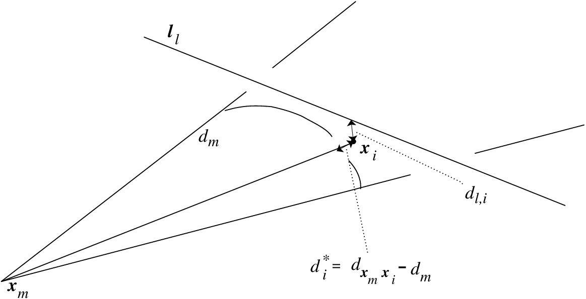
The following three situations should be treated separately:

1. 1.

   $l>i$ and $d^{*}_{i}\geq d_{l,i}$.

2. 2.

   $l<i$ and $d^{*}_{i}\geq d_{l,i}$.

3. 3.

   $d^{*}_{i}<d_{l,i}$.

In the first case, the substituted parts of the knot are at a distance $d^{*}_{i}$ which is greater than $d_{l,i}$. As a consequence, the segment $\boldsymbol{l}_{l}$ contains the point $\boldsymbol{x}_{l,i}$ which is among all points of the knot the nearest one to $\boldsymbol{x}_{i}$. Moreover, $\boldsymbol{l}_{l}$ has not yet been affected by the smoothing procedure. It is thus possible to proceed as we did for the first corner $\boldsymbol{x}_{1}$. The second case is more complicated. The point $\boldsymbol{x}_{l,i}$ on the segment $\boldsymbol{l}_{l}$ is nearer to $\boldsymbol{x}_{i}$ than any other point lying on the other segments or on the parts of the knot that have already been replaced, but the segment $\boldsymbol{l}_{l}$ has been affected by the smoothing procedure. This means that $\boldsymbol{x}_{l,i}$ could have been mapped to a new point $\boldsymbol{x}_{l,i}^{\prime}$ and it is no longer trivial to determine which is the new nearest point to $\boldsymbol{x}_{i}$. Three subcases are possible, see Fig. 9 for a visual representation:

• 2.-a)

  $\boldsymbol{x}_{l,i}$ is near the point $\boldsymbol{x}_{l-1}$ within the distance $d_{l-1}$, i. e. $\boldsymbol{x}_{l,i}$ lies on the segment $\boldsymbol{l}^{-}_{l}$. This implies that for sure $\boldsymbol{x}_{l,i}$ has been already mapped into the point $\boldsymbol{x}_{l,i}^{\prime}$ located on the arc of the smooth curve that replaced $\boldsymbol{l}_{l}^{-}$. What we know is that both segment $\boldsymbol{l}^{-}_{l}$ and the arc of the smooth curve replacing it are inside the sphere $S_{\boldsymbol{x}_{l-1}}$ of radius $d_{l-1}$. The radius $d_{i}$ of the sphere $S_{\boldsymbol{x}_{i}}$ surrounding $\boldsymbol{x}_{i}$ should be chosen in such a way that $S_{\boldsymbol{x}_{l-1}}$ and $S_{\boldsymbol{x}_{i}}$ do not penetrate into each other. We should also avoid that $S_{\boldsymbol{x}_{i}}$ penetrates inside any other sphere $S_{\boldsymbol{x}_{k}}$ with $k<i$. Due to the condition $d^{*}_{l}\geq d_{l,i}$, which is valid in this subcase, this last requirement is matched if the following inequality is satisfied:

  $$d_{i},d_{i}^{\prime}\leq d_{l,i}$$

  (47)

  Let $d_{\boldsymbol{x}_{l-1}\boldsymbol{x}_{i}}$ be the distance between $\boldsymbol{x}_{l-1}$ and $\boldsymbol{x}_{i}$. Since in our construction $d_{l-1}$ can be only less or equal to the minimal distance between $\boldsymbol{x}_{l-1}$ and any segment $\boldsymbol{l}_{n}$ with $n\neq l-1,l$, it is possible to conclude that:

  $$d_{\boldsymbol{x}_{l-1}\boldsymbol{x}_{i}}\geq d_{l-1}$$

  (48)

  If $d_{l-1}$ is strictly smaller than $d_{\boldsymbol{x}_{l-1}\boldsymbol{x}_{i}}$, then the following inequalities hold:

  $$0<d_{\boldsymbol{x}_{l-1}\boldsymbol{x}_{i}}-d_{l-1}<d_{l,i}$$

  (49)

  The left inequality is a trivial consequence of our settings. To prove that $d_{\boldsymbol{x}_{l-1}\boldsymbol{x}_{i}}-d_{l-1}<d_{l,i}$, we remember that, under the present assumptions:

  $$0<d_{\boldsymbol{x}_{l,i}\boldsymbol{x}_{l-1}}<d_{l-1}$$

  (50)

  where $d_{\boldsymbol{x}_{l,i}\boldsymbol{x}_{l-1}}$ denotes the distance between the points $\boldsymbol{x}_{l,i}$ and $\boldsymbol{x}_{l-1}$. Eq. (50) simply states the fact that the point $\boldsymbol{x}_{l,i}$ lies in the subsegment $\boldsymbol{l}_{l}^{-}$ whose length is $d_{l-1}$. Moreover, using the properties of the norm expressing the distances on Euclidean spaces, it turns out that

  $$d_{\boldsymbol{x}_{l-1}\boldsymbol{x}_{i}}\leq d_{\boldsymbol{x}_{l,i}\boldsymbol{x}_{l-1}}+d_{l,i}$$

  (51)

  Applying the second inequality appearing in Eq. (50) to (51), we obtain that $d_{\boldsymbol{x}_{l-1}\boldsymbol{x}_{i}}-d_{l-1}<d_{l,i}$, thus proving Eq. (49). As a consequence, a sphere $S_{\boldsymbol{x}_{i}}$ of radius $d_{\boldsymbol{x}_{l-1}\boldsymbol{x}_{i}}-d_{l-1}$ around the point $\boldsymbol{x}_{i}$ will never contain any point of the knot apart from the points belonging to the segments $\boldsymbol{l}_{i}$ and $\boldsymbol{l}_{i+1}$. This is due to Eq. (49), which states that the radius of $S_{\boldsymbol{x}_{i}}$ is smaller than the distance $d_{l,i}$ between $\boldsymbol{x}_{i}$ and the nearest point to $\boldsymbol{x}_{i}$. Thus, the condition (47), which is sufficient to avoid points of contacts between $S_{\boldsymbol{x}_{i}}$ and the spheres $S_{\boldsymbol{x}_{k}}$ of radii $d_{k}$ for $k=1,\ldots,i-1$ and $k\neq l-1$, is fulfilled. Moreover, when $k=l-1$, by construction the sphere $S_{\boldsymbol{x}_{l-1}}$ has only one point of contact with $S_{\boldsymbol{x}_{i}}$, see Fig. 9. Thus, it is possible to safely choose $d_{i}$ and $d_{i}^{\prime}$ as follows:

  $$d_{i}=d_{i}^{\prime}=\min\left\{d_{\boldsymbol{x}_{l-1}\boldsymbol{x}_{i}}-d_{l-1},\min\left\{\frac{l_{i}}{2},\frac{l_{i+1}}{2}\right\}\right\}$$

  (52)

  With this choice, in fact, no dangerous crossing of lines may occur between the arcs of curves already replaced and the subsegments that have still to be treated, see also Fig. 9 for a visual representation of the situation.

  

  We are left with the particular case $d_{\boldsymbol{x}_{l-1}\boldsymbol{x}_{i}}=d_{l-1}$, which can never happen under the present hypothesis that $l<i$ and $d^{*}_{i}\geq d_{l,i}$. As a matter of fact, if $d_{\boldsymbol{x}_{l-1}\boldsymbol{x}_{i}}=d_{l-1}$, the quantity $d_{i}^{*}$ defined in Eq. (46) is zero and, as a consequence, $d_{i}^{*}<d_{l,i}$, because $d_{l,i}$ can never vanish since the segments $\boldsymbol{l}_{l}$ and $\boldsymbol{l}_{i}$ are not allowed to intersect. The situations in which $d_{i}^{*}=0$ will be treated in the next point dedicated to case 3 of page IV.

• 2.-b)

  $\boldsymbol{x}_{l,i}$ is near the point $\boldsymbol{x}_{l}$ within a distance which is less than $d_{l}$, i. e. it lies on the segment $\boldsymbol{l}_{l}^{+}$ that has already been substituted. In that case the procedure to determine $d_{i},d_{i}^{\prime}$ is analogous to that used in the case 2.-a).

• 2.-c)

  $\boldsymbol{x}_{l,i}$ is on the subsegment $\boldsymbol{l}_{l}^{0}$, In that case there is no problem because this subsegment has not been replaced with an arc of a curve and we may proceed by taking:

  $$d_{i}=d_{i}^{\prime}=\min\left\{d_{l,i},\min\left\{\frac{l_{i}}{2},\frac{l_{i+1}}{2}\right\}\right\}$$

  (53)

Finally, we deal with the case 3 of page IV. We distinguish the following two subcases:

• 3-a)

  $d_{i}^{*}>0$. In this case we choose the radius of the sphere $S_{\boldsymbol{x}_{i}}$ around the point $\boldsymbol{x}_{i}$ to be equal to $d_{i}^{*}$, i. e.:

  $$d_{i}=d_{i}^{\prime}=\min\left\{d_{i}^{*},\min\left\{\frac{l_{i}}{2},\frac{l_{i+1}}{2}\right\}\right\}$$

  (54)

• 3-b)

  $d_{i}^{*}=0$. As a consequence, there exist a sphere $S_{\boldsymbol{x}_{m}}$ of radius $d_{m}$ centered at the point $\boldsymbol{x}_{m}$ for some value of $m\leq i-1$ such that $\boldsymbol{x}_{i}$ lies on the border of this sphere. On the other side, no point of the knot may be nearer to $\boldsymbol{x}_{i}$ than $\boldsymbol{x}_{l,i}$, which is at the distance $d_{l,i}>d^{*}_{i}=0$ from $\boldsymbol{x}_{i}$. Yet, it may happen that there exists another sphere, let say $S_{\boldsymbol{x}_{n}}$, with $n\leq i-1$ and $n\neq m$ centered at a point $\boldsymbol{x}_{n}$, such that the distance between the border of $S_{\boldsymbol{x}_{n}}$ and $\boldsymbol{x}_{i}$ is less than $d_{l,i}$. To take into account this case, it is useful to compute also the quantity $d_{i}^{*\prime}$³³ 3 We do not discuss here the particular case in which $d_{i}^{*\prime}$ is also equal to zero, which can be easily treated.:

  $$d^{*\prime}_{i}=\min_{\begin{subarray}{c}k=1,\ldots,i-1\\ k\neq m\end{subarray}}\left\{d_{l,i},d_{\boldsymbol{x}_{k}\boldsymbol{x}_{i}}-d_{k}\right\}$$

  (55)

  At this point a possible way to define $d_{i}$ and $d_{i}^{\prime}$ consists in putting

  $$d_{i}=d_{i}^{\prime}=\min\left\{\min\left\{d_{i}^{*\prime},\frac{d_{k}}{2}\right\},\min\left\{\frac{l_{i}}{2},\frac{l_{i+1}}{2}\right\}\right\}$$

  (56)

  and to decrease the value of the radius of the sphere $S_{\boldsymbol{x}_{k}}$ as follows:

  $$d_{k}\longrightarrow\frac{d_{k}}{2}$$

  (57)

  Clearly, the choice of $d_{i},d_{i}^{\prime}$ given above does not allow crossings of the lines that can change the type of the knot.

Let us stress that, within the procedure illustrated above, at each stage $i$ the arcs of the curves replacing the corners are always contained inside a sphere centered at the $i-$th corner. The spheres corresponding to different corners never intersect themselves apart from one point on their surfaces which may be in common. In this way, there is no possibility that the trajectory of the knot crosses itself during the replacement of the sharp corners causing unwanted changes of the topology of the knot. The result is that the trajectory of the discrete knot becomes a $G^{1}-$curve, which is the condition sufficient in order to compute the Vassiliev knot invariant of degree 2 without the systematic errors related to the presence of the sharp corners. The only drawback is that the parameters $d_{i}$, and thus the portions of the corners that have been replaced, become smaller and smaller when the value of $i$ increases. This is a drawback because an extensive Monte Carlo sampling procedure is required in order to evaluate $\varrho(C)$ with a good approximation if the arcs of curves replacing the corners exhibit sharp turns.

References

- [1] Wasserman, S. A., Cozzarelli, N. R.: Biochemical topology: applications to DNA recombination and replication. Science 232, 951-960 (1986)
- [2] Delbruck, M.: Mathematical Problems in the Biological Sciences. Proc. Symp. Appl. Marh. 14, Providence, RI: American Mathematical Society, 55 (1962)
- [3] Bowick, M. J., Chander, L., Schiff, E. A., Srivastava, A. M.: The Cosmological Kibble Mechanism in the Laboratory: String Formation in Liquid Crystals. Science 263, 943-945 (1994)
- [4] Bäuerle, C., Bunkov, Yu. M., Fisher, S. N., Godfrin, H., Pickett, G. R.: Laboratory simulation of cosmic string formation in the early Universe using superfluid 3He. Nature 382, 332-334 (1996); Ruutu, V. M. H., Eltsov, V. B., Gill, A. J., Kibble, T. W. B., Krusius, M., Makhlin, Yu. G., Plaçais, B., Volovik, G. E., Xu, W.: Vortex formation in neutron-irradiated superfluid 3He as an analogue of cosmological defect formation. Nature 382, 334-336 (1996)
- [5] Araki, T., Tanaka, H.: Colloidal Aggregation in a Nematic Liquid Crystal: Topological Arrest of Particles by a Single-Stroke Disclination Line. Phys. Rev. Lett. 97, 127801-4 (2006); Tkalec, U., Ravnik, M., Čopar, S., Žumer, S., Muševič, I. : Reconfigurable Knots and Links in Chiral Nematic Colloids. Science 333, 62-65 (2011); Žumer, S.: 21st International Liquid Crystal Conference, Keystone, Colorado, USA, July 2–7, 2006, Kinsley & Associates, Littletown, (2006)
- [6] Alexander, J. W.: Topological Invariants of Knots and Links. Trans. Amer. Math. Soc. 30, 275-306 (1928)
- [7] Freyd, P., Yetter, D., Hoste, J., Lickorish, W. B. R., Millet, K., Ocneanu, A.: A new polynomial invariant of knots and links. Bull. AMS 12, 239-246 (1985)
- [8] Kontsevich, M.: Vassiliev’s knot invariants, Preprint, Max-Planck-Institut für Mathematik, Bonn; Bar-Natan, D.: On the Vassiliev knot invariants, Harvard preprint (1992); Bar-Natan, D.: On the Vassiliev Knot Invariants, Topology 34, 423-472 (1995)
- [9] Labastida, J. M. F., Ramallo, A. V.: Operator formalism for Chern-Simons theories. Phys. Lett. B 227, 92-102 (1989)
- [10] Guadagnini, E., Martellini, M., Mintchev, M.: Braids and quantum group symmetry in Chern-Simons theory. Nucl. Phys. B 336, 581-609 (1990)
- [11] Vologodskii, A. V., Lukashin, A. V., Frank-Kamenetskii, M. D., Anshelevich, V. V.: The knot problem in statistical mechanics of polymer chains. Zh. Eksp. Teor. Fiz. 66, 2153-2163 (1974)
- [12] Nonweiler T. T. F.: The Numerical Evaluation of Curvilinear Integrals and Areas Defined by Discrete Data. Inter-university/research councils series (1972)
- [13] Davis, P. and Rabinowitz, P.: Methods of Numerical Integration. 2nd Ed, New York, Academic Press (1984)
- [14] Atkinson, K. and Venturino, E.: Numerical Evaluation of Line Integrals. Siam J. Numer. Anal. 30, 882-888 (1993)
- [15] Knott, G. D.: Interpolating Cubic Splines. Boston, Birkhäuser (2000)
- [16] Dunin-Barkowski, P., Sleptsov, A., Smirnov, A.: Kontsevich integral for knots and Vassiliev invariants. Int. J. Mod. Phys. A 28, 1330025-62 (2013)
- [17] Zhao, Y., Ferrari, F.: A study of polymer knots using a simple knot invariant consisting of multiple contour integrals. JSTAT 2013, P10010 (2013)
- [18] Davis, P. J., Rabinowitz, P.: Methods of numerical integration. Boston, MA, Academic Press, 1984
- [19] Madras, N., Orlitsky, A., Sepp, L. A.: Monte Carlo Generation of Self-Avoiding Walks with Fixed Endpoints and Fixed Length. J. Stat. Phys. 38, 159-183 (1990)
- [20] Lesh, N., Mitzenmacher, M., Whitesides, S.: A Complete and Effective Move Set for Simplified Protein Folding. Proceedings of the Seventh Annual International Conference on Research in Computational Molecular Biology (RECOMB’03), 188-195 (2003)
- [21] Aragao de Carvalho, C., Caracciolo, S., Fröhlich, J.: Polymers and theory in four dimensions. Nucl. Phys. B 215, 209-248 (1983); Berg, B., Foerster, D.: Random paths and random surfaces on a digital computer. Phys. Lett. B 106, 323-326 (1981)
- [22] Witten, E.: Quantum field theory and the Jones polynomial. Commun. Math. Phys. 121, 351-399 (1989)
- [23] Cattaneo, A. S., Cotta-Ramusino, P., Martellini, M.: Three-dimensional BF theories and the Alexander-Conway invariant of knots. Nucl. Phys. B 436(1-2), 355-382 (1995)
- [24] Polyak, M., Viro, O.: On the Casson knot invariant, J. Knot Theory Ramifications 10, 711-738 (2001)
- [25] Qu, L. and He, D.: Solving Numerical Integration by Particle Swarm Optimization. Work published in the Proceedings of ICICA 2010, Part II, Zhu, R. et Al. (Eds), Berlin, Heidelberg, Springer Verlag, 228-235 (2010)
- [26] Koniaris, K., Muthukumar, M.: Knottedness in ring polymers. Phys. Rev. Lett. 66, 2211-2214 (1991)
- [27] Taylor, W. R., Aszódi, A.: Protein Geometry, Classification, Topology and Symmetry: A Computational Analysis of Structure. New York, Taylor & Francis Group, (2005)
- [28] He, Y., Gu X. F., Qin H.: Automatic Shape Control of Triangular B-Splines of Arbitrary Topology. Jour. Comput. Sci. & Technol. 21, 232-237 (2006)