The enriched Crouzeix–Raviart elements are equivalent to the Raviart–Thomas elementsThanks: The first author was supported by the NSFC Project 11271035 and by the NSFC Key Project 11031006.

Jun Hu^∗ Address: ^∗ LMAM and School of Mathematical Sciences, Peking University, Beijing 100871, P. R. China Email address: hujun@math.pku.edu.cn and Rui Ma^† Address: ^† LMAM and School of Mathematical Sciences, Peking University, Beijing 100871, P. R. China Email address: maruipku@gmail.com

Abstract.

For both the Poisson model problem and the Stokes problem in any dimension, this paper proves that the enriched Crouzeix–Raviart elements are actually identical to the first order Raviart–Thomas elements in the sense that they produce the same discrete stresses. This result improves the previous result in literature which, for two dimensions, states that the piecewise constant projection of the stress by the first order Raviart–Thomas element is equal to that by the Crouzeix–Raviart element. For the eigenvalue problem of Laplace operator, this paper proves that the error of the enriched Crouzeix–Raviart element is equivalent to that of the Raviart–Thomas element up to higher order terms.

Key words and phrases:

Crouzeix–Raviart element, Enriched Crouzeix–Raviart element, Raviart–Thomas element, the Poisson equation, the Stokes equation, eigenvalue problem.
AMS Subject Classification: 65N30, 65N15, 35J25

1. introduction

The aim of this paper is to prove the enriched Crouzeix–Raviart (ECR hereafter) elements by Hu, Huang and Lin [21] are equivalent to the first order Raviart–Thomas elements (RT hereafter). The first main result proves that ECR elements are identical to RT elements for both the Poisson and Stokes problems in any dimension. More precisely, for the Poisson problem imposed a piecewise constant right–hand function $f$ , it is proved that

(1.1)

\sigma_{\rm RT}=\nabla_{\rm NC}u_{\rm ECR}\text{ and }u_{\rm RT}=\Pi_{0}u_{\rm ECR},

where $u_{\rm ECR}$ and $(\sigma_{\rm RT},u_{\rm RT})$ denote the finite element solutions by the ECR and RT elements, respectively; while for the Stokes problem imposed a piecewise constant right–hand function $\bm{f}$ , it is established that

(1.2)

\bm{\sigma}_{\rm RT}=\nabla_{\rm NC}\bm{u}_{\rm ECR}+p_{\rm ECR}\id\text{ and }\bm{u}_{\rm RT}=\Pi_{0}\bm{u}_{\rm ECR}+\mathcal{L}u_{\rm ECR},

where $(\bm{u}_{\rm ECR},p_{\rm ECR})$ and $(\bm{\sigma}_{\rm RT},\bm{u}_{\rm RT})$ denote the finite element solutions by the ECR and RT elements, respectively. Herein and throughout this paper, $\Pi_{0}$ denotes the piecewise constant $L^{2}$ projection with respect to a shape–regular partition $\mathcal{T}$ of $\Omega$ consisting of $n$ -simplices, and $\mathcal{L}$ is some linear operator. The second main result proves that for the eigenvalue problem of Laplace operator

(1.3)

\|\nabla_{\rm NC}(u-u_{\rm ECR})\|=\|\nabla u-\sigma_{\rm RT}\|+h.o.t.

where the constants involved in the high order term depend on the corresponding eigenvalue. Throughout this paper, $\|v\|$ denotes $(v,v)^{1/2}_{L^{2}(\Omega)}$ , for any $v\in L^{2}(\Omega)$ . See the next two sections for more details of the notations.

The history perspective justifies the novelty of both (1.1) and (1.2). For general right–hand function $f$

(1.4)

\|\nabla_{\rm NC}(u-u_{ECR})\|=\|\nabla u-\sigma_{\rm RT}\|

hold up to data oscillation. Indeed, it is the first time that the RT elements are proved in such a direct and simple way to be identical to nonconforming finite elements in any dimension while the previous results state some relations between the two dimensional Crouzeix–Raviart (CR hereafter) and RT elements; see below and also [3, 11, 26] for more details. These results imply that the RT element can not be equivalent to the CR element in general, which gives a negative answer to an open problem in [15].

The study on the relations between nonconforming finite elements and mixed finite elements can date back to the pioneer and remarkable work by Arnold and Brezzi in 1985 [3]. In particular, for the two dimensional biharmonic equation, it was proved that the first order Hellan–Herrmann–Johnson element [19, 20, 25] is identical to the modified Morley element which differs from the usual Morley element [29] only by presence of the interpolation operator in the right–hand side; while for the two dimensional Poisson problem, it was shown that the $L^{2}$ projection onto the first order RT element space of the stress by the CR element, enriched by piecewise cubic bubbles, is identical to the stress by the RT element. By proposing initially a projection finite element method, Arbogast and Chen [1] generalized successfully the idea of [3] to most mixed methods of more general second order elliptic problems in both two and three dimensions. In particular, they showed that most mixed methods can be implemented by solving projected nonconforming methods with symmetric positive definite stiff matrixes, and that stresses by mixed methods are $L^{2}$ projections of those by nonconforming methods. Let $\sigma_{\rm RT}$ be the discrete stress by the RT element, and $u_{\rm CR}$ be the displacement by the CR element of the two dimensional Poisson equation. Suppose that $f$ is a piecewise constant function with respect to $\mathcal{T}$ . Marini further explored the relation between the RT and CR elements of [3] to derive the following relation [26]:

(1.5)

\sigma_{\rm RT}|_{K}=\nabla u_{\rm CR}|_{K}-\frac{f_{K}}{2}(x-{\rm mid}(K))\quad x\in K\text{ for any }K\in\mathcal{T},

where $f_{K}:=f|_{K}$ denotes the restriction on $K$ of $f$ and ${\rm mid}(K)$ denotes the centroid of $K$ . This important identity was exploited by Brenner [8] to design an optimal multigrid method for the RT element, and by Carstensen and Hoppe to establish, for the first time, quasi–orthogonality and consequently convergence of both the adaptive RT and CR elements in [13] and [12], respectively. For the two dimensional Stokes equation, a similar identity was first accomplished in [11]:

(1.6)

\begin{split}&\bm{\sigma}_{\rm RT}|_{K}=\nabla\bm{u}_{\rm CR}-\frac{\bm{f}_{K}}{2}\otimes(x-{\rm mid}(K))+p_{\rm CR}|_{K}\id,\\ &\bm{u}_{\rm RT}|_{K}=\Pi_{0}\bm{u}_{\rm CR}+\frac{1}{4}\Pi_{0}(\dev(\bm{f}_{K}\otimes(x-{\rm mid}(K))))(x-{\rm mid}(K)),\end{split}

$x\in K$ for any $K\in\mathcal{T}$ . Here $(\bm{u}_{\rm CR},p_{\rm CR})$ and $(\bm{\sigma}_{\rm RT},\bm{u}_{\rm RT})$ are finite element solutions by the CR and RT elements, respectively, and $\bm{f}_{K}$ is the restriction on $K$ of the piecewise constant function $\bm{f}$ . Given two vectors $a\in\mathbb{R}^{2}$ and $b\in\mathbb{R}^{2}$ , $a\otimes b:=ab^{T}$ defines a $2\times 2$ matrix of rank one. See also [24] for a similar relation between the CR and RT elements for the two dimensional Stokes–like problems. Such a beautiful identity is also used to prove convergence and optimality of the adaptive pseudostress method in [11].

There is another direction for the study on the relations between nonconforming finite elements and mixed finite elements, which may start with the remarkable work by Braess [6]. A recent paper on the two dimensional Poisson model problem due to Carstensen, Peterseim, and Schedensack [15] states more general and profound comparison results of mixed, nonconforming and conforming finite element methods

(1.7)

\|\nabla u-\sigma_{\rm RT}\|\leq C\|\nabla_{\rm NC}(u-u_{\rm CR})\|\approx\|\nabla(u-u_{\rm C})\|,

hold up to data oscillation and up to mesh-size independent generic multiplicative constants, where $C$ is a generic constant independent of the meshsize, and $u_{\rm C}$ is the finite element solution by the conforming Courant element. See [18, 27] for some relevant results in this direction. By a numerical counterexample, it was also demonstrated in [15] that the converse estimate

(1.8)

\|\nabla_{\rm NC}(u-u_{\rm CR})\|\leq C\|\nabla u-\sigma_{\rm RT}\|

does not hold. In Subsection 3.3, we give an example where the right hand side of the above inequality vanishes while the left hand side is nonzero, which implies that the converse of (1.8) is not valid.

This paper is organised as follows. Section 2 presents the Poisson equation, Stokes equation and their mixed formulations. This section also introduces the ECR and RT elements. Section 3 proves the equivalence between the ECR and RT elements for the Poisson equation and Stokes equation respectively. Section 4 proves the equivalence between the ECR and RT elements for the eigenvalue problem of Laplace operator. Section 5 shows some numerical results by ECR elements. In the end, the appendix presents the basis functions and convergence analysis of ECR elements.

2. Poisson equation, stokes equation and nonconforming finite element methods

We present the Poisson equation, stokes equation and their nonconforming finite element methods in this section. Throughout this paper, let $\Omega\subset\mathbb{R}^{n}$ denote a bounded domain, which, for the sake of simplicity, we suppose to be a polytope.

2.1. The Poisson equation

Given $f\in L^{2}(\Omega,\mathbb{R})$ , the Poisson model problem finds $u\in H^{1}_{0}(\Omega,\mathbb{R})$ such that

(2.1)

(\nabla u,\nabla v)=(f,v)\quad\text{ for all }v\in H^{1}_{0}(\Omega,\mathbb{R}).

By introducing an auxiliary variable $\sigma:=\nabla u$ , the problem can be formulated as the following equivalent mixed problem which seeks $(\sigma,u)\in H(\operatorname{div},\Omega,\mathbb{R}^{n})\times L^{2}(\Omega,\mathbb{R})$ such that

(2.2)

\begin{split}&(\sigma,\tau)+(u,\operatorname{div}\tau)=0\quad\text{ for any }\tau\in H(\operatorname{div},\Omega,\mathbb{R}^{n}),\\ &(\operatorname{div}\sigma,v)=(-f,v)\quad\text{ for any }v\in L^{2}(\Omega,\mathbb{R}).\end{split}

2.2. The stokes equation

Given $\bm{f}\in L^{2}(\Omega,\mathbb{R}^{n})$ , the Stokes problem models the motion of incompressible fluids occupying $\Omega$ which finds $(\bm{u},p)\in H_{0}^{1}(\Omega,\mathbb{R}^{n})\times L_{0}^{2}(\Omega,\mathbb{R}):=\{q\in L^{2}(\Omega,\mathbb{R}),\int_{\Omega}qdx=0\}$ such that

(2.3)

\begin{split}&(\nabla\bm{u},\nabla\bm{v})+(\operatorname{div}\bm{v},p)=(\bm{f},\bm{v})\quad\text{ for any }\bm{v}\in H_{0}^{1}(\Omega,\mathbb{R}^{n})\,,\\ &(\operatorname{div}\bm{u},q)=0\text{ for any }q\in L_{0}^{2}(\Omega,\mathbb{R}).\end{split}

where $\bm{u}$ and $p$ are the velocity and pressure of the flow, respectively. Given any $n\times n$ matrix–valued function $\bm{\tau}$ , its divergence $\operatorname{div}\bm{\tau}$ is defined as

\operatorname{div}\bm{\tau}:=\begin{pmatrix}\sum\limits_{j=1}^{n}\frac{\partial\tau_{1,j}}{\partial x_{j}}\\ \vdots\\ \sum\limits_{j=1}^{n}\frac{\partial\tau_{k,j}}{\partial x_{j}}\\ \vdots\\ \sum\limits_{j=1}^{n}\frac{\partial\tau_{n,j}}{\partial x_{j}}\end{pmatrix},

while its trace reads

\tr\bm{\tau}:=\sum\limits_{i=1}^{n}\tau_{ii}.

Let $\id\in\mathbb{R}^{n\times n}$ be the $n\times n$ identity matrix. This allows to define the deviatoric part of $\bm{\tau}$ as

\dev\bm{\tau}:=\bm{\tau}-1/n\ \tr(\bm{\tau})\id.

The definition of the pseudostress $\bm{\sigma}:=\nabla\bm{u}+p\id$ yields the equivalent pseudostress formulation [4, 9, 10, 11, 14, 24]: Find $(\bm{\sigma},\bm{u})\in\hat{H}(\operatorname{div},\Omega,\mathbb{R}^{n\times n})\times L^{2}(\Omega,\mathbb{R}^{n})$ such that

(2.4)

\begin{split}&(\dev\bm{\sigma},\dev\bm{\tau})+(\bm{u},\operatorname{div}\bm{\tau})=0\quad\text{ for any }\bm{\tau}\in\hat{H}(\operatorname{div},\Omega,\mathbb{R}^{n\times n})\,,\\ &(\operatorname{div}\bm{\sigma},\bm{v})=-(\bm{f},\bm{v})\text{ for any }\bm{v}\in L^{2}(\Omega,\mathbb{R}^{n}).\end{split}

Herein and throughout this paper, the space $\hat{H}(\operatorname{div},\Omega,\mathbb{R}^{n\times n})$ is defined as

\hat{H}(\operatorname{div},\Omega,\mathbb{R}^{n\times n}):=\{\bm{\tau}\in H(\operatorname{div},\Omega,\mathbb{R}^{n\times n}):\int_{\Omega}\tr\bm{\tau}dx=0\}.

2.3. Triangulations

The simplest nonconforming finite elements for both Problem (2.1) and Problem (2.3) are the CR elements proposed in [16] while the simplest mixed finite elements for Problem (2.2) and Problem (2.4) are the first order RT element due to [30] and [4, 9, 10, 11, 14, 24], respectively. Suppose that $\overline{\Omega}$ is covered exactly by shape–regular partitions $\mathcal{T}$ consisting of $n$ -simplices in $n$ dimensions. Let $\mathcal{E}$ denote the set of all $n-1$ dimensional subsimplices of $\mathcal{T}$ , and $\mathcal{E}(\Omega)$ denote the set of all the $n-1$ dimensional interior subsimplices, and $\mathcal{E}(\partial\Omega)$ denote the set of all the $n-1$ dimensional boundary subsimplices. Given $E\in\mathcal{E}$ , let $\nu_{E}$ be unit normal vector and $[\cdot]$ be jumps of piecewise functions over $E$ , namely

[v]:=v|_{K^{+}}-v|_{K^{-}}

for piecewise functions $v$ and any two elements $K^{+}$ and $K^{-}$ which share the common sub-simplice $E$ . Note that $[\cdot]$ becomes traces of functions on $E$ for boundary sub-simplices $E$ .

2.4. The enriched Crouzeix–Raviart elements for both the Poisson and Stokes equations

Given $\omega\subset\Omega$ and an integer $m\geq 0$ , let $P_{m}(\omega)$ denote the space of polynomials of degree $\leq m$ over $\omega$ . The Crouzeix-Raviart element space $V_{\rm CR}$ over $\mathcal{T}$ is defined as

V_{\rm CR}:=\begin{array}[t]{l}\big\{v\in L^{2}(\Omega,\mathbb{R}):v|_{K}\in P_{1}(K)\text{ for each }K\in\mathcal{T},\int_{E}[v]dE=0,\\ \text{ for all }E\in\mathcal{E}(\Omega)\,,\text{ and }\int_{E}vdE=0\text{ for all $E\in\mathcal{E}(\partial\Omega)$ }\big\}\,.\end{array}

To obtain a nonconforming finite element method that is able to produce lower bounds of eigenvalues of second order elliptic operators, it was proposed in [21] to enrich the shape function space $P_{1}(K)$ by $\sspan\{\sum\limits_{i=1}^{n}x_{i}^{2}\}$ on each element. This leads to the following shape function space

(2.5)

{\rm ECR}(K):=P_{1}(K)+\sspan\Big\{\sum\limits_{i=1}^{n}x_{i}^{2}\Big\}\quad\text{ for any }K\in\mathcal{T}.

The enriched Crouzeix-Raviart element space $V_{\rm ECR}$ is then defined by

V_{\rm ECR}:=\begin{array}[t]{l}\big\{v\in L^{2}(\Omega,\mathbb{R}):v|_{K}\in{\rm ECR}(K)\text{ for each }K\in\mathcal{T},\int_{E}[v]dE=0,\\ \text{ for all }E\in\mathcal{E}(\Omega)\,,\text{ and }\int_{E}vdE=0\text{ for all $E\in\mathcal{E}(\partial\Omega)$ }\big\}\,.\end{array}

The enriched Crouzeix–Raviart element method of Problem (2.1) finds $u_{\rm ECR}\in V_{\rm ECR}$ such that

(2.6)

(\nabla_{\rm NC}u_{\rm ECR},\nabla_{\rm NC}v)=(f,v)\text{ for all }v\in V_{\rm ECR}.

In order to construct a stable finite element method for the Stokes problem, we propose the following finite element space for the pressure

(2.7)

Q_{\rm ECR}:=\{q\in L^{2}_{0}(\Omega,\mathbb{R}),q|_{K}\in P_{0}(K)\text{ for each }K\in\mathcal{T}\}.

The enriched Crouzeix–Raviart element method of Problem (2.3) seeks $(\bm{u}_{\rm ECR},p_{\rm ECR})\in(V_{\rm ECR})^{n}\times Q_{\rm ECR}$ such that

(2.8)

\begin{split}&(\nabla_{\rm NC}\bm{u}_{\rm ECR},\nabla_{\rm NC}\bm{v})+(\operatorname{div}_{\rm NC}\bm{v},p_{\rm ECR})=(\bm{f},\bm{v})\quad\text{ for any }\bm{v}\in(V_{\rm ECR})^{n}\,,\\ &(\operatorname{div}_{\rm NC}\bm{u}_{\rm ECR},q)=0\text{ for any }q\in Q_{\rm ECR}.\end{split}

Since $V_{\rm CR}\subset V_{\rm ECR}$ , the well-posedness of Problem (2.8) follows immediately from that for the Crouzeix–Raviart element method of Problem (2.3), see [16] for more details.

2.5. The Raviart–Thomas elements for both the Poisson and Stokes equations

For the Poisson equation, one famous mixed finite element is the first order Raviart–Thomas element whose shape function space is

{\rm RT}(K):=(P_{0}(K))^{n}+xP_{0}(K)\text{ for any }K\in\mathcal{T}.

Then the corresponding global finite element space reads

(2.9)

{\rm RT}(\mathcal{T}):=\{\tau\in H(\operatorname{div},\Omega,\mathbb{R}^{n}):\tau|_{K}\in{\rm RT}(K)\text{ for any }K\in\mathcal{T}\}.

To get a stable pair of space, the piecewise constant space is proposed to approximate the displacement, namely,

(2.10)

U_{\rm RT}:=\{v\in L^{2}(\Omega,\mathbb{R}):v|_{K}\in P_{0}(K)\text{ for any }K\in\mathcal{T}\}.

The Raviart–Thomas element method of Problem (2.2) seeks $(\sigma_{\rm RT},u_{\rm RT})\in{\rm RT}(\mathcal{T})\times U_{\rm RT}$ such that

(2.11)

\begin{split}&(\sigma_{\rm RT},\tau)+(u_{\rm RT},\operatorname{div}\tau)=0\quad\text{ for any }\tau\in{\rm RT}(\mathcal{T}),\\ &(\operatorname{div}\sigma_{\rm RT},v)=(-f,v)\quad\text{ for any }v\in U_{\rm RT}.\end{split}

Define

(2.12)

(\widehat{{\rm RT}}(\mathcal{T}))^{n}:=({\rm RT}(\mathcal{T}))^{n}\cap\hat{H}(\operatorname{div},\Omega,\mathbb{R}^{n\times n}).

The Raviart–Thomas element method of Problem (2.4) searches for $(\bm{\sigma}_{\rm RT},\bm{u}_{\rm RT})\in(\widehat{{\rm RT}}(\mathcal{T}))^{n}\times(U_{\rm RT})^{n}$ such that

(2.13)

\begin{split}&(\dev\bm{\sigma}_{\rm RT},\dev\bm{\tau})+(\bm{u}_{\rm RT},\operatorname{div}\bm{\tau})=0\quad\text{ for any }\bm{\tau}\in(\widehat{{\rm RT}}(\mathcal{T}))^{n}\,,\\ &(\operatorname{div}\bm{\sigma}_{\rm RT},\bm{v})=-(\bm{f},\bm{v})\text{ for any }\bm{v}\in(U_{\rm RT})^{n}.\end{split}

3. Equivalence between the ECR and RT elements

In this section we assume that both $f$ and $\bm{f}$ are piecewise constant with respect to $\mathcal{T}$ .

3.1. Equivalence between the ECR and RT elements for the Poisson equation

Given any $K\in\mathcal{T}$ , let $E_{i}\,,i=1,2,\cdots,n+1$ , be its $n-1$ dimensional sub-simplices. Let $\phi_{i},i=1,2,\cdots,n+1$ , and $\phi_{K}$ be basis functions of the shape function space ${\rm ECR}(K)$ , so that

(3.1)

\begin{split}&\int_{E_{i}}\phi_{j}dE=\delta_{i,j}:=\left\{\begin{array}[]{ll}1&\text{ if }i=j\\ 0&\text{ otherwise}\end{array}\right.,\text{ and }\int_{K}\phi_{j}dx=0,i,j=1,\cdots,n+1,\\ &\int_{K}\phi_{K}dx=1,\text{ and }\int_{E_{i}}\phi_{K}dE=0,i=1,\cdots,n+1.\end{split}

See the appendix for the specific expressions.

Lemma 3.1.

Let $u_{\rm ECR}$ be the solution of Problem (2.6). There holds that

\nabla_{\rm NC}u_{\rm ECR}\in H(\operatorname{div},\Omega,\mathbb{R}^{n}).

Remark 3.2.

Since $u_{\rm ECR}$ is nonconforming in the sense that $u_{\rm ECR}\not\in H^{1}(\Omega,\mathbb{R})$ , it is remarkable that $\nabla_{\rm NC}u_{\rm ECR}$ is $H(\operatorname{div})$ conforming.

Proof.

Let $(\sigma_{\rm RT},u_{\rm RT})$ the solution of Problem (2.11). Since $\sigma_{\rm RT}\cdot\nu_{E}$ are a constant and $\int_{E}[v]dE=0$ for any $E\in\mathcal{E}$ and $v\in V_{\rm ECR}$ , an integration by parts plus the second equation of (2.11) yield

(\sigma_{\rm RT},\nabla_{\rm NC}v)=\sum\limits_{E\in\mathcal{E}}\int_{E}\sigma_{\rm RT}\cdot\nu_{E}vdE-(\operatorname{div}\sigma_{\rm RT},v)=(f,v).

This and (2.6) lead to

(3.2)

(\nabla_{\rm NC}u_{\rm ECR}-\sigma_{\rm RT},\nabla_{\rm NC}v)=0\quad\text{for any }v\in V_{\rm ECR}.

Given $E\in\mathcal{E}(\Omega)$ , let $v_{E}\in V_{ECR}$ such that

\int_{E}v_{E}dE=1,\int_{E^{\prime}}v_{E}dE=0\text{ for any }E^{\prime}\text{ other than }E,\text{ and }\int_{K}vdx=0\text{ for all }K\in\mathcal{T}.

Since $x\cdot\nu_{E}$ is a constant on $E$ , $\nabla_{\rm NC}u_{\rm ECR}\cdot\nu_{E}$ is a constant on $E$ . Since $\operatorname{div}_{\rm NC}(\nabla_{\rm NC}u_{\rm ECR}-\sigma_{\rm RT})$ is a piecewise constant function, since both the average $\big\{(\nabla_{\rm NC}u_{\rm ECR}-\sigma_{\rm RT})\big\}\cdot\nu_{E}$ and the jump $[(\nabla_{\rm NC}u_{\rm ECR}-\sigma_{\rm RT})]\cdot\nu_{E}$ are a constant on $E$ , an integration by parts derives

\begin{split}0&=(\nabla_{\rm NC}u_{\rm ECR}-\sigma_{\rm RT},\nabla_{\rm NC}v_{E})\\ &=[(\nabla_{\rm NC}u_{\rm ECR}-\sigma_{\rm RT})]\cdot\nu_{E}\int_{E}v_{E}dE+\big\{(\nabla_{\rm NC}u_{\rm NC}-\sigma_{\rm RT})\big\}\cdot\nu_{E}\int_{E}[v_{E}]dE\\ &=[(\nabla_{\rm NC}u_{\rm ECR}-\sigma_{\rm RT})]\cdot\nu_{E}.\end{split}

Hence $\nabla_{\rm NC}u_{\rm ECR}\in H(\operatorname{div},\Omega,\mathbb{R}^{n})$ , which completes the proof. ∎

Theorem 3.3.

Let $u_{\rm ECR}$ and $(\sigma_{\rm RT},u_{\rm RT})$ be the solutions of problems (2.6) and (2.11), respectively. Then there holds

\sigma_{\rm RT}=\nabla_{\rm NC}u_{\rm ECR}\text{ and }u_{\rm RT}=\Pi_{0}u_{\rm ECR},

where $\Pi_{0}$ is the piecewise constant $L^{2}$ projection operator.

Proof.

By Lemma 3.1, we only need to prove that $(\nabla_{\rm NC}u_{\rm ECR},\Pi_{0}u_{\rm ECR})$ is the solution of Problem (2.11). In fact, given any $\tau\in{\rm RT}(\mathcal{T})$ , an integration by parts yields

(\nabla_{\rm NC}u_{\rm ECR},\tau)=-(u_{\rm ECR},\operatorname{div}\tau)+\sum\limits_{E\in\mathcal{E}}\int_{E}[u_{\rm ECR}]\tau\cdot\nu_{E}dE=-(u_{\rm ECR},\operatorname{div}\tau).

Hence

(\nabla_{\rm NC}u_{\rm ECR},\tau)+(\Pi_{0}u_{\rm ECR},\operatorname{div}\tau)=0,

which is the first equation of Problem (2.11). To prove the second equation of Problem (2.11), given any $K$ , let $v=\phi_{K}$ in (2.6), an integration by parts leads to

(f,\phi_{K})=(\nabla_{\rm NC}u_{\rm ECR},\nabla_{\rm NC}\phi_{K})=-(\operatorname{div}\nabla_{\rm NC}u_{\rm ECR},\phi_{K})+\sum\limits_{E\subset\partial K}\int_{E}\nabla_{\rm NC}u_{\rm ECR}\cdot\nu_{E}\phi_{K}dE.

Since $\nabla_{\rm NC}u_{\rm ECR}\cdot\nu_{E}$ is a constant on $E$ and $\int_{E}\phi_{K}dE=0$ , this yields

\operatorname{div}\nabla_{\rm NC}u_{\rm ECR}(1,\phi_{K})=-f_{K}(1,\phi_{K})\Rightarrow\operatorname{div}\nabla_{\rm NC}u_{\rm ECR}=-f_{K},

which completes the proof. ∎

3.2. Equivalence between the ECR and RT elements for the Stokes equation

Lemma 3.4.

Let $(\bm{u}_{\rm ECR},p_{\rm ECR})$ be the solution of Problem (2.8). There holds that

\nabla_{\rm NC}\bm{u}_{\rm ECR}+p_{\rm ECR}\id\in H(\operatorname{div},\Omega,\mathbb{R}^{n\times n}).

Proof.

The proof is actually similar to that of Lemma 3.1. Let $(\bm{\sigma}_{\rm RT},\bm{u}_{\rm RT})$ be the solution of Problem (2.13). Given any $\bm{v}\in(V_{ECR})^{n}$ , it follows from an integration by parts and the second equation of Problem (2.13) that

(\bm{\sigma}_{\rm RT},\nabla_{\rm NC}\bm{v})=(\bm{f},\bm{v})+\sum\limits_{E\in\mathcal{E}}\int_{E}\bm{\sigma}_{\rm RT}\nu_{E}[\bm{v}]dE=(\bm{f},\bm{v}).

This and the first equation of Problem (2.8) give

(\nabla_{\rm NC}\bm{u}_{\rm ECR}+p_{\rm ECR}\id-\bm{\sigma}_{\rm RT},\nabla_{\rm NC}\bm{v})=0\text{ for any }\bm{v}\in(V_{ECR})^{n}.

Given any $E\in\mathcal{E}(\Omega)$ , let $v_{E}$ be defined as in the proof of Lemma 3.1. Define $\bm{v}_{E}=(v_{E},\cdots,v_{E})^{T}$ , this yields

\begin{split}0=&-(\operatorname{div}_{\rm NC}(\nabla_{\rm NC}\bm{u}_{\rm ECR}+p_{\rm ECR}\id-\bm{\sigma}_{\rm RT}),\bm{v}_{E})\\ &+\int_{E}[\nabla_{\rm NC}\bm{u}_{\rm ECR}+p_{\rm ECR}\id-\bm{\sigma}_{\rm RT}]\nu_{E}\cdot\bm{v}_{E}dE\\ =&\int_{E}[\nabla_{\rm NC}\bm{u}_{\rm ECR}+p_{\rm ECR}\id-\bm{\sigma}_{\rm RT}]\nu_{E}\cdot\bm{v}_{E}dE\\ =&[\nabla_{\rm NC}\bm{u}_{\rm ECR}+p_{\rm ECR}\id-\bm{\sigma}_{\rm RT}]\nu_{E}\cdot\int_{E}\bm{v}_{E}dE.\end{split}

Since $\bm{\sigma}_{\rm RT}\in H(\operatorname{div},\Omega,\mathbb{R}^{n\times n})$ , this proves the desired result. ∎

Theorem 3.5.

Let $(\bm{u}_{\rm ECR},p_{\rm ECR})$ be the solution of Problem (2.8), and let $(\bm{\sigma}_{\rm RT},\bm{u}_{\rm RT})$ be the solution of Problem (2.13). Then there holds that

\bm{\sigma}_{\rm RT}=\nabla_{\rm NC}\bm{u}_{\rm ECR}+p_{\rm ECR}\id\text{ and }\bm{u}_{\rm RT}=\Pi_{0}\bm{u}_{\rm ECR}+\mathcal{L}u_{\rm ECR},

where $\mathcal{L}u_{ECR}\in(U_{\rm RT})^{n}$ is defined by

(\mathcal{L}u_{\rm ECR},\operatorname{div}\bm{\tau})=(\operatorname{div}_{\rm NC}\bm{u}_{\rm ECR},\tr\bm{\tau}/n)\text{ for any }\bm{\tau}\in(\widehat{{\rm RT}}(\mathcal{T}))^{n}.

Remark 3.6.

Since $\Pi_{0}\operatorname{div}_{\rm NC}\bm{u}_{\rm ECR}=0$ and $\operatorname{div}\bm{\tau}=0$ implies that $\bm{\tau}$ is a piecewise constant matrix–valued function, the operator $\mathcal{L}$ is well–defined.

Proof.

We prove that $(\nabla_{\rm NC}\bm{u}_{\rm ECR}+p_{\rm ECR}\id,\Pi_{0}\bm{u}_{\rm ECR}+\mathcal{L}u_{\rm ECR})$ is the solution of Problem (2.13). We start with a simple but important property of the deviatoric operator $\dev$ as follows

(\dev\bm{\sigma},\dev\bm{\tau})=(\bm{\sigma},\dev\bm{\tau})=(\dev\bm{\sigma},\bm{\tau})\text{ for any }\bm{\sigma},\bm{\tau}\in H(\operatorname{div},\Omega,\mathbb{R}^{n\times n}).

Hence, any $\bm{\tau}\in(\widehat{{\rm RT}}(\mathcal{T}))^{n}$ admits the following decomposition:

(3.3)

\begin{split}&(\dev(\nabla_{\rm NC}\bm{u}_{\rm ECR}+p_{\rm ECR}\id),\dev\bm{\tau})=(\dev\nabla_{\rm NC}\bm{u}_{\rm ECR},\bm{\tau})=(\nabla_{\rm NC}\bm{u}_{\rm ECR},\dev\bm{\tau})\\ &=(\nabla_{\rm NC}\bm{u}_{\rm ECR},\bm{\tau})-(\operatorname{div}_{\rm NC}\bm{u}_{\rm ECR},\tr\bm{\tau}/n).\end{split}

After integrating by parts, the first term on the right–hand side of (3.3) can be rewritten as

(\nabla_{\rm NC}\bm{u}_{\rm ECR},\bm{\tau})=-(\bm{u}_{\rm ECR},\operatorname{div}\bm{\tau})=-(\Pi_{0}\bm{u}_{\rm ECR},\operatorname{div}\bm{\tau})

since $\sum\limits_{E\in\mathcal{E}}\int_{E}[\bm{u}_{\rm ECR}]\cdot\bm{\tau}\nu_{E}dE=0$ . This proves that

(\dev(\nabla_{\rm NC}\bm{u}_{\rm ECR}+p_{\rm ECR}\id),\dev\bm{\tau})+(\Pi_{0}\bm{u}_{\rm ECR}+\mathcal{L}u_{\rm ECR},\operatorname{div}\bm{\tau})=0,

which is the first equation of Problem (2.13). Given any $K$ , define $\bm{v}_{K}=(\phi_{K},\cdots,\phi_{K})$ . Let $\bm{v}=\bm{v}_{K}$ in (2.4). After integrating by parts, we derive as

-(\bm{f},\bm{v}_{K})=(\operatorname{div}(\nabla_{\rm NC}\bm{u}_{\rm ECR}+p_{\rm ECR}\id),\bm{v}_{K})\Rightarrow\operatorname{div}(\nabla_{\rm NC}\bm{u}_{\rm ECR}+p_{\rm ECR}\id)=-\bm{f}.

Since it is obvious that $\int_{\Omega}\operatorname{div}_{\rm NC}\bm{u}_{\rm ECR}dx=0$ , $\nabla_{\rm NC}\bm{u}_{\rm ECR}+p_{\rm ECR}\id\in(\widehat{{\rm RT}}(\mathcal{T}))^{n}$ . This completes the proof. ∎

3.3. Comments on the Poisson problem with the pure Neumann boundary

Given a bounded domain $\Omega\subset\mathbb{R}^{n}$ with $n\geq 2$ and $f\in L^{2}(\Omega,\mathbb{R})$ , the Poisson model problem with the pure Neumann boundary condition finds $u\in\hat{H}^{1}(\Omega,\mathbb{R}):=\{v\in H^{1}(\Omega,\mathbb{R}):\int_{\Omega}vdx=0\}$ such that

(3.4)

(\nabla u,\nabla v)=(f,v)+<g,v>\quad\text{ for all }v\in\hat{H}^{1}(\Omega,\mathbb{R}).

where $g|_{\partial\Omega}:=\frac{\partial u}{\partial\nu}|_{\partial\Omega}\in H^{-1/2}(\partial\Omega,\mathbb{R})$ . Suppose that $(f,v)+<g,v>=0$ , this problem admits a unique solution. For this problem, the equivalent mixed formulation seeks $(\sigma,u)\in H_{g}(\operatorname{div},\mathbb{R}^{n})\times L^{2}(\Omega,\mathbb{R})$ such that

(3.5)

\begin{split}&(\sigma,\tau)+(u,\operatorname{div}\tau)=0\quad\text{ for any }\tau\in H_{0}(\operatorname{div},\Omega,\mathbb{R}^{n}),\\ &(\operatorname{div}\sigma,v)=(-f,v)\quad\text{ for any }v\in L^{2}(\Omega,\mathbb{R}).\end{split}

Here

H_{D}(\operatorname{div},\mathbb{R}^{n})=\{\tau\in H(\operatorname{div},\Omega,\mathbb{R}^{n}):\tau\cdot\nu=D\text{ on }\partial\Omega\}\text{ with }D=0\text{ or }g.

Suppose that both $f$ and $g$ are a piecewise constant function. Then the result in (1.1) holds equally for this case. Since the space for the CR element is a subspace of the ECR element, this implies that the CR element can not be equal to the RT element. In fact, for two dimensions, let the exact solution of Problem (3.4) be $u=x_{1}^{2}+x_{2}^{2}$ , which yields that $f=-4$ and $g$ is a piecewise constant on a polygonal domain. For this problem, the RT element gives the exact solution while the error of the CR element has the following lower bound

\beta h\leq\|\nabla_{\rm NC}(u-u_{\rm CR})\|

for some positive constant $\beta$ and the meshsize $h$ of the domain, see [21] for more details of proof.

4. Equivalence between the ECR and RT elements for eigenvalue problem

First we introduce the eigenvalue problem for the Laplace operator and the finite element method in this section. The eigenvalue problem finds $(\lambda,u)\in\mathbb{R}\times H^{1}_{0}(\Omega,\mathbb{R})$ such that

(4.1)

\begin{split}(\nabla u,\nabla v)=\lambda(u,v)\text{ for any }v\in L^{2}(\Omega,\mathbb{R})\text{ and }\|u\|=1.\end{split}

By introducing an auxiliary variable $\sigma:=\nabla u$ , the problem can be formulated as the following equivalent mixed problem which seeks $(\lambda,\sigma,u)\in\mathbb{R}\times H(\operatorname{div},\Omega,\mathbb{R}^{n})\times L^{2}(\Omega,\mathbb{R})$ such that

(4.2)

\begin{split}&(\sigma,\tau)+(u,\operatorname{div}\tau)=0\quad\text{ for any }\tau\in H(\operatorname{div},\Omega,\mathbb{R}^{n}),\\ &(\operatorname{div}\sigma,v)=-\lambda(u,v)\quad\text{ for any }v\in L^{2}(\Omega,\mathbb{R})\text{ and }\|u\|=1.\end{split}

The ECR element method of (4.1) seeks $(\lambda_{\rm ECR},u_{\rm ECR})\in\mathbb{R}\times V_{\rm ECR}$ such that

(4.3)

\begin{split}(\nabla_{\rm NC}u_{\rm ECR},\nabla_{\rm NC}v)&=\lambda_{\rm ECR}(u_{\rm ECR},v)\text{ for any }v\in V_{\rm ECR}\text{ and }\|u_{\rm ECR}\|=1.\end{split}

The RT element method of Problem (4.2) seeks $(\lambda_{\rm RT},\sigma_{\rm RT},u_{\rm RT})\in\mathbb{R}\times{\rm RT}(\mathcal{T})\times U_{\rm RT}$ such that

(4.4)

\begin{split}&(\sigma_{\rm RT},\tau)+(u_{\rm RT},\operatorname{div}\tau)=0\quad\text{ for any }\tau\in{\rm RT}(\mathcal{T}),\\ &(\operatorname{div}\sigma_{\rm RT},v)=-\lambda_{\rm RT}(u_{\rm RT},v)\quad\text{ for any }v\in U_{\rm RT}\text{ and }\|u_{\rm RT}\|=1.\end{split}

Assume, for simplicity, we only consider the case of $\lambda$ is an eigenvalue of multiplicity 1. We define $T$ as the inverse operator of continuous problem, i.e. for any $f\in L^{2}(\Omega,\mathbb{R})$ , $Tf=u_{f}\in H^{1}_{0}(\Omega,\mathbb{R})$ , where $u_{f}$ satisfies the Poisson equation (2.1), i.e.

(4.5)

(\nabla u_{f},\nabla v)=(f,v)\quad\text{ for any }v\in H^{1}_{0}(\Omega,\mathbb{R}).

Generally speaking, the regularity of $u_{f}$ depends on, among others, regularities of $f$ and the shape of the domain $\Omega$ . To fix the main idea and therefore avoid too technical notation, throughout the remaining paper, without loss of generality, assume that $u_{f}\in H^{1}_{0}(\Omega,\mathbb{R})\cap H^{1+s}(\Omega,\mathbb{R})$ with $0<s\leq 1$ in the sense that

(4.6)

\|u_{f}\|_{H^{1+s}(\Omega,\mathbb{R})}\lesssim\|f\|.

Here and throughout the paper, the inequality $A\lesssim B$ replaces $A\leq CB$ with some multiplicative mesh–size independent constant $C>0$ that depends on the domain $\Omega$ , the shape of element, and possibly the eigenvalue $\lambda$ .

It follows from the theory of nonconforming eigenvalue approximation [21] and known a priori estimate that,

(4.7)

|\lambda-\lambda_{\rm ECR}|+\|u-u_{\rm ECR}\|+h^{s}\|\nabla_{\rm NC}(u-u_{\rm ECR})\|\lesssim h^{2s}\|u\|_{H^{1+s}(\Omega,\mathbb{R})}

and the theory of mixed eigenvalue approximation [28] that

(4.8)

|\lambda-\lambda_{\rm RT}|+h^{s}(\|\sigma-p_{\rm RT}\|+\|u-u_{\rm RT}\|)\lesssim h^{2s}\|u\|_{H^{1+s}(\Omega,\mathbb{R})}.

Using (4.6), the bound for the eigenvalue $\lambda\lesssim 1$ and $\|u\|=1$ , there holds that

\|u\|_{H^{1+s}(\Omega,\mathbb{R})}\lesssim\|\lambda u\|\lesssim 1.

To analyze the equivalence, we introduce the following discrete problem: Find $\phi_{\rm ECR}\in V_{\rm ECR}$ such that

(4.9)

(\nabla_{\rm NC}\phi_{\rm ECR},\nabla_{\rm NC}v)=\lambda_{\rm RT}(\Pi_{0}\phi_{\rm ECR},v)\text{ for any }v\in V_{\rm ECR}.

It follows from Theorem 3.3 that Problem (4.4) is equivalent to (4.9) in the sense that they have the same eigenvalues $\lambda_{\rm RT}$ and the eigenvectors are related by $\sigma_{\rm RT}=\nabla_{\rm NC}\phi_{\rm ECR}$ and $u_{\rm RT}=\Pi_{0}\phi_{\rm ECR}$ .

Similar to the analysis in [17], applying to Problem (4.9) the general theory developed for example in [5] we can prove that

(4.10)

\|u-\bar{\phi}_{\rm ECR}\|\lesssim h^{2s},

where $\bar{\phi}_{\rm ECR}=\phi_{\rm ECR}/\|\phi_{\rm ECR}\|$ . To present it clearly, we follow a similar argument in [17] and give the proof of (4.10). Let $T_{h}$ be defined as the inverse operators of the following discrete problem, i.e., for $f\in L^{2}(\Omega,\mathbb{R})$ , $T_{h}f=w_{h}\in V_{\rm ECR}$ where $w_{h}$ satisfies

(4.11)

(\nabla_{\rm NC}w_{h},\nabla_{\rm NC}v)=(\Pi_{0}f,v)\text{ for any }v\in V_{\rm ECR}.

Let $\mathbb{E}$ denote the eigenspace corresponding to $\lambda$ . We have the following two results.

Lemma 4.1.

Suppose $T$ is defined in (4.5) and $T_{h}$ is defined in (4.11). Then,

\|(T-T_{h})|_{\mathbb{E}}\|_{\mathcal{L}(L^{2},L^{2})}\lesssim h^{2s}.

Proof.

We have to show that

\|Tf-T_{h}f\|\lesssim h^{2s}\|f\|\text{ for any }f\in\mathbb{E}.

Let $u_{f}=Tf$ , $u_{\Pi_{0}f}=T(\Pi_{0}f)$ and $w_{h}=T_{h}f$ . First a standard argument for nonconforming finite element methods, see, for instance, [7], proves

(4.12)

\|T(\Pi_{0}f)-T_{h}f\|=\|u_{\Pi_{0}f}-w_{h}\|\lesssim h^{2s}\|\Pi_{0}f\|\lesssim h^{2s}\|f\|.

Let $e=u_{f}-u_{\Pi_{0}f}$ and $r\in H^{1}_{0}(\Omega,\mathbb{R})$ be the solution of $-\Delta r=e$ . Then a standard duality argument gives,

(4.13)

\begin{split}(e,e)&=(\nabla e,\nabla r)=(f-\Pi_{0}f,r)\\ &=(f-\Pi_{0}f,r-\Pi_{0}r).\end{split}

Hence, the property of piecewise constant $L^{2}$ projection $\Pi_{0}$ implies that

\|e\|\lesssim h^{2}\|\nabla f\|.

Since $f\in\mathbb{E}$ , there exists a constant C depending on $\lambda$ such that $\|\nabla f\|\leq C\|f\|$ and so

\|e\|\lesssim h^{2}\|f\|.

This and (4.12) complete the proof. ∎

Lemma 4.2.

The sequence $\{T_{h}\}_{h}$ converges uniformly to $T$ in $\mathcal{L}(L^{2},L^{2})$ as $h$ goes to 0.

Proof.

We show that for all $f\in L^{2}(\Omega,\mathbb{R})$ we have

\|Tf-T_{h}f\|\lesssim h^{\min\{2s,1\}}\|f\|.

The proof follows the same lines as the previous lemma. The fact that $f$ belonged to the eigenspace $\mathbb{E}$ was used only once to estimate (4.13) with the desired order. When $f$ is taken in $L^{2}(\Omega,\mathbb{R})$ we can only obtain from the following bound, using similar arguments as before

\begin{split}(e,e)&=(\nabla e,\nabla r)=(f-\Pi_{0}f,r)\\ &=(f-\Pi_{0}f,r-\Pi_{0}r)\\ &\lesssim h\|f-\Pi_{0}f\|\|\nabla r\|\\ &\lesssim h\|f\|\|e\|.\end{split}

This and (4.12) imply the desired order. ∎

Since the sequence of operators $\{T_{h}\}_{h}$ converges uniformly to $T$ in $\mathcal{L}(L^{2},L^{2})$ , well-known results in the theory of spectral approximation yield the following error estimate for eigenvectors, see e.g. [5]

(4.14)

\|u-\bar{\phi}_{\rm ECR}\|\lesssim\|(T-T_{h})|_{\mathbb{E}}\|_{\mathcal{L}(L^{2},L^{2})}.

Then (4.10) is a consequence of (4.14) and Lemma 4.1. In fact,

\begin{split}\|\phi_{\rm ECR}\|^{2}&=\|(I-\Pi_{0})\phi_{\rm ECR}\|^{2}+\|\Pi_{0}\phi_{\rm ECR}\|^{2}\\ &=1+\|(I-\Pi_{0})\phi_{\rm ECR}\|^{2}.\\ \end{split}

This and the property of piecewise constant $L^{2}$ projection $\Pi_{0}$ yield $0\leq\|\phi_{\rm ECR}\|-1\lesssim\lambda_{\rm RT}h^{2}$ , and so $\phi_{\rm ECR}$ satisfies

(4.15)

\|u-\phi_{\rm ECR}\|\lesssim h^{2s}.

The equivalence result for the errors of the eigenfunction approximations is presented as follows.

Theorem 4.3.

For sufficiently small $h\ll 1$ , the discrete eigenfunctions $u_{\rm ECR}$ and $\sigma_{\rm RT}$ satisfy

\|\nabla u-\nabla_{\rm NC}u_{\rm ECR}\|=\|\nabla u-\sigma_{\rm RT}\|+h.o.t.

Proof.

Using (4.9) and some elementary manipulation yield

(4.16)

\begin{split}\|\nabla_{\rm NC}u_{\rm ECR}-\sigma_{\rm RT}\|^{2}=&\|\nabla_{\rm NC}u_{\rm ECR}-\nabla_{\rm NC}\phi_{\rm ECR}\|^{2}\\ =&(\lambda_{\rm ECR}u_{\rm ECR}-\lambda_{\rm RT}\Pi_{0}\phi_{\rm ECR},u_{\rm ECR}-\phi_{\rm ECR})\\ =&(\lambda_{\rm ECR}u_{\rm ECR}-\lambda_{\rm RT}\phi_{\rm ECR},u_{\rm ECR}-\phi_{\rm ECR})\\ &+\lambda_{\rm RT}((I-\Pi_{0})\phi_{\rm ECR},(I-\Pi_{0})(u_{\rm ECR}-\phi_{\rm ECR}))\\ \lesssim&\|\lambda_{\rm ECR}u_{\rm ECR}-\lambda_{\rm RT}\phi_{\rm ECR}\|\|u_{\rm ECR}-\phi_{\rm ECR}\|\\ &+\lambda_{\rm RT}h^{2}\|\nabla_{\rm NC}\phi_{\rm ECR}\|\|\nabla_{\rm NC}u_{\rm ECR}-\sigma_{\rm RT}\|.\end{split}

The bound for the eigenvalues $\lambda_{\rm ECR}\lesssim 1$ , $\lambda_{\rm RT}\lesssim 1$ and the normalisation $\|u_{\rm ECR}\|=1$ yield

\|\lambda_{\rm ECR}u_{\rm ECR}-\lambda_{\rm RT}\phi_{\rm ECR}\|\lesssim|\lambda_{\rm ECR}-\lambda_{\rm RT}|+\|u_{\rm ECR}-\phi_{\rm ECR}\|.

Therefore, the Young inequalities, (4.7) and (4.15) control the first term in (4.16) as

\begin{split}\|\lambda_{\rm ECR}&u_{\rm ECR}-\lambda_{\rm RT}\phi_{\rm ECR}\|\|u_{\rm ECR}-\phi_{\rm ECR}\|\\ &\lesssim|\lambda_{\rm ECR}-\lambda_{\rm RT}|^{2}+\|u_{\rm ECR}-\phi_{\rm ECR}\|^{2}\lesssim h^{4s}.\end{split}

The last term in (4.16) can be absorbed. Hence it yields that

\|\nabla_{\rm NC}u_{\rm ECR}-\sigma_{\rm RT}\|\lesssim h^{2s},

which is a high order term. ∎

5. Numerical results

In this section, we present some numerical results, which show that ECR elements have some good numerical properties.

5.1. Poisson problem

We consider the poisson problem (2.1). Define the bubble function space

B_{\rm ECR}:=\{v\in L^{2}(\Omega,\mathbb{R}):v|_{K}\in\sspan\{\phi_{K}\},\forall K\in\mathcal{T}\},

where $\phi_{K}$ is defined in (3.1). For any $v\in V_{\rm ECR}$ , $\Pi v\in V_{\rm CR}$ is given by

\int_{E}\Pi vds=\int_{E}vds\text{ for all }E\in\mathcal{E}.

Hence $v-\Pi v$ has vanishing average on each $E$ and $v-\Pi v\in B_{\rm ECR}$ . Let $u_{\rm ECR}$ be the solution to the discrete problem by the ECR element, then $u_{\rm ECR}$ can be written as $u_{\rm ECR}=\Pi u_{\rm ECR}+u^{b}$ , where $\Pi u_{\rm ECR}\in V_{CR}$ and $u^{b}\in B_{\rm ECR}$ . In (2.6), we choose

v=\begin{cases}\phi_{K}\quad&x\in K,\\ 0&x\not\in K.\end{cases}

This gives

(\nabla u_{\rm ECR},\nabla\phi_{K})_{L^{2}(K)}=(f,\phi_{K})_{L^{2}(K)}.

Since $\int_{E_{i}}\phi_{K}dE=0,i=1,\cdots,n+1$ , an integration by parts leads to the following important orthogonality:

(5.1)

(\nabla\Pi u_{\rm ECR},\nabla\phi_{K})_{L^{2}(K)}=0.

This leads to

(5.2)

(\nabla u^{b},\nabla\phi_{K})_{L^{2}(K)}=(f,\phi_{K})_{L^{2}(K)}\quad\forall K\in\mathcal{T},

and

(5.3)

(\nabla_{\rm NC}\Pi u_{\rm ECR},\nabla_{\rm NC}v)=(f,v)\text{ for all }v\in V_{\rm CR}.

Consequently, $\Pi u_{ECR}$ is the solution to the discrete problem by the CR element. Hence we can solve the ECR element by solving (5.2) on each $K$ and (5.3) for the CR element, respectively.

Remark 5.1.

For general second order elliptic problems: Find $u\in H^{1}_{0}(\Omega,\mathbb{R})$ such that

(A\nabla u,\nabla v)=(f,v)\quad\text{ for all }v\in H^{1}_{0}(\Omega,\mathbb{R}),

when $A$ is a piecewise constant tensor-valued function, a similar orthogonality of (5.1) still holds

(5.4)

(A\nabla\Pi u_{\rm ECR},\nabla\phi_{K})_{L^{2}(K)}=0\quad\forall K\in\mathcal{T}.

Hence, we can still use the same technique to solve the ECR element. For the more general case, the orthogonality (5.4) does not hold. However, $u^{b}$ can be eliminated a prior by a static condensation procedure.

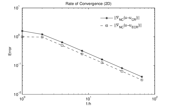
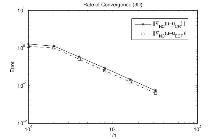
We compute two examples which compare the errors of the ECR and CR elements. The first example takes $\Omega=(0,1)^{2}$ and the exact solution $u(x,y)=\sin(\pi x)\sin(\pi y)$ ; the second takes $\Omega=(0,1)^{3}$ and the exact solution $u(x,y,z)=\sin(\pi x)\sin(\pi y)\sin(\pi z)$ . Both comparisons are illustrated in Figure 1, which indicates that $\|\nabla_{\rm NC}(u-u_{\rm ECR})\|$ is smaller than $\|\nabla_{\rm NC}(u-u_{\rm CR})\|$ .

Refer to caption — (a) $u(x,y)=\sin(\pi x)\sin(\pi y)$

5.2. Eigenvalue problem

We consider the eigenvalue problem (4.1). Since $V_{\rm CR}\subset V_{\rm ECR}$ , the eigenvalues produced by the ECR element are smaller than those by the CR element. When the meshsize is small enough, the ECR element has been proved to produce lower bounds for eigenvalues, see [21]. When eigenfunctions are singular, the CR element provides lower bounds for eigenvalues, see [2]; under some mesh conditions, it also produces lower bounds for eigenvalues when eigenfunctions are smooth, see [22].

On the coarse triangulation of the square domain $\Omega=(0,1)^{2}$ from Figure 2, the CR element produces a upper bound $\lambda_{\rm CR}=24$ for the first eigenvalue $\lambda=2\pi^{2}\approx 19.7392$ of the Laplace operator, while the ECR element gives a lower bound $\lambda_{\rm ECR}=17.1429$ .

Appendix A Basis Functions and Convergence Analysis of the ECR Element

For any $K\in\mathcal{T}$ , we give the basis functions of the shape function space ${\rm ECR}(K)$ . Suppose the coordinate of the centroid ${\rm mid}(K)$ is $(M_{1},M_{2}\cdots,M_{n})$ . The vertices of $K$ are denoted by $a_{i},1\leq i\leq n+1$ and the barycentric coordinates by $\lambda_{1},\lambda_{2},\cdots,\lambda_{n+1}$ . Let $H=\sum_{i<j}|a_{i}-a_{j}|^{2}$ , then the basis functions are as follows

\begin{split}&\phi_{K}=\frac{n+2}{2}-\frac{n(n+1)^{2}(n+2)}{2H}\sum^{n}_{i=1}(x_{i}-M_{i})^{2},\\ &\phi_{j}=1-n\lambda_{j}-\frac{1}{n+1}\phi_{K},\quad 1\leq j\leq n+1.\end{split}

For any $v\in V_{\rm ECR}$ , by the definition of $V_{\rm ECR}$ in (2.4), $\int_{E}[v]dE=0\text{ for all }E\in\mathcal{E}(\Omega)$ and $\int_{E}vdE=0\text{ for all }E\in\mathcal{E}(\partial\Omega)$ . From the theory of [23], there holds that

\|\nabla_{\rm NC}(u-u_{\rm ECR})\|\lesssim\|\nabla u-\Pi_{0}\nabla u\|+osc(f),

where

osc(f)=\left(\sum_{K\in\mathcal{T}}h_{K}^{2}\big[\inf_{\bar{f}\in P_{r}(K)}\|f-\bar{f}\|^{2}_{0,K}\big]\right)^{1/2}

$r\geq 0$ is arbitrary. The convergence of the ECR element follows immediately.

References

[1] T. Arbogast. Z. X. Chen. On the implementation of mixed methods as nonconforming methods for second order elliptic problems. Math. Comp., 64 (1995), pp. 943–972.
[2] M. G. Armentano and R. G. Duran. Asymptotic lower bounds for eigenvalues by nonconforming finite element methods. ETNA, 17 (2004), pp. 93–101.
[3] D. N. Arnold and F. Brezzi. Mixed and nonconforming finite element methods implementation, postprocessing and error estimates. RAIRO Modél. Math. Anal. Numér., 19 (1985), pp. 7–32.
[4] D. N. Arnold and R. S. Falk. A new mixed formulation for elasticity. Numer. Math., 53 (1988), pp. 13–30.
[5] I. Bab $\check{\rm u}$ ska, J. Osborn. Eigenvalue Problems. In: Handbook of Numerical Analysis, Vol. II, (P. G. Ciarlet and J. L. Lions, eds.), North Holland, 1991, pp. 641–787.
[6] D. Braess. An a posteriori error estimate and a comparison theorem for the nonconforming P1 element. Calcolo, 46 (2009), pp. 149–155.
[7] S. C. Brenner and L. R. Scott. The mathematical theory of finite element methods. Springer–Verlag, 1996.
[8] S. C. Brenner. A multigrid algorithm for the first order Raviart–Thomas mixed triangular finite element method. SIAM J. Numer. Anal., 29 (1992), pp. 647–678.
[9] Z. Cai, B. Lee, and P. Wang. Least–quares methods for incompressible Newtonian fluid flow: Linear stationary problems. SIAM J. Numer. Anal., 42 (2004), pp. 843–859.
[10] Z. Cai and Y. Wang. A multigrid method for the pseudostress formulation of Stokes problems. SIAM J. Sci. Comput., 29 (2007), pp. 2078–2095.
[11] C. Carstensen, D. Gallistl and M. Schedensack. Quasi–optimal adaptive pseudostress approximation of the Stokes equations. SIAM J. Numer. Anal., 51 (2013), pp 1715–1734.
[12] C. Carstensen and R. H. W. Hoppe. Convergence analysis of an adaptive nonconforming finite element method. Numer. Math., 103 (2006), pp. 251–266.
[13] C. Carstensen and R. H. W. Hoppe. Error reduction and convergence for an adaptive mixed finite element method. Math. Comp., 75 (2006), pp. 1033–1042.
[14] C. Carstensen, D. Kim, and E. J. Park. A priori and a posteriori pseudostress-velocity mixed finite element error analysis for the Stokes problem. SIAM J. Numer. Anal., 49 (2011), pp. 2501–2523.
[15] C. Carstensen, D. Peterseim, and M. Schedensack. Comparison results of finite element methods for the Poisson model problem. SIAM J. Numer. Anal., 50 (2012), pp. 2803–2823.
[16] M. Crouzeix and P. A. Raviart. Conforming and Nonconforming finite element methods for solving the stationary Stokes equations. RAIRO Anal. Numér., 7 R-3 (1973), pp. 33–76.
[17] R. G. Dur $\acute{a}$ n , L. Gastaldi and C. Padra. A posteriori error estimators for mixed approximations of eigenvalue problems. Math. Mod. Meth. Appl. Sci., 9 (1999), 1165–1178.
[18] T. Gudi. A new error analysis for discontinuous finite element methods for linear elliptic problems. Math. Comp., 79 (2010), pp. 2169–2189.
[19] K. Hellan. Analysis of elastic plates in flexure by a simplified finite element method. Acta Polytech. Scand. Civil Engrg. Ser., 46 (1967), pp. 1–28.
[20] L. Herrmann. Finite element bending analysis for plates. J. Eng. Mech. Div. ASCE, 93 (1967), pp. 13–26.
[21] J. Hu, Y. Q. Huang and Q. Lin. Lower Bounds for Eigenvalues of Elliptic Operators: By Nonconforming Finite Element Methods. J. Sci. Comput. DOI 10.1007/s10915-014-9821-5.
[22] J. Hu, Y. Q. Huang and Q. Shen. The Lower/Upper Bound Property of Approximate Eigenvalues by Nonconforming Finite Element Methods for Elliptic Operators. J. Sci. Comput., (58) 2014, pp. 574–591.
[23] J. Hu, R. Ma and Z. C. Shi. A new a priori error estimate of nonconforming finite element methods. Sci. China Math., (57) 2014, pp. 887–902.
[24] J. Hu and J. C. Xu. Convergence of Adaptive Conforming and Nonconforming Finite Element Methods for the Perturbed Stokes Equation, Research Report (2007), School of Mathematical Sciences and Institute of Mathematics, Peking University. (Also available online from December 2007: http://www.math.pku.edu.cn:8000/var/preprint/7297.pdf.)
[25] C. Johnson. On the convergence of a mixed finite element method for plate bending problems. Numer. Math., 21 (1973), pp. 43–62.
[26] L. D. Marini. An inexpensive method for the evaluation of the solution of the lowest order Raviart-Thomas mixed method. SIAM J. Numer. Anal., 22 (1985), pp. 493–496.
[27] S. Mao and Z. C. Shi. On the error bounds of nonconforming finite elements. Sci. China Math., 53 (2010), pp. 2917–2926.
[28] B. Mercier, J. Osborn, J. Rappaz, P. A. Raviart. Eigenvalue approximation by mixed and hybrid methods. Math. Comp., 36 (1981), pp. 427–453.
[29] L. S. D. Morley. The triangular equilibrium element in the solutions of plate bending problem. Aero. Quart., 19 (1968), pp. 149–169.
[30] P. A. Raviart and J. M. Thomas. A mixed finite element method for 2nd order elliptic problems. In: Mathematical Aspects of Finite Element Methods (I. Galligani and E. Magenes, eds.), Lecture Notes in Math. 606, Springer, Berlin, 1977, pp. 292–315.