Nonparametric Density Estimation Using Partially Rank-Ordered Set Samples With Application in Estimating the Distribution of Wheat Yield
Abstract
We study nonparametric estimation of an unknown density function based on the ranked-based observations obtained from a partially rank-ordered set (PROS) sampling design. PROS sampling design has many applications in environmental, ecological and medical studies where the exact measurement of the variable of interest is costly but a small number of sampling units can be ordered with respect to the variable of interest by any means other than actual measurements and this can be done at low cost. PROS observations involve independent order statistics which are not identically distributed and most of the commonly used nonparametric techniques are not directly applicable to them. We first develop kernel density estimates of based on an imperfect PROS sampling procedure and study its theoretical properties. Then, we consider the problem when the underlying distribution is assumed to be symmetric and introduce some plug-in kernel density estimators of . We use an EM type algorithm to estimate misplacement probabilities associated with an imperfect PROS design. Finally, we expand on various numerical illustrations of our results via several simulation studies and a case study to estimate the distribution of wheat yield using the total acreage of land which is planted in wheat as an easily obtained auxiliary information. Our results show that the PROS density estimate performs better than its SRS and RSS counterparts.
Keywords: Imperfect subsetting; Kernel function; Mean integrated square error; Nonparametric procedure; Optimal bandwidth; Ranked set sampling.
1 Introduction
Nonparametric density estimation techniques are widely used to construct an estimate of a density function and to provide valuable information about several features of the underlying population (e.g., skewness, multimodality, etc.) without imposing any parametric assumptions. These methods are very popular in practice and their advantages over histograms or parametric techniques are greatly appreciated. For example, they are widely used for both descriptive and analytic purposes in economics to examine the distribution of income, wages and poverty (e.g., Minoiu and Reddy, 2012); in environmental and ecological studies (e.g., Fieberg , 2007); or in medical research (e.g., Miladinovic et al. ), among others.
Most of these density estimation techniques are based on simple random sampling (SRS) design which involve independent and identically distributed (i.i.d.) samples from the underlying population. There are only a few results available when the sampling design is different (e.g., Buskrik, 1998; Chen, 1999; Gulati, 2004; Lam et al., 2002; Barabesi and Fattorini, 2002; Breunig, 2001, 2008; Opsomer and Miller, 2005). The properties of nonparametric kernel density estimation based on i.i.d. samples are well known and extensively studied in the literature (e.g., Wand and Jones, 1995; Silverman, 1986). In many applications, however, the data sets are often generated using more complex sampling designs and they do not meet the i.i.d. assumption. Examples include the rank-based sampling techniques which are typically used when a small number of sampling units can be ordered fairly accurately with respect to a variable of interest without actual measurements on them and this can also be done at low cost. This is a useful property since, quite often, exact measurements of these units can be very tedious and/or expensive. For example, for environmental risks such as radiation (soil contamination and disease clusters) or pollution (water contamination and root disease of crops), exact measurements require substantial scientific processing of materials and a high cost as a result, while the variable of interest from a small number of experimental (sampling) units may easily be ranked. These rank-based sampling designs provide a collection of techniques to obtain more representative samples from the underlying population with the help of the available auxiliary information. The samples obtained from such rank-based sampling designs often involve independent observations based on order statistics which are not identically distributed. So, it is important to develop kernel density estimators of the underlying population using such data sets and study their optimal properties.
In this paper, we study the problem of kernel density estimation based on a partially rank-ordered set (PROS) sampling design. Ozturk (2011) introduced PROS sampling procedure as a generalization of the ranked set sampling (RSS) design. To obtain a ranked set sample of size one can proceed as follows. A set of units is drawn from the underlying population. The units are ranked via some mechanism rather than the actual measurements of the variable of interest. Then, only the unit ranked as the smallest is selected for full measurement. Another set of units is drawn and ranked and only the unit ranked as the second smallest is selected for full measurement. This process is repeated times until the unit ranked the maximum is selected for the final measurement. See Chen et al. (2003), Wolfe (2004, 2012) and references therein for more details.
In RSS, rankers are forced to assign unique ranks to each observation even if they are not sure about the ranks. PROS design is aimed at reducing the impact of ranking error and the burden on rankers by not requiring them to provide a full ranking of all units in a set. Under PROS sampling technique, rankers have more flexibility by being able to divide the sampling units into subsets of pre-specified sizes based on their partial ranks. Ozturk (2011) obtained unbiased estimators for the population mean and variance using PROS samples. He also showed that PROS sampling has some advantages over RSS. Hatefi and Jafari Jozani (2013a, b) showed that the Fisher information of PROS samples is larger than the Fisher information of RSS samples of the same size. Since 2011, PROS sampling design has been the subject of many studies. Among others, see Gao and Ozturk (2012) for a two-sample distribution-free inference; Ozturk (2012) for quantile estimation; Frey (2012) for nonparametric estimation of the population mean; Arslan and Ozturk (2013) for parametric inference in a location-scale family of distributions, and Hatefi et al. (2013) for finite mixture model analysis based on PROS samples with a fishery application.
The outline of this paper is as follows. In Section 2 we introduce some preliminary results and present a general theory that can be used to obtain nonparametric estimates of some functionals of the underlying distribution based on imperfect PROS samples. In Section 3, we present a nonparametric kernel density estimate of the underlying distribution based on an imperfect PROS sampling scheme and study its properties. We also consider the problem of density estimation when the distribution of population is symmetric. In Section 4, we consider the problem of estimating the misplacement probabilities. To this end, we propose a modified EM-algorithm to estimate the probabilities of subsetting errors. This algorithm is fairly simple to implement and simulation results show that its performance is satisfactory. In Section 5, we compare our PROS density estimate with its RSS and SRS counterparts using simulation studies. Finally, in Section 6, we illustrate our proposed method by a real example.
2 Necessary backgrounds and preliminary results
In this section, we first give a formal introduction to PROS sampling design and then present some notations and preliminary results. Also, a general theory is obtained to provide nonparametric estimates of some functionals of the underlying distribution based on PROS samples.
2.1 PROS sampling design
To obtain a PROS sample of size , we choose a set size and a design parameter that partitions the set into mutually exclusive subsets, where and . First units are randomly selected from the underlying population and they are assigned into subsets , without actual measurement of the variable of interest and only based on visual inspection or judgment, etc. These subsets are partially judgment ordered, i.e. all units in subset judged to have smaller ranks than all units in , where . Then a unit is selected at random for measurement from the subset and it is denoted by . Selecting another units assigning them into subsets, a unit is randomly drawn from subset and then it is quantified and denoted by . This process is repeated until we randomly draw a unit form resulting in . This constitutes one cycle of PROS sampling technique. The cycle is then repeated times to generate a PROS sample of size , i.e. . Table 1 shows the construction of a PROS sample with and the design parameter . Each set includes four units assigned into two partially ordered subsets such that units in have smaller ranks than units in . In this subsetting process we do not assign any ranks to units within each subset so that they are equally likely to take any place in the subset. One unit, in each set from the bold faced subset, is randomly drawn and is quantified. The fully measured units are denoted by , ; .
| cycle | set | Subsets | Observation |
|---|---|---|---|
| 1 | |||
| 2 | |||
Note that if all units in have actually smaller ranks than all units in , then there is no subsetting error and the PROS sample is perfect. Otherwise, we have subsetting error and this PROS sample is called imperfect. To model an imperfect PROS sampling design, following Arslan and Ozturk (2013) and Hatefi and Jafari Jozani (2013a, b), let be a double stochastic misplacement probability matrix,
where is the misplacement probability of a unit from subset into subset with . Throughout the paper, we use to denote an imperfect PROS sampling design with subsetting error probability matrix , the number of subsets , the number of cycles , the set size , and the design parameter where , in which is the number of unranked observations in each subset. We note that SRS and imperfect RSS (with ranking error probability matrix ) can be expressed as special cases of the design when and , respectively. For a perfect PROS design, since for and for , we use , where is the identity matrix.
2.2 Some notations and preliminary results
In what follows, the probability density function (pdf) and cumulative distribution function (cdf) of the variable of interest are denoted by and , respectively. The pdf and cdf of , for , are denoted by and , respectively, and the pdf of the -th order statistic from a SRS of size is denoted by . We also use to denote and work with a second-order kernel density function that is symmetric and satisfies the following conditions
The SRS, RSS and PROS density estimates of are denoted by , and , respectively. Now, we present a useful lemma to show the connection between and .
Lemma 1.
Let denote a sample of size from a population with pdf and cdf , respectively. Then
| (4) |
where , and consequently
Remark 1.
For a design, we have
Therefore, a perfect PROS sample is a special case of an imperfect PROS sample and hence the results for a perfect PROS sampling can be obtained as a special case.
Let be a function of with . We study the method of moments estimate of by using an imperfect PROS sampling procedure, assuming that the required moments of exist. Note that different choices of lead to different types of estimators. For example, for , corresponds to the estimation of population moments; where is a kernel function and is a given constant, corresponds to the kernel estimate of pdf and , where is the indicator function of , corresponds to the estimate of cdf at point .
The method of moments estimate of based on an imperfect PROS sample of size is given by
| (5) |
The properties of is discussed in the following theorem.
Theorem 1.
Let be a sample of size from a population with pdf , and let the method of moments estimator of be defined as in (5). Then
- (i)
is an unbiased estimator of , i.e. .
- (ii)
where is the method of moments estimator of based on a SRS sample of comparable size.
- (iii)
is asymptotically distributed as a normal distribution with mean and variance as .
- (iv)
is a strong consistent estimator of as .
Proof.
The proof is essentially the same as the one given by Ozturk (2011) for which we present here for the sake of completeness. Part is an immediate consequence of Lemma 1. For part , using Ozturk (2011), we have
where . Note that the equality holds if and only if for all ; i.e. the subsetting process is purely random. For part , note that , where . However, for a fixed , converges asymptotically to a normal distribution with mean and variance as by the Central Limit Theorem. Therefore, the result holds for . Finally, part follows from the Strong Law of Large Numbers. ∎
3 Kernel density estimate based on PROS samples
In this section, we present a kernel density estimator of based on an imperfect PROS sample of size and study some theoretical properties of our proposed estimator. Also, we consider the problem of density estimation when is assumed to be symmetric.
3.1 Main results
To obtain a PROS kernel density estimator of we first note that from Lemma 1 we have . For a fixed , the sub-sample can be considered as a simple random sample of size from . Hence, can be estimated by the usual kernel method as follows
| (6) |
where is the bandwidth to be determined. We propose a kernel estimate of as
| (7) |
Now, we establish some theoretical properties of . To this end, let be a kernel density estimator of based on a SRS of size and note that (e.g., Silverman, 1986)
and
| (8) |
Theorem 2.
Suppose that is a kernel density estimator of based on a sample of size and let denote its corresponding SRS kernel estimator based on a SRS sample of the same size. Then,
- (i)
,
- (ii)
, where
in which is an observation obtained from a design.
- (iii)
at a fixed point is distributed asymptotically as a normal distribution with mean and variance for large .
Proof.
The results hold immediately from Theorem 1 by letting . ∎
Theorem 2 shows that has the same expectation as and a smaller variance than . This implies that has a smaller mean integrated square error (MISE) than , that is
In addition, by using part of Theorem 2, one can construct an asymptotic pointwise confidence interval for as follows
where is the -th quantile of the standard normal distribution and
where is a consistent estimators of given by (6).
Note that our estimate depends on a bandwidth which should be determined in practice. We present an asymptotic optimal bandwidth by minimizing the asymptotic expansion of MISE. In this regard, we first present a lemma which is useful for obtaining the asymptotic expansion of MISE.
Lemma 2.
Assuming that the underlying density is sufficiently smooth with desired derivatives and is a second-order kernel function, for a fixed , as , we have
Proof.
Using (4) and by changing the variable , we have
Replacing by its Taylor expansion and using the properties of the kernel function , one can easily get
Consequently,
and it is similarly verified that
which completes the proof. ∎
Theorem 3.
Suppose that the same bandwidth is used in both and . Then, for large ,
where .
Proof.
Theorem 3 shows that the optimal bandwidth which minimizes MISE, asymptotically minimizes MISE up to order . That is, one can use the following optimal bandwidth which is obtained by minimizing asymptotical expansion of MISE
(see Chen (1999)). The optimal bandwidth depends on which is unknown and, in practice, a nonparametric version of it can be used (see Silverman (1986)). Theorem 3 also shows that the PROS estimate reduces the MISE of SRS estimate at order , and the amount of this reduction asymptotically is (note that is non-negative). Unfortunately, the value of depends on ; however, as we show below, one can characterize asymptotic rate of this reduction in a perfect PROS sampling procedure as an upper bound for .
Lemma 3.
Under a sampling design,
where and are i.i.d. binomial random variables with parameters and , i.e. .
Proof.
Using Remark 1, one can easily verify that
where . Let for . Since is also distributed as a distribution and it is independent of , then
since s constitute a disjoint partition of the set and this completes the proof. ∎
By Lemma 3, we can derive an asymptotic result which provides more insight into the rate of reduction in MISE in a perfect PROS sampling procedure.
Theorem 4.
Under a sampling design, we have
where .
Proof.
Note that by the Edgeworth expansion of in Lemma 3, we get
Consequently, we can write
and this completes the proof. ∎
Theorem 4 shows that a perfect PROS density estimate reduces the MISE of at order and this reduction is increased by linearly whenever is non-negative (a sufficient condition is ). When , the result is reduced to the result for perfect RSS density estimate given by Chen (1999). In Section 5, we compare with and in a more general case where the sampling procedure can be either perfect or imperfect.
3.2 Density estimation under symmetry assumption
In this section, we consider the problem of kernel density estimation based on an imperfect PROS sample of size under the assumption that is symmetric. To this end, suppose that is symmetric about , that is for all . One can easily verify that provided for all . Therefore, based on the sub-sample , it is reasonable to estimate by
where is given in (6). Consequently, the estimate of under the symmetry assumption can be defined by
Now, we consider the mean and the variance of in the following theorem.
Theorem 5.
Suppose that is symmetric about and for all . Then, based on an imperfect sample of size , we have
- (i)
,
- (ii)
Proof.
Part is easily proved by the fact that under the symmetry assumption and Theorem 2. For part , note that for all , we have
and consequently
The result holds by using the Cauchy-Schwartz inequality. ∎
Theorem 5 shows that has the same bias as ; however, it has smaller variance. Therefore, under the symmetry assumption has smaller MISE and it dominates . Note also that if the symmetry point is unknown, it can be estimated by the PROS sample to obtain a plug-in estimator as . Based on a PROS sample of size , several non-parametric estimators of can be defined as follows
| (10) |
Among these estimators is the PROS sample mean which is not robust against outliers, while , , and are robust estimators of . Note that is a Hodges-Lehmann type estimator of the location parameter. In Section 5, we consider the effect of these estimators on the MISE of .
4 Estimating the misplacement probabilities
So far we assumed that the misplacement probability matrix defined in (2.1) is given. In practice, the misplacement probabilities are unknown and they should always be estimated. This is a very important problem as the performance of our kernel density estimator depends on the estimated values of . In this section, we use a modification of the EM algorithm of Arsalan and Ozturk (2013) to estimate ’s. We present the result for a symmetric misplacement probability matrix with . However, results for more general can be obtained by slight modifications of our results. Let
in which
and denotes the pdf of a beta distribution with parameters and . Following Arslan and Ozturk (2013) we estimate the misplacement probability matrix through an iterative method. To this end, we start with an initial estimate of say which can be chosen to be a matrix associated with random subsetting with . Then, we use the following iterative method:
- (i)
For a given at step of the iterative process, calculate
- (ii)
Calculate
- (iii)
Maximize under the restrictions that the misplacement probabilities are symmetric and doubly stochastic and obtain the new and call it . This can be done via a Lagrange multipliers method to enforce the constraints as follows
where . The details of this process are given in Ozturk (2010) as well as Arslan and Ozturk (2013).
- (iv)
Repeat Steps (i)-(iii) till the sum of absolute error (SAE) of and is less than a predetermined value, say , that is
In practice, to calculate , one can replace by an estimate of such as the empirical distribution function, i.e.
To investigate the accuracy of our method, we perform a small simulation study when , and . Following Arslan and Ozturk (2013), we consider three misplacement probability matrices , , and , where
We generate PROS samples when the underlying population distributions are the standard Normal and Exponential distributions. For each distribution, the misplacement probabilities are estimated by using our proposed iterative method with the help of the package “Rsolnp” (Ghalanos and Theussl (2012) and Ye (1987)) in R with . This process is repeated 100 times and the average of these estimates are used as the estimates of the misplacement probabilities. The values of the estimates and their corresponding standard deviations (given in parentheses) are shown in Table 2. Note that following the properties of we present the results for , , , , and . We observe that the estimates are close to the true values and they have satisfactory biases given the fact that our proposed method is a fully nonparametric procedure and the sample size is very small. We observe that our proposed procedure slightly underestimates , especially for . This is because the perfect ranking model is at the boundary of the parameter space and as noted by Arslan and Ozturk (2013) the estimates are truncated whenever they exceed 1 due to the constraints on misplacement probabilities. However, the biases and standard deviations get smaller as the cycle size increases.
| Distributions | |||||||
|---|---|---|---|---|---|---|---|
| 4 | 0.9640(0.099) | 0.0355(0.097) | 0.0006(0.005) | 0.9179(0.155) | 0.0466(0.109) | ||
| 10 | 0.9775(0.051) | 0.0204(0.051) | 0.0021(0.012) | 0.9565(0.070) | 0.0232(0.054) | ||
| 4 | 0.8934(0.156) | 0.0717(0.140) | 0.0348(0.087) | 0.8247(0.198) | 0.1036(0.143) | ||
| Normal | 10 | 0.8961(0.106) | 0.0759(0.096) | 0.0280(0.044) | 0.8356(0.153) | 0.0886(0.102) | |
| 4 | 0.7578(0.207) | 0.1535(0.188) | 0.0888(0.116) | 0.6583(0.274) | 0.1882(0.217) | ||
| 10 | 0.7365(0.140) | 0.1605(0.137) | 0.1030(0.082) | 0.6902(0.174) | 0.1493(0.125) | ||
| 4 | 0.9384(0.134) | 0.0612(0.134) | 0.0004(0.004) | 0.8751(0.185) | 0.0637(0.139) | ||
| 10 | 0.9730(0.052) | 0.0265(0.052) | 0.0005(0.005) | 0.9501(0.068) | 0.0234(0.048) | ||
| 4 | 0.8918(0.167) | 0.0833(0.164) | 0.0249(0.059) | 0.7880(0.225) | 0.1287(0.158) | ||
| Exponential | 10 | 0.8802(0.107) | 0.0891(0.104) | 0.0307(0.042) | 0.8014(0.161) | 0.1095(0.112) | |
| 4 | 0.7486(0.232) | 0.1475(0.187) | 0.1039(0.136) | 0.6535(0.254) | 0.1990(0.204) | ||
| 10 | 0.7515(0.132) | 0.1513(0.125) | 0.0972(0.090) | 0.6893(0.173) | 0.1595(0.128) |
5 Simulation Study
In this section, we compare the performance of with its SRS and RSS counterparts. We first discuss the asymptotic reduction rate in the variance (RRV) of and by using a PROS density estimate . We then compare the MISE with MISE and MISE. Finally, we consider the effect of estimating the symmetry point on the MISE of when we assume that the underlying distribution is symmetric.
5.1 Comparing the reduction in variances
Using (9), the RRV of over that measures at what rate reduces the asymptotic variance of can be defined as
where . It is clear that is a nonparametric measure which does not depend on the underlying distribution function. Note that if RRV at certain percentiles , then and have equal variances at these percentiles asymptotically. However, if RRV, then reduces the variance of at order and this reduction increases linearly at rate . The values of RRV can be easily calculated when , and the misplacement probabilities are given. For and and misplacement probabilities and for , the values of RRV are presented in Figure 1 when .
We observe that for all values of the amount of RRV increases symmetrically as gets away from 0.5 to 0 and 1. This shows that the best performance of the PROS density estimate over its SRS counterpart happens at the tail of the distribution. When , the PROS and SRS estimates have equal precision at ; otherwise, the PROS estimate reduces the variance of SRS estimate. When , the value of RRV decreases when increases. This suggests using a small sample size when the misplacement probabilities (ranking errors) are large. We also note that RRV increases as both and increase. The best performance of PROS design over SRS design happens when the subsetting is either perfect or it is moderately good, that is when or , respectively. Similar results are observed when which we do not present here.
To obtain the RRV of over we first note that (see Chen (1999))
Now, using (9), the RRV of when is defined as
where
in which and for are the ranking error probabilities in an imperfect RSS procedure.

(a)


(c)

(d)
For , and the ranking error probabilities equal to the misplacement error probabilities in its corresponding imperfect PROS design, the values of RRV are presented in Figure 2. It is seen that the values of RRV are symmetric about . When , the RRV decreases as increases, and by increasing RRV of increases as increases. The RRV of RSS is zero when and 1 (when , the value of RRV is also zero at ). This means that the PROS and RSS estimates have the same precision at these percentiles. The maximum value of RRV is more than 35 percent when the sampling procedure is perfect and . Similar results are obtained when which are not presented here.
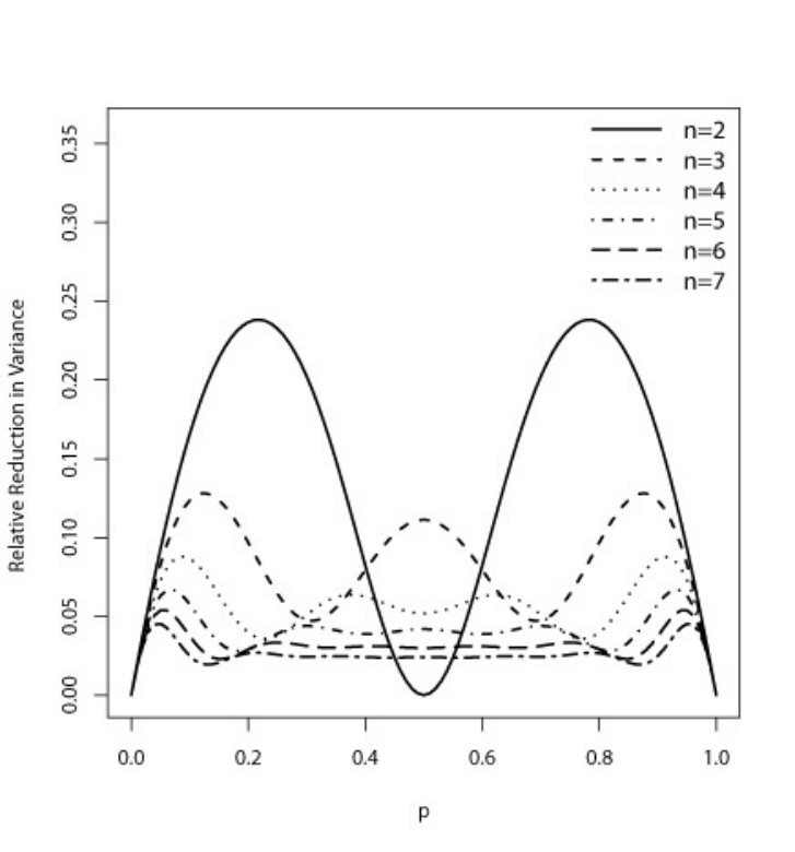
(a)
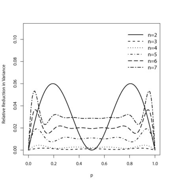
(b)
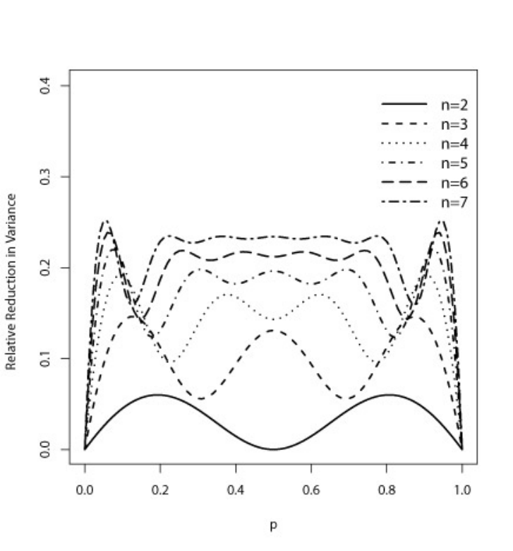
(c)
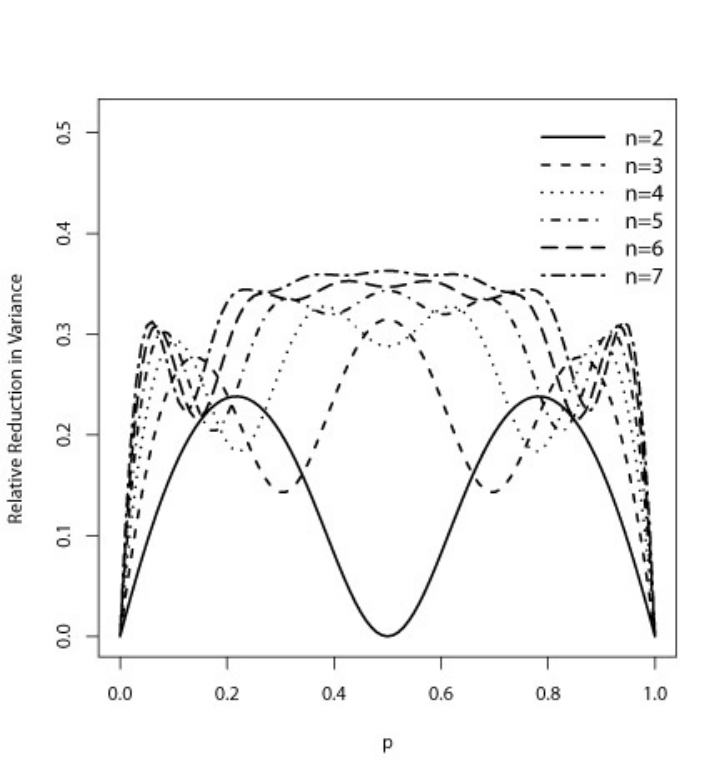
(d)
5.2 Comparing MISE’s of , and
In order to compare MISE with MISE and MISE, following Chen (1999), we consider (a) the standard Normal distribution, (b) the Gamma distribution with shape parameter 3 and scale parameter 1, and (c) the standard Gumbel distribution. We use the Epanechnikov kernel in all estimates and the bandwidth is determined by
where ; see Silverman (1986). For given , , and different misplacement probabilities, we use the following procedure to estimate the values of MISE, MISE, and MISE. For each estimator, the integrated square error (ISE) is calculated based on the corresponding SRS, imperfect RSS and imperfect PROS samples. Then, the ISE of 5,000 PROS, RSS, and SRS estimates is obtained. For each procedure, the average of these 5,000 ISEs is used as an estimate of the corresponding MISEs. The ratios
are obtained as the efficiency of with respect to and , respectively. Table 3 shows the values of RP and SP for these distributions with different values of , , , and .
| 0 | 0.3 | 0.5 | 0.7 | 1 | |||
| Distributions | (RP , SP) | (RP , SP) | (RP , SP) | (RP , SP) | (RP , SP) | ||
| 6 | 4 | (1.012,1.030) | (1.000,0.993) | (1.022,1.084) | (1.100,1.281) | (1.399,2.151) | |
| 6 | 8 | (1.026,1.058) | (1.015,1.015) | (1.041,1.093) | (1.099,1.268) | (1.309,1.960) | |
| Normal | 8 | 3 | (0.997,0.991) | (1.008,1.008) | (1.044,1.128) | (1.113,1.337) | (1.408,2.453) |
| 8 | 6 | (0.998,1.014) | (1.006,1.018) | (1.042,1.119) | (1.106,1.310) | (1.398,2.265) | |
| 6 | 4 | (1.021,1.022) | (1.004,1.009) | (1.010,1.069) | (1.060,1.190) | (1.233,1.650) | |
| 6 | 8 | (1.005,1.007) | (1.013,1.014) | (1.033,1.061) | (1.059,1.159) | (1.160,1.486) | |
| Gamma | 8 | 3 | (1.018,1.054) | (0.992,1.010) | (1.025,1.113) | (1.077,1.278) | (1.224,1.811) |
| 8 | 6 | (1.009,0.998) | (1.002,0.995) | (1.022,1.063) | (1.071,1.195) | (1.173,1.546) | |
| 6 | 4 | (0.985,1.040) | (0.984,1.023) | (1.013,1.095) | (1.102,1.284) | (1.283,1.866) | |
| 6 | 8 | (1.007,0.999) | (1.016,0.990) | (1.058,1.064) | (1.074,1.172) | (1.239,1.619) | |
| Gumbel | 8 | 3 | (1.022,1.002) | (0.992,1.010) | (1.031,1.099) | (1.070,1.265) | (1.269,1.936) |
| 8 | 6 | (0.996,0.984) | (1.009,1.007) | (1.037,1.075) | (1.092,1.208) | (1.237,1.738) | |
Form Table 3, it is seen that as the misplacement probabilities decrease the efficiency of PROS with respect to RSS and SRS increases and, as we expect, the efficiency with respect to SRS is more than RSS procedure. When the misplacement probabilities are large, , the three estimators have efficiency near one. The efficiency of PROS with respect to RSS and SRS increases slightly as increases (this increment is faster when , results in which are not presented here); however, the efficiency decreases as increases. The amount of efficiency for the Normal distribution is higher than the Gamma and Gumbel distributions. For example, when , , and the efficiencies of PROS with respect to SRS for the Normal, Gamma, and Gumbel distributions are , , and , respectively. We observe that the main parameter that controls the efficiency is the misplacement probability matrix or equivalently the ranking error. When the ranking errors are high, there is no substantial difference between , , and . However, as the ranking errors decrease, our simulation results show that the PROS density estimate performs better than RSS and SRS density estimates in terms of MISE.
5.3 Results under symmetry assumption
To investigate the effect of estimating the symmetry point on the MISE of , we consider four distributions (a) the standard Normal and (b) Logistic distributions as light tail distributions, (c) t-student with 2 degrees of freedom, and (d) the standard Laplace distributions as heavy tail distributions. For each distribution, a perfect PROS sample of size with subset size are generated and the four symmetry point estimators given in (4) were calculated. Then, MISE and MISE for , , were calculated and their ratios are obtained as the efficiency of ’s with respect to . The results for , , and are shown in Table 4. The last column shows the efficiency of with respect to when the symmetry point is known.
We observe that performs the best in all cases which suggests using the Hodges-Lehmann type estimator, , for estimating the symmetry point. For Normal distribution, the efficiencies of and with respect to are competitive. However, for distribution, which is a heavy tail distribution, it does not hold. On the other hand, the efficiencies of and with respect to are very close especially in heavy tail distributions. Generally, we recommend using when it is assumed that the underlying population distribution is symmetric. Comparing the efficiencies of and with respect to indicates how much the efficiency reduces when the symmetry point is estimated. This reduction is larger when in comparison with (the maximum value of reduction is about when and in Normal distribution and the minimum value is when and in Laplace distribution).
| Estimators | |||||||
|---|---|---|---|---|---|---|---|
| Distributions | |||||||
| 6 | 3 | 1.176 | 1.062 | 1.212 | 1.155 | 1.364 | |
| 6 | 4 | 1.185 | 1.057 | 1.225 | 1.165 | 1.353 | |
| Normal | 8 | 3 | 1.161 | 1.031 | 1.205 | 1.125 | 1.313 |
| 8 | 4 | 1.173 | 1.054 | 1.219 | 1.146 | 1.309 | |
| 6 | 3 | 1.103 | 1.098 | 1.198 | 1.172 | 1.339 | |
| 6 | 4 | 1.102 | 1.104 | 1.207 | 1.185 | 1.339 | |
| Logistic | 8 | 3 | 1.108 | 1.095 | 1.205 | 1.159 | 1.307 |
| 8 | 4 | 1.108 | 1.092 | 1.205 | 1.162 | 1.293 | |
| 6 | 3 | 0.675 | 1.150 | 1.191 | 1.201 | 1.299 | |
| 6 | 4 | 0.645 | 1.133 | 1.182 | 1.190 | 1.284 | |
| t(2) | 8 | 3 | 0.621 | 1.133 | 1.186 | 1.176 | 1.268 |
| 8 | 4 | 0.615 | 1.129 | 1.185 | 1.176 | 1.257 | |
| 6 | 3 | 0.998 | 1.130 | 1.151 | 1.158 | 1.234 | |
| 6 | 4 | 1.002 | 1.119 | 1.141 | 1.146 | 1.217 | |
| Laplace | 8 | 3 | 1.007 | 1.112 | 1.139 | 1.135 | 1.193 |
| 8 | 4 | 1.011 | 1.108 | 1.131 | 1.129 | 1.172 | |
6 Real Data Application
In this section, we illustrate our method with a real data set collected by the Iranian Ministry of Jihade-Agricultural (IMJA) in 2005. Jafari Jozani et al. (2012) used this data set in a different context to examine the accuracy of several ratio estimators of the population mean based on RSS design. The data set contains the information of the wheat yield and the total acreage of land which is planted in wheat for 304 cities in 31 provinces of Iran in 2005. Wheat yield estimation is important for advanced planning and implementation of policies related to food distribution, import-export decision, etc. We provide kernel density estimates of the distribution of = wheat yield (in ton) as the variable of interest by using = total acreage of the planted land in wheat (in acre) as the auxiliary variable which can be used for the ranking purpose. The correlation coefficient between and is 0.786. For ease of computations, we divided the values of by 100,000,000.
In order to estimate the density function of wheat yield, we regarded this data set as a population and extracted PROS, RSS and SRS with replacement samples of size from the population. For each design, the density estimates are obtained and the asymptotic variance estimates are calculated. Then, this process is repeated times and the average of density estimates at a fixed point are considered as the density estimates. In addition, for each design, the average of asymptotic variance estimates are also calculated for constructing asymptotic pointwise confidence bounds. We take , , and . The histogram of 304 records of is shown in Figure 3. The PROS density estimate and its 95 percent asymptotic pointwise confidence bounds are shown in third column of Figure 3. The SRS and RSS density estimates and their corresponding 95 percent pointwise confidence bounds are also shown in the 1st and 2nd columns of Figure 3. In all cases, we used Epanechnikov kernel and the bandwidth was determined as in Section 5.2. To obtain the probabilities of subsetting errors, we used the proposed algorithm in Section 4. We estimated the probabilities of subsetting errors for each 20 samples with SAE=0.001. The average of these estimates are given below
The standard deviations of the estimates vary between 0.05 and 0.19. Our estimates show that the probabilities of correct subsetting are much higher than the probabilities of incorrect subsetting and this is due to the fact that and are highly correlated. We observe that the density estimates look similar. However, the confidence bounds for PROS design are much narrower than the confidence bounds obtained by SRS and RSS designs.

Acknowledgments
Mohammad Jafari Jozani gratefully acknowledges the research support of the Natural Sciences and Engineering Research Council of Canada.
References
- (2) Arslan, G. and Ozturk, O. (2013). Parametric inference based on partially rank ordered set samples. Journal of the Indian Statistical Association, 51, 1–24.
- (4) Barabesi, L. and Fattorini, L. (2002). Kernel estimation of probability density functions by ranked set sampling. Communication in Statistics: Theory and Methods, 31, 597–610.
- (6) Breunig, R.V. (2001). Density estimation for clustered data. Econometric Reviews, 20, 353–367.
- (8) Breunig, R.V. (2008). Nonparametric density estimation for stratified samples. Statistics and Probability Letters, 78, 2194–2200.
- (10) Buskirk, T.D. (1998). Nonparametric density estimation using complex survey data. In ASA Proceedings of the Section on Survey Research Methods, 799–801. American Statistical Association.
- (12) Chen, Z., Bai, Z. and Sinha, B.K. (2003). Ranked Set Sampling: Theory and Applications. Springer-Verlag, New York.
- (14) Chen, Z. (1999). Density estimation using ranked set sampling data. Environmental and Ecological Statistics, 6, 135–146.
- (16) Fieberg, J. ( 2007). Kernel density estimators of home range: smoothing and the autocorrelation red herring. Ecology, 88, 1059–1066.
- (18) Frey, J. (2012). Nonparametric mean estimation using partially ordered sets. Environmental and Ecological Statistics, 6, 309–326.
- (20) Gao, J.L. and Ozturk, O. (2012). Two sample distribution-free inference based on partially rank-ordered set samples. Statistics and Probability Letters, 82, 876–884.
- (22) Ghalanos, A. and Theussl, S. (2012). Rsolnp: General Non-linear Optimization Using Augmented Lagrange Multiplier Method. R package version 1.14.
- (24) Gulati, S. (2004). Smooth non-parametric estimation of the distribution function from balanced ranked set samples. Environmetric, 15, 529–539.
- (26) Hatefi, A., Jafari Jozani, M. and Ozturk, M. (2014). Mixture model analysis of partially rank ordered set samples: Estimating the age-groups of fish from length-frequency data. submitted.
- (28) Hatefi, A. and Jafari Jozani, M. (2013a). Information content of partially rank ordered set samples. submitted.
- (30) Hatefi, A. and Jafari Jozani, M. (2013b). Fisher information in different types of perfect and imperfect ranked set samples from finite mixture models. Journal of Multivariate Analysis, 119, 16–31.
- (32) Jafari Jozani, M., Majidi, S. and Perron, F. (2012). Unbiased and almost unbiased ratio estimators of the population mean in ranked set sampling. Statistical Papers, 53, 719–737.
- (34) Lam, K.F., Yu, P.L.H., and Lee, C.F. (2002). Kernel method for the estimation of the distribution function and the mean with auxiliary information in ranked set sampling. Environmetrics, 13, 397–406.
- (36) Minoiu, C. and Reddy, S.G. (2012). Kernel density estimation on grouped data: the case of poverty assessment. The Journal of Economic Inequality. To appear.
- (38) Opsomer, J. D. and C. P. Miller (2005). Selecting the amount of smoothing in nonparametric regression estimation for complex surveys. Journal of Nonparametric Statistics, 17, 593–611.
- (40) Ozturk, O. (2012). Quantile inference based on partially rank ordered set samples. Journal of Statistical Planning and Inference, 142, 2116–2127.
- (42) Ozturk, O. (2011). Sampling from partially rank-ordered sets. Environmental Ecological Statistics, 18, 757–779.
- (44) Miladinovic, B., Kumar, A., and Djulbegovic, B. (2013). Kernel Density Estimation for Random-effects Meta-analysis. International Journal of Mathematical Sciences in Medicine, 1, 1–5.
- (46) Silverman, B.W. (1986). Density Estimation for Statistics and Data Analysis. Chapman and Hall, London, New York.
- (48) Wand, M.P., and Jones, M.C. (1995). Kernel smoothing. Chapman and Hall, London.
- (50) Wolfe, D.A. (2012). Rank set sampling: Its relevance and impact on statistical inference. ISRN Probability and Statistics, doi 10.5402/2012/568385.
- (52) Wolfe, D.A. (2004). Ranked set sampling: An approach to more efficient data collection. Statistical Science, 19, 636–643.
- (54) Ye, Y. (1987). Interior algorithms for linear, quadratic, and linearly constrained non-linear programming. Ph.D. Thesis, Department of EES, Stanford University.