Quasi-One Dimensional Models for Glassy Dynamics
Abstract
We describe numerical simulations and analyses of a quasi-one-dimensional (Q1D) model of glassy dynamics. In this model, hard rods undergo Brownian dynamics through a series of narrow channels connected by intersections. We do not allow the rods to turn at the intersections, and thus there is a single, continuous route through the system. This Q1D model displays caging behavior, collective particle rearrangements, and rapid growth of the structural relaxation time, which are also found in supercooled liquids and glasses. The mean-square displacement for this Q1D model displays several dynamical regimes: 1) short-time diffusion , 2) a plateau in the mean-square displacement caused by caging behavior, 3) single-file diffusion characterized by anomalous scaling at intermediate times, and 4) a crossover to long-time diffusion for times that grow with the complexity of the circuit. We develop a general procedure for determining the structural relaxation time , beyond which the system undergoes long-time diffusion, as a function of the packing fraction and system topology. This procedure involves several steps: 1) define a set of distinct microstates in configuration space of the system, 2) construct a directed network of microstates and transitions between them, 3) identify minimal, closed loops in the network that give rise to structural relaxation, 4) determine the frequencies of ‘bottleneck’ microstates that control the slow dynamics and time required to transition out of them, and 5) use the microstate frequencies and lifetimes to deduce . We find that obeys power-law scaling, , where both (signaling complete kinetic arrest) and depend on the system topology.
pacs
64.70.kj, 61.43.Fs, 82.70.DdI Introduction
Developing a fundamental understanding of glass transitions in amorphous materials is one of the remaining grand challenges in condensed matter physics [1, 2, 3]. Glass transitions occur in myriad systems including atomic, magnetic, polymer, and colloidal systems. Hallmarks of the glass transition include a stupendous increase in the structural and stress relaxation times [4] and a concomitant dramatic decrease in the mobility over an extremely narrow range of temperature or density, broad distributions of particle motions that are spatially and temporally heterogeneous, and aging behavior in which the system becomes progressively more viscous with time after it has been quenched to the glassy state [5].
Glass transitions in liquids show marked similarities to jamming transitions in athermal systems such as granular media, foams, and emulsions that do not thermally fluctuate [6]. Athermal systems typically jam, or develop a nonzero static shear modulus, at sufficiently large densities or confining pressures, and remain jammed for applied shear stresses below the yield stress. Similarities between jammed and glassy systems include highly cooperative and heterogeneous particle motion in response to perturbations [7, 8] and extremely slow relaxation [9] as a system approaches the glass or jamming transition.
Dense colloidal suspensions undergo a glass transition when they are compressed to packing fractions approaching random close packing (provided they are compressed rapidly or are sufficiently polydisperse) [10]. Random close-packed states are amorphous, mechanically stable sphere packings with for monodisperse spheres [11, 6]. In Fig. 1, we show the mean-square displacement (MSD) versus time over a range of from to from molecular dynamics (MD) simulations of polydisperse [12], elastic hard spheres with ballistic (not Brownian) short-time dynamics. This data was obtained from studies by M. Tokuyama and Y. Terada, and is similar to results in Refs. [13, 14, 15]. For relatively dilute systems, the MSD crosses over from ballistic () to diffusive () when it reaches , where is the average particle diameter. The formation of a plateau in the MSD (for ) signals the onset of caging behavior, where particles are trapped by neighboring particles that surround them. The height and length of the plateau characterize the cage size and the time over which caging persists. The appearance of the plateau and two-stage relaxation in the MSD leads to dramatic increases in the structural and stress relaxation times as shown in Fig. 2. In this figure, we demonstrate that the structural relaxation time (time beyond which the MSD scales as grows by nearly four orders of magnitude over a small range in packing fraction.
Because of the rapid rise in relaxation times and the fact that dense colloidal systems can only be equilibrated at packing fractions well below random close-packing, it is difficult to accurately measure the precise form of the divergence of the relaxation times [16]. In particular, there is current vigorous debate concerning the packing fraction at which complete dynamical arrest occurs—is it before random close packing or does dynamic arrest coincide with random close packing [17]? If it is the former, it is possible that these systems undergo an ideal glass transition to a static, but not mechanically stable state. Further open questions include determining the collective particle motions that are responsible for subdiffusive behavior and the onset of super-Arrhenius dynamics, which occur well below random close packing.

There have been a number of theoretical and computational studies aimed at understanding slow dynamics in dense colloidal suspensions and related glassy systems [18, 19, 20, 21]. These include the application of mode coupling theory to colloidal systems [22] and the development of coarse-grained facilitated [23] and kinetically constrained lattice models [24, 25]. Mode coupling theory has been successful in predicting the form of the two-step relaxation of the intermediate scattering function, but it predicts an ergodicity-breaking transition well-above the experimentally determined colloidal glass transition. Related theories are able to predict activated dynamics, but the location of the divergence in the structural and stress relaxation times is still an input parameter, not a prediction [26]. Models of dynamic facilitation, in which mobile regions increase the probability that nearby regions will also become mobile, are able to explain important aspects of dynamical heterogeneities and non-Arrhenius relaxation times. However, these models have been implemented using either coarse-grained or lattice descriptions, not particle-scale, continuum models.

Even though researchers have been able to visualize the motions of colloidal particles in 3D using confocal microscopy for more than a decade [27, 28], an understanding of the particle-scale origins of dynamical heterogeneities, cage formation and relaxation, and structural rearrangements that give rise to subdiffusive behavior is lacking. Several factors have contributed to the slow progress. First, it is well-known that it is difficult to predict dynamical quantities from static structural properties. Thus, even though one can visualize all colloidal particles in 3D, it is difficult to determine in advance which particles will move cooperatively. Further, it has proved difficult to identify and sample the rare transition states that allow the system to move from one region in configuration space to another.
We have developed a quasi-one-dimensional (Q1D) model, where hard rods diffuse through a series of connected loops and junctions (or intersections) [29] as shown in Fig. 3. There are a number of advantages for employing this model to explore slow dynamics in colloidal and other glassy systems. First, this model displays many features of glassy behavior including caging, heterogeneous and collective dynamics, and a divergence of the structural relaxation time . Second, the form of the divergence of with increasing packing fraction can be determined analytically. Third, simulations and experiments of the colloidal glass transition show evidence for quasi-one-dimensional behavior such as correlated string-like motion of the fastest moving particles [30, 31] and subdiffusive behavior with MSD that is characteristic of single-file diffusion in quasi-one-dimensional systems [32, 33]. For example, possible single-file subdiffusive behavior occurs in simulations of polydisperse, elastic hard-sphere systems for packing fractions and as shown in Fig. 1.

In our previous studies of quasi-one dimensional models, we focused on the ‘figure-8’ system with a single junction (or intersection) [29] and hard rods. We found that the structural relaxation time diverges as a power-law with increasing packing fraction,
| (1) |
where and is the packing fraction at which kinetic arrest occurs. At kinetic arrest, a plateau in the MSD persists for . Near , the most likely configurations are those with particles in both the top and bottom end lobes, and no particles in the junction. is controlled by rare ‘junction-crossing’ events, in which a particle from the bottom (top) lobe, crosses the junction, enters the top (bottom) lobe from one side of the junction, and another particle exits the top (bottom) lobe and enters the bottom (top) lobe from the other side of the junction. Thus, to undergo structural relaxation, the system transitions from a relaxed configuration with half of the particles in each lobe to a rare, squeezed configuration with an extra particle in one of the lobes, and back to a relaxed configuration that is similar to the initial one but with particle labels shifted forward or backward by one. The frequency of junction-crossing events is determined by the probability for a squeezed configuration to occur divided by the residence time that the system spends in the squeezed configuration ,
| (2) |
The structural relaxation time is the inverse of this frequency, and thus . If we assume ergodicity, can be calculated from configuration integrals, and for the figure-8 model, , where is the number of particles in the squeezed lobe. The residence time for the squeezed configuration in the figure-8 model tends to zero in the limit , and thus as in Eq. 1.
II Model Description
II.1 System geometry
We consider the collective dynamics of non-overlapping Brownian particles in a quasi-one-dimensional (Q1D) channel that forms a closed loop with multiple intersections, as illustrated in Fig. 3. The particles move through the intersections in mode I in the first half of the circuit and mode II in the second half. For systems with multiple intersections, modes and alternate between the northeast/southwest (NE/SW) and northwest/southeast (NW/SE) directions. The particles can move in both the forward and backward directions, but they cannot turn at the intersections. Thus, to switch the traffic mode at a given intersection, particles in one mode must vacate the junction to allow particles in the other mode to enter.

The topology of the system is characterized by the number of junctions . Each channel has two end lobes, and for a given there are symmetric middle lobes. The channel geometry is described by three length parameters: the channel width (which also determines the length of the intersection), and the length of the end and middle lobes and .
To reduce the number of independent parameters we focus on a model with
| (3) |
We also assume that the particle size is equal to the channel width,
| (4) |
With these assumptions, exactly particles fit into a middle lobe and particles fit into an end lobe when , where is an integer.
With the lengths of the middle and end lobes related by Eq. (3), the total length of the channel is
| (5) |
where the length of each intersection is counted both in the NE and NW directions. The packing fraction of the particles in the channel is given by
| (6) |
In our intersecting-channel model, particles moving through an intersection in one direction block the motion of particles in the perpendicular direction. Thus, at high packing fractions the system undergoes kinetic arrest. In a kinetically arrested (KA) configuration, the particles can perform local movements, but the system cannot undergo collective rearrangements that lead to diffusive motion at long time scales. In this work, we analyze the slow dynamics of Q1D systems as the packing fraction is increased by changing the lobe length at constant particle number .
II.2 System dynamics
In our model, each particle undergoes Q1D Brownian motion [34] along the channel length. This Brownian motion is implemented numerically using a Monte Carlo algorithm [35, 36, 37] with random single-particle moves and the step size chosen from a Gaussian distribution [38]. The standard-deviation of the Brownian step distribution is chosen small enough to accurately represent Brownian dynamics of non-overlapping particles with short time diffusion coefficient . At low packing fractions we use , where is the average gap size between particles. For large packing fraction, we reduced the standard deviation to , where is the number of particles in the most occupied end lobe, to ensure that rare configurations are sampled.

II.3 Close-packing and kinetic arrest
It is important to emphasize that KA states are distinct from close-packed configurations. In a close-packed configuration, some or all particles in the system cannot move, and the system size cannot be reduced in a continuous manner without creating particle overlap. In KA states, local particle motions are possible (and can be reduced), but the particles are blocked at the intersections, and no particles are able to complete a full circuit around the channel.
There are two possible types of behavior for systems with middle lobe lengths that are slightly above the critical value for kinetic arrest. After passing through the geometrical bottleneck associated with kinetic arrest, the system either arrives at an unconstrained state where the particles diffuse around the circuit on a timescale of the order of , or remains constrained by a sequence of bottlenecks that need to be cleared to complete a circuit.
We are interested here in the kinetic arrest of the second kind, where not only the initial escape from the nearly KA state occurs on a divergent timescale, but the timescale for the subsequent long-time diffusive behavior also diverges at . In what follows, the term kinetic arrest refers only to the second-kind behavior.
II.4 Critical dynamics near kinetic-arrest threshold
The characteristic dynamics in the system for approaching the critical value is illustrated in Fig. 4. As depicted in Fig. 4 (a), the system has junctions and contains particles. Fig. 4 (b) shows the mean-square displacement (MSD) of the particles versus time , and Fig. 4 (c) depicts the time the system needs to reach the long-time diffusive regime (where ) for slightly above the kinetic-arrest threshold or packing fraction slightly below the critical packing fraction ().
The results in Fig. 4 (b) show that near the KA threshold the Q1D model displays slow dynamics that resembles the dynamics observed in glass-forming systems. We find three dynamical regimes: (a) short-time diffusion, (b) the formation of a plateau, where remains nearly constant, and (c) long-time diffusion. As shown in Fig. 4 (c), the long-time diffusive motion is arrested at . A cursory examination of the system depicted in Fig. 4 (a) is insufficient to determine the mechanism that causes the rapid growth of the timescale required to reach the long-time diffusive regime as shown in Fig. 4 (b) and (c).
A detailed analysis (cf. Sec. III) reveals that the bottleneck causing the slow diffusion corresponds to the dynamical event depicted in Fig. 5. During this event one of the particles (particle in the example considered) needs to migrate into the middle lobe and reside there until other particles pass from the upper to the lower part of the channel. In the limit , the particle residing in the middle lobe does not have enough room to move, which results in a low probability of this squeezed configuration and implies that the corresponding bottleneck-crossing event is rare.
II.5 Critical packing fractions
Our numerical simulations indicate that kinetic arrest with divergent timescales required to reach the long-time diffusive regime occurs for critical lobe lengths equal to integer multiples of the intersection or particle length,
| (7) |
Since each of the junctions can be filled by at most a single particle, the maximal number of particles in a system with is
| (8) |
The corresponding close-packing fraction is
| (9) |
According to our analysis presented in Sec. III, a system near the KA threshold (7) requires at least two particle-size vacancies to allow long-time diffusive motion. One vacancy is needed to empty an intersection, and the other to allow a particle moving in the other direction to completely cross the intersection.
In fact, a system with junctions and lobe occupation number exhibits critical scaling of in the presence of voids, i.e., for
| (10) |
particles, where
| (11) |
and
| (12) |
is the maximum number of particle size voids in the system such that when the system still undergoes kinetic arrest. If one more particle size void is added to the system (or conversely a particle is taken out), the system no longer requires a ‘squeezed’, bottleneck configuration to relax. Thus, the packing fraction for kinetic arrest is
| (13) |


III Discrete microstates and construction of microstate network
To describe the structural relaxation mechanisms in the Q1D-channel model, it is convenient to map all of the configurations of the system onto a set of discrete microstates. The microstates correspond to configuration-space regions defined by: (i) the number of particles residing in each lobe; and (ii) the number of particles present in each intersection and their direction of motion. Such a discrete mapping allows us to employ graphical techniques to identify bottleneck states that control the slow dynamics of the system.
III.1 Definition of Microstates
We represent each discrete microstate by the occupancy variable
| (14) |
which is the set of integers that represents the states of lobes and intersections (as illustrated in Fig. 6). The integer () is the number of particles in the bottom (top) end lobe and (), , is the number of particles in the th right (left) middle lobe. A particle is assumed to reside in the lobe if its entire length is contained within the lobe length.
If any portion of a particle enters an intersection, the particle is assigned to this intersection. Since the particle length is the same as the intersection length (Eq. (4)), the maximal number of particles that can reside in a given intersection is two. The state of intersection , which is occupied by particles, is given by
| (15) |
where and for directions of motion I and II (as defined in Fig. 3). Several examples of microstates and their corresponding occupancy variables S are illustrated in Fig. 7 for a figure-8 model with and . The examples show all five states of the intersection, , which is the middle integer in the microstate label.
The number of microstates allowed by the excluded-volume constraints is maximal at and decreases as the packing fraction approaches . In Fig. 8 (a) and (b) we show that for a fixed topology, the number of microstates at kinetic arrest does not depend or only weakly depends on the number of particles. In contrast, the number of microstates grows exponentially when the number of particles and intersections is increased simultaneously, as depicted in Fig. 8 (c).
III.2 Classification of states: Squeezed and trapped microstates
As discussed in Secs. I and II.4, the system dynamics near the KA threshold is controlled by low-probability bottleneck microstates through which the system must pass to continuously move the particles around the channel. The bottleneck microstates occur with low probability, , because they correspond to a vanishingly small portion of the configuration space when the system approaches kinetic arrest. Thus, the infrequent sampling of the bottleneck microstates results in the rapidly growing timescale required to reach the long-time diffusive regime as .

III.2.1 Types of squeezed states
To facilitate the identification of the bottleneck states and analysis of the scaling behavior of the structural relaxation time near the KA packing fraction , we decompose all microstates into two main categories: the sets of unsqueezed () and squeezed () microstates. For unsqueezed microstates, none of the lobes is completely filled with particles at . In contrast, for squeezed microstates at least one lobe becomes completely filled (i.e. squeezed or compressed) when . Hence, the configuration-space volume corresponding to squeezed microstates vanishes when , whereas the volume corresponding to unsqueezed microstates remains nonzero.
A squeezed microstate can contain one or more compressed regions (CRs). For the channel geometry described in Sec. II.1, there are three types of CRs. First, a simple CR consists of a single compressed lobe, e.g. a compressed top end or left middle lobe as shown in Fig. 9 (a) and (b). According to Eq. 3 and the notation introduced in Sec. II.5, compressed middle and end lobes contain and particles, respectively.
Second, a composite CR (shown in Fig. 9 (c)) is a contiguous region that consists of compressed lobes and intersections that connect them. Each connecting intersection contains a single particle that is moving in a direction that will connect the lobes (without causing a turn at the intersection). The number of particles in a composite CR that includes compressed middle lobes and compressed end lobes is
| (16) |
A redistributed CR, as shown in Fig. 9 (d), is a region that can be obtained from a composite CR by moving some particles from the compressed lobes to the adjacent connecting intersections. The number of particles in a redistributed CR is the same as the number of particles in the corresponding composite CR given by Eq. (16).
We define a simple squeezed microstate to be one that contains only simple CRs. Squeezed microstates that are not simple form a composite squeezed-microstate cluster, such as that shown in Fig. 9 (e), which is a set that contains (i) a given squeezed microstate that includes only simple and composite CRs and (ii) all microstates that can be obtained from by replacing composite CRs with the corresponding redistributed CRs.

The particles contained in CRs of a given squeezed microstate are termed compressed particles. The total number of compressed particles in a squeezed microstate that has CRs is
| (17) |
where is the number of particles in the th CR. As will be discussed in Secs. III.2.2 and III.2.3, the number of squeezed particles , combined with the effects of trapping on the ends of the CRs, determine the scaling (with ) of the frequency with which a compressed microstate (or microstate cluster) is sampled as the system evolves at long times.
III.2.2 Untrapped, trapped, and KA squeezed microstates
To estimate how long, on average, the system resides in a given squeezed microstate, we introduce the concept of microstate trapping. To this end, we first establish three types of boundaries of a CR as shown in Fig. 11. The boundary (i.e., the intersection that terminates the first or last lobe in a CR) is:
- •
free if the terminal intersection is empty or the direction of particle motion in this intersection is along the line passing through the compressed terminal lobe;
- •
trapping if the direction of particle motion in the terminal intersection is orthogonal to the compressed lobe, and the intersection is not a part of a compressed region;
- •
kinetically arresting if the direction of particle motion in the terminal intersection is orthogonal to the compressed lobe, and the intersection is a part of a compressed region.
A squeezed microstate (consisting of one or more CRs) is untrapped if at least one CR end is free. In a trapped state there are no free CR ends, but at least one end is trapping. If all CR ends are kinetically arresting, the microstate is KA, and the evolution is constrained to this microstate or the associated microstate cluster. Since the microstate occupancy variable (15) specifies the number of particles in each lobe as well as both the number of particles and the direction of motion for each intersection, the untrapped, trapped, and KA CRs can be identified by analyzing the sequence of integers in S. As further discussed in Sec. III.2.3, trapped, squeezed microstates relax more slowly than untrapped, squeezed microstates, which influences the frequency of rare microstate sampling.
In addition to the three basic types of squeezed microstates described above, we consider a special case of a compressed pair of left and right middle lobes for a system with lobe size in the middle panel of Fig. 10. As discussed in Sec. III.2.3, the crossing frequency of such microstates is not controlled by particle dynamics within the CRs, but by particle motion in the neighborhood of the CRs. See the left and right panels of Fig. 10. We will refer to these systems as semitrapped.

III.2.3 Relaxation timescales
By the arguments leading to Eq. (2), the frequency of crossing a bottleneck microstate S (or an associated microstate cluster) depends on the microstate probability and on the time the system spends in microstate (cluster) S during a crossing event. Due to system ergodicity, the probability is proportional to the fraction of the configurational-space volume the microstate (cluster) occupies. For a squeezed microstate (cluster) with compressed particles, the probability scales as
| (18) |
where is the configurational-space region occupied by the bottleneck microstate (cluster).
The analysis described in our previous study [29] shows that the residence time for an untrapped, squeezed microstate scales as
| (19) |
The residence time (19) is the timescale for an end particle in a CR to diffuse a distance proportional to to the CR border. In contrast, for a trapped simple CR,
| (20) |
because the particles blocking the intersections need to diffuse an distance to release the trapped particles. A trapped composite CR can relax to an associated redistributed CR on the fast timescale (19); however, the system remains in the cluster of trapped microstates for the longer time interval (20).

The scaling of the frequency (Eq. (2)) for crossing a microstate corresponding to a simple or composite CR near a KA transition is obtained by combining (18) with (19) for untrapped microstates and with (20) for trapped microstates. Thus, the bottleneck crossing frequency is
| (21) |
where
| (22a) | |||
| and | |||
| (22b) | |||
| are the crossing-frequency exponents for untrapped states with and for trapped states, respectively. | |||
For a semitrapped microstate illustrated in Fig. 10 there is no geometrical trapping (i.e., the particles are free to leave the CR). Since , Eq. (22a) predicts in this case. However, our numerical simulations indicate that, instead, the crossing frequency scales with the exponent
| (22c) |
This anomalous behavior indicates that the crossing frequency is not controlled by the CR itself, but by particle dynamics in its neighborhood during the approach to and subsequent separation from the CR.
Relation (22a) for untrapped CRs can be derived using an alternative first-passage time argument. Accordingly, we treat the boundary of an untrapped CR in –dimensional configuration space as an absorbing surface, and consider a stationary probability distribution that tends to the constant equilibrium value at infinity. By solving the –dimensional Laplace equation for this boundary-value problem, we find that the perturbation of the probability distribution due to the presence of the absorbing boundary scales as
| (23) |
where is the characteristic dimension of the CR, and is the distance from the CR region. Integrating the corresponding probability flux density
| (24) |
over the –dimensional CR surface yields
| (25) |
consistent with Eq. (22a).
We note that the above argument does not apply to a semitrapped CR, because the solution of the corresponding 2D Laplace equation for the probability density diverges logarithmically at infinity. This logarithmic divergence may suggest that the crossing frequency decays logarithmically when packing fraction tends to the KA value; however, our numerical simulations yield the power-law behavior (22c). Resolving this discrepancy requires further study.

III.3 Diffusion through the microstate network
For small systems such as the figure-8 with considered in Ref. [29], the bottleneck microstates can be determined by inspection. However, when the number of particles and intersections is increased, the number of microstates grows exponentially (Fig. 8 (c)), and the system becomes rapidly too complex for a simple analysis. To facilitate an automated analysis, we represent the system evolution as a diffusive process on a network of connected microstates. Key features of the network are determined using graph-theoretical techniques.
III.3.1 States, transitions, and graphs representing the microstate network
In our approach, the set of microstates and transitions between them (for a given near kinetic arrest) are represented by a directed graph. The microstates correspond to nodes of the graph, and the transitions between states correspond to the edges connecting the nodes. This graphical representation is illustrated in Figs. 12 and 13 for systems with a single and two intersections, respectively.
Transitions between two microstates occur when a particle crosses a border between a lobe and an intersection (see Fig. 14). Since the particle can cross the border in a positive or negative direction (cf. the definition in Fig. 3), the transitions are represented by directed edges depicted as arrows (the arrow orientation corresponds the positive direction of particle motion).
Our goal is to identify bottleneck microstates (microstate clusters) that control the slow dynamics of the system at long times. Thus, in our graphical representation we distinguish nodes corresponding to unsqueezed and squeezed microstates.
III.3.2 Loops, winding number, and diffusive motion
Since the Q1D models considered in our study involve single-file particle arrangements, diffusive relaxation involves dynamics in which, repeatedly, all particles are shifted either forward or backward by approximately one position in the sequence. Bottleneck microstates and microstate clusters that need to be traversed to achieve a shifted particle configuration control the slow dynamics at long times near . Our goal is to identify and characterize such microstates.
To determine a sequence of particle displacements required to generate cooperative translation of a single file of particles along the channel, we focus on a set of cyclic paths on the microstate graph. Such cyclic paths (closed loops) correspond to dynamic processes where the systems undergoes a sequence of transitions after which it returns to a microstate with the same state occupancy variable S as the initial one. It is sufficient to consider minimal paths where each state is visited only once, because all other paths can be represented as a superposition of the minimal paths.
Closed loops that correspond to particle displacements that contribute to diffusive relaxation of the system have particle labels in the final microstate that are shifted by one in the positive or negative direction compared to the initial microstate. Whether particles undergo a collective displacement (that contributes to long-time diffusive motion) when traversing a given closed loop can be determined by calculating the winding number,
| (26) |
where represents the sequence of transitions between neighboring microstates, is the total number of transitions in path , and is the weight of transition . The weight is assigned if the transition between two adjacent states occurs in the direction indicated by the arrow, and the weight is assigned otherwise. Since is incremented by when a particle crosses an intersection, and each intersection must be crossed twice on a loop (once in mode I and once in mode II), the winding number is when the particle label sequence is shifted by position. Our goal is to enumerate closed loops with nonzero winding number and determine which loop corresponds to the shortest evolution timescale . The long-time diffusive relaxation timescale is determined as .
III.4 Determination of bottleneck microstates that control the system dynamics
To identify bottleneck microstates that control the system dynamics and determine their crossing-frequency exponents, we construct the graph representing the microstate network in a hierarchical way. We first divide the set of all squeezed microstates into an ordered sequence , , of subsets containing microstates with crossing-frequency exponents that satisfy . Next, we construct a sequence of partial networks
| (27) |
that include the set of unsqueezed microstates and squeezed microstates of the order (as well as all their connections). For each subnetwork , , we enumerate all minimal closed loops and search for a loop with nonzero winding number. The process stops at the level where the first such closed loop is identified. The timescale for long-time diffusive relaxation is then given by
| (28) |
where is the crossing frequency (21) with exponent .
In our numerical implementation of the above procedure, the microstate networks were created using the C++ boost graph library [39, 40] in combination with Python graph libraries and visualized using the Graphviz graph visualization software [41]. To simplify closed loop enumeration, some microstates were discarded based on geometrical considerations showing that they cannot participate in a loop that controls long-time diffusive dynamics.


| Case | Type | ||||||
|---|---|---|---|---|---|---|---|
| A | 2 | 1 | 4 | 4 | 2 | S | 1 |
| B | 2 | 1 | 5 | 3 | 2 | S | 1 |
| C | 2 | 1 | 6 | 2 | 2 | S | 1 |
| 1 | T | 1 | |||||
| D | 2 | 1 | 7 | 1 | 3 | U | 1 |
| 2 | S | 1 | |||||
| 1 | T | 1 | |||||
| E | 2 | 1 | 8 | 0 | 8 | U | 6 |
| G | 2 | 2 | 12 | 2 | 4 | U | 2 |
| 2 | T | 2 | |||||
| H | 2 | 2 | 13 | 1 | 5 | U | 3 |
| I | 2 | 2 | 14 | 0 | 13 | U | 11 |
| J | 3 | 1 | 7 | 4 | 2 | S | 1 |
| K | 3 | 1 | 8 | 3 | 3 | U | 1 |
| 2 | S | 1 | |||||
| L | 3 | 1 | 9 | 2 | 4 | U | 2 |
| M | 3 | 1 | 10 | 1 | 5 | T | 5 |
| N | 4 | 1 | 12 | 2 | 5 | U | 3 |
IV Comparison of results of bottleneck microstate analysis with Monte Carlo simulations
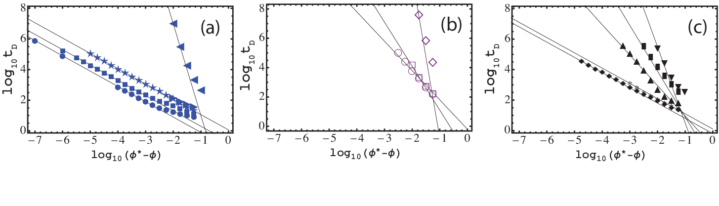
To verify the conceptual framework described in Sec. III, we performed microstate analyses for a variety of Q1D systems with different topologies and carried out extensive Monte Carlo simulations to measure the long-time diffusive relaxation time as a function of . A summary of our results is presented in Table 1 and Fig. 15. For systems denoted C–E in Table 1 we have performed a complete network analysis, and for the remaining cases the results are based on geometrical investigations of particle motion to identify bottleneck microstates.
Table 1 shows the number of compressed particles in the bottleneck microstates that were detected for a given system topology and indicates if a given microstate is untrapped (U), semitrapped (S), or trapped (T). The resulting crossing-frequency exponent is also given. Two examples of complete pathways that enable the particle labels of strings of particles to move forward or backward by one are depicted in Figs. 16 and 17 for systems D and E, respectively. The figures show displacements of individual particles that lead to each microstate transition. In addition, the compressed regions in the controlling bottleneck microstates are marked. In case D, the system goes through three types of bottleneck microstates: (a) a microstate with a one-particle trapped CR, (b) a microstate with a two-particle semitrapped CR, and (c) a microstate with a three-particle untrapped CR. All of these microstates yield the same crossing-frequency exponent for this topology. In case E, the evolution of the system is dominated by bottleneck microstates with all eight particles forming the compressed region. Since the bottleneck microstates are untrapped, we have for this topology.
The scaling behavior of the long-time structural relaxation time predicted by our bottleneck microstate analysis is compared in Fig. 15 with results of direct Monte Carlo simulations of the system. In all cases, we find that the simulation results are consistent with the results of our theoretical analyses. (We note, however, that due to extremely long simulation times required to determine the critical dynamics near KA, in not all cases the simulations allow a unique determination of the critical exponent.)


V Conclusions and Future Work
In this manuscript, we analyzed and performed Monte Carlo simulations of a quasi-one-dimensional model in which hard rods undergo single-file Brownian motion inside a series of intersecting narrow channels. Like supercooled liquids and glasses, this Q1D model displays slow and cooperative dynamics as the packing fraction approaches , which signals complete kinetic arrest and varies with the system topology. We provided a complete analysis of the model dynamics for several different topologies beyond the ‘figure-8’ model described previously [29].
We mapped each configuration of particles to a set of discrete microstates that describe the number of particles in each lobe and occupancy of the intersections. For several system topologies, we enumerated all microstates near and constructed directed graphs that identify all transitions between microstates. We find that Q1D systems must pass through a set of rare ‘bottleneck’ microstates to reach the long-time diffusive regime. The time required to reach the diffusive regime grows as a power-law, , as the packing fraction approaches with an exponent that is determined by the system topology. Note that since the packing fraction of kinetic arrest and the associated structural relaxation time can be calculated exactly, it is straightforward to fully equilibrate the system at each packing fraction.
We have identified several intriguing features of the dynamics of Q1D systems that require further investigation. First, our current studies have been limited to rather small numbers of particles and junctions . As shown in Fig. 4 (b), for small and , one is not able to obtain single-file diffusive behavior , with over a wide dynamical range.
To illustrate subdiffusive behavior in Q1D systems beyond the figure-8 topology, we carried out preliminary studies of the MSD for a system with , , and in Fig. 18. Even though the packing fraction in Fig. 18 is significantly below , we observe multiple plateaus and regions of subdiffusive behavior. The exponents of the subdiffusive behavior in regions c and e are approximately and , respectively. The slope of indicates possible single-file diffusive behavior [42, 43]. In future studies, we will investigate systems with increasing numbers of particles at fixed topology to test the robustness of the subdiffusive behavior, and identify rare microstates that give rise to structural relaxation from the caged regions b and d. These preliminary results indicate that there is nontrivial dynamics in Q1D systems even far from kinetic arrest.
We believe that this work will encourage new simulations and experiments of dense colloidal and other glassy systems in narrow channels and also in bulk to determine whether bulk systems can display quasi-one-dimensional dynamical behavior and whether the effective Q1D topology of the system can vary significantly with packing fraction.
Acknowledgments
Financial support from the NSF CBET-1059745 (J.B.) and DMR-1006537 (C.O. and P.P.) is gratefully acknowledged. This work also benefited from the facilities and staff of the Yale University Faculty of Arts and Sciences High Performance Computing Center and the NSF (Grant No. CNS-0821132) that in part funded acquisition of the computational facilities.
References
- [1] M. D. Ediger, C. A. Angell, and S. R. Nagel, “Supercooled liquids and glasses,” J. Phys. Chem., vol. 100, p. 13200, 1996.
- [2] A. Onuki, Phase Transition Dynamics. Chambridge University Press, 1st ed., 2002.
- [3] P. M. Chaikin and T. C. Lubensky, Principles of condensed matter physics. Chambridge University Press, 1st ed., 2000.
- [4] C. Angell, K. Ngai, G. McKenna, P. McMillan, and S. Martin, “Relaxation in glass forming liquids and amorphous solids,” J. Appl. Phys, vol. 88, pp. 3113–3157, 2000.
- [5] P. G. Debenedetti and F. H. Stillinger, “Supercooled liquids and the glass transition,” Science, vol. 410, p. 259, 2001.
- [6] C. S. O’Hern, L. E. Silbert, A. J. Liu, and S. R. Nagel, “Jamming at zero temperature and zero applied stress: The epitome of disorder,” Phys. Rev. E, vol. 68, p. 011306, 2003.
- [7] G. Marty, G. Marty, and G. Biroli, “Dynamical heterogeneity close to the jamming transition in a sheared granular material,” Phys. Rev. Lett., vol. 95, p. 265701, 2005.
- [8] R. Candelier, O. Dauchot, and G. Biroli, “The building blocks of dynamical heterogeneities in dense granular media,” Phys. Rev. Lett., vol. 102, p. 088001, 2009.
- [9] G. Marty and O. Dauchot, “Subdiffusion and cage effect in a sheared granular materials,” Phys. Rev. Lett., vol. 94, p. 015701, 2005.
- [10] P. N. Pusey and W. Van-Megan, “Observation of a glass transition in suspensions of spherical colloidal particles,” Phys. Rev. Lett., vol. 59, p. 2083, 1987.
- [11] J. G. Berryman, “Random close packing of hard spheres and disks,” Phys. Rev. A, vol. 27, p. 1053, 1983.
- [12] Random close packing for these systems are and for and polydispersities, respectively.
- [13] M. Tokuyama and Y. Terada, “Slow dynamics and re-entrant melting in a poly-disperse hard-sphere fluid,” J. Phys. Chem. B, vol. 109, p. 21357, 2005.
- [14] L. Angelani and G. Foffi, “Configurational entropy of hard spheres,” J. Phys.: Cond. Mat., vol. 100, p. 256207, 2007.
- [15] B. Doliwa and A. Heuer, “Cooperativity and spatial correlations near the glass transition: Computer simulation results for hard spheres and disks,” Phys. Rev. E, vol. 61, p. 6898, 2000.
- [16] E. Zaccarelli, C. Valeriani, E. Sanz, W. C. K. Poon, M. E. Cates, and P. N. Pusey, “Crystallization of hard-sphere glasses,” Phys. Rev. Lett., vol. 103, p. 135704, 2009.
- [17] Z. D. Cheng, P. M. Chaikin, S. Phan, and W. B. Russel, “Nature of the divergence in low shear viscosity of colloidal hard-sphere dispersions,” Phys. Rev. E, vol. 65, p. 041405, 2002.
- [18] D. Kaya, N. L. Green, C. E. Maloney, and M. F. Islam, “Normal modes and density of states of disordered colloidal solids,” Science, vol. 329, pp. 656–658, 2010.
- [19] S. R. Elliott, Physics of Amorphous Materials. Longman, 2nd ed., 1990.
- [20] E. G. D. Cohen and I. M. D. Schepper, “Note on transport processes in dense colloidal suspensions,” J. Stat. Phys., vol. 63, p. 241, 1991.
- [21] J. C. Dyre, “Colloquium: The glass transition and elastic models of glass-forming liquids,” Rev. Mod. Phys., vol. 78, pp. 953–972, 2006.
- [22] W. Van-Megan and S. M. Underwood, “Glass transition in colloidal hard spheres: Measurements and mode-coupling-theory analysis of the coherent intermediate scattering function,” Phys. Rev. E., vol. 49, pp. 4206–4220., 1994.
- [23] Y. Jung, J. P. Garrahan, and C. D., “Dynamical exchanges in facilitated models of supercooled liquids,” J. Chem. Phys., vol. 123, p. 084509, 2005.
- [24] C. Toninelli, G. Biroli, and D. S. Fisher, “Spatial structures and dynamics of kinetically constrained models for glasses,” Phys. Rev. Lett., vol. 92, p. 185504, 2004.
- [25] C. Toninelli, G. Biroli, and D. S. Fisher, “Jamming percolation and glass transition in lattice models,” Phys. Rev. Lett., vol. 96, p. 035702, 2006.
- [26] D. C. Viehman and K. S. Schwizer, “Theory of gelation, vitrification, and activated barrier hopping in mixtures of hard and sticky spheres,” J. Chem. Phys., vol. 128, p. 084509, 2008.
- [27] E. R. Weeks and D. A. Weitz, “Properties of cage rearrangements observed near the colloidal glass transition,” Phys. Rev. Lett., vol. 89, p. 095704, 2002.
- [28] E. R. Weeks, J. C. Crocker, A. C. Levitt, A. Schofield, and D. A. Weitz, “Three-dimensional direct imaging of structural relaxation near the colloidal glass transition,” Science, vol. 287, p. 627, 2000.
- [29] P. Pal, C. S. O’Hern, J. Blawzdziewicz, E. R. Dufresne, and R. Stinchcombe, “Minimal model for kinetic arrest,” Phys. Rev. E, vol. 78, p. 011111, 2008.
- [30] C. Donati, J. F. Douglas, W. S. Kob, J. Plimpton, P. H. Poole, and S. C. Glotzer, “Stringlike cooperative motion in a supercooled liquid,” Phys. Rev. Lett., vol. 80, p. 2338, 1998.
- [31] Y. Gebremichael, M. I. Vogel, and S. C. Glotzer, “Particle dynamics and the development of string-like motion in a simulated monoatomic supercooled liquid,” J. Chem. Phys., vol. 120, p. 4415, 2004.
- [32] K. Hahn, J. Kärger, and V. Kukla, “Single-file diffusion observation,” Phys. Rev. Lett., vol. 76, p. 2762, 1996.
- [33] C. Lutz, M. Kollmann, and C. Bechinger, “Single-file diffusion of colloids in one-dimensional channels,” Phys. Rev. Lett., vol. 93, p. 026001, 2004.
- [34] W. M. Chen and G. E. Uhlenbeck, “On the theory of brownian motion II,” Rev. Mod. Phys., vol. 17, p. 323, 1945.
- [35] R. Y. Rubinstein and D. P. Kroese, Simulation and the Monte Carlo Method. Wiley-Interscience, 2nd ed., 2007.
- [36] M. H. Kalos and P. A. Whitlock, Monte Carlo Methods. Willey-Interscience, 1st ed., 1986.
- [37] D. Frenkel and S. Berend, Understanding Molecular Simulation. Academic Press, 2nd ed., 2001.
- [38] W. H. Press, S. A. Teukolsky, and W. T. Vetterling, Numerical Recipes in C: The Art of Scientific Computing. Cambridge University Press, 2nd ed., 1992.
- [39] Deitel and Deitel, C++ How to Program. Prentice Hall, 5th ed., 2005.
- [40] J. G. Siek, L.-Q. Lee, and A. Lumsdaine, The Boost Graph Library: User Guide and Reference Manual. Addison-Wesley, 1st ed., 2002.
- [41] A. C. Telea, Data visualization: principles and practice. A K Peters, Ltd, 1st ed., 2008.
- [42] K. Nelissen, V. R. Misko, and F. M. Peeters, “Single-file diffusion of interacting particles in a one-dimensional channel,” Europhys. Lett., vol. 80, p. 56004, 2007.
- [43] A. Ryabov, “Single-file diffusion in an interval: First passage properties,” J. Chem. Phys., vol. 138, p. 154104, 2013.