Second order statistics characterization of Hawkes processes
and non-parametric estimation
Abstract
We show that the jumps correlation matrix of a multivariate Hawkes process is related to the Hawkes kernel matrix through a system of Wiener-Hopf integral equations. A Wiener-Hopf argument allows one to prove that this system (in which the kernel matrix is the unknown) possesses a unique causal solution and consequently that the second-order properties fully characterize a Hawkes process. The numerical inversion of this system of integral equations allows us to propose a fast and efficient method, which main principles were initially sketched in [1], to perform a non-parametric estimation of the Hawkes kernel matrix. In this paper, we perform a systematic study of this non-parametric estimation procedure in the general framework of marked Hawkes processes. We describe precisely this procedure step by step. We discuss the estimation error and explain how the values for the main parameters should be chosen. Various numerical examples are given in order to illustrate the broad possibilities of this estimation procedure ranging from 1-dimensional (power-law or non positive kernels) up to 3-dimensional (circular dependence) processes. A comparison to other non-parametric estimation procedures is made. Applications to high frequency trading events in financial markets and to earthquakes occurrence dynamics are finally considered.
Index Terms:
Stochastic processes Covariance matrices Estimation Microstructure Earthquakes Inverse problems Discrete-event systems Multivariate point processesI Introduction
A (multivariate) Hawkes process is a counting process which intensity, at each time, is given by a linear regression over past jumps of the process [2, 3]. This “self-” and “mutually-” exciting nature of Hawkes processes makes them very appealing to account, within a simple tractable model, for situations where the likelihood of future events directly depends on the occurrence of past events. For this reason, there has been, during last decade, a growing interest for Hawkes processes in various fields where endogenous triggering, contagion, cross-excitation can be naturally invoked to explain discrete events dynamics. Originally Hawkes models have been introduced to describe the occurrence of earthquakes in some given region [4, 5], but they also became popular in many other areas like high-frequency finance (trading and order book events dynamics) [6, 7, 8], neurobiology (neurons activity) [9], sociology (spread of terrorist activity) [10, 11] or processes on the internet (viral diffusion across social networks) [12, 13].
A -dimensional Hawkes process is mainly characterized by its kernel matrix , where the kernel describes how events of the th process component influence the occurrence intensity of the th component. As far as estimation of Hawkes process is concerned, in most studies, one assumes a specific parametric shape for the kernel components (e.g. an exponential decay) and performs either a moment method (based e.g. on the bartlett spectrum [14, 15]) or a maximum likelihood estimation [16, 17]. However, when one has no a priori on the shape of the kernel components, it is necessary to perform a non-parametric estimation. The first approach devoted to this goal was a method based on Expected Maximization (EM) procedure of a (penalized) likelihood function [18, 10]. It has been designed for monovariate Hawkes processes and can be hardly used to handle large amounts of data in situations where the kernel function is not well localized as compared to the exogenous inter-events time (see section VI). Another approach, proposed in [19, 20, 9], consists in minimizing a contrast function, assuming that the kernels can be decomposed over atoms of some dictionary. The estimation is regularized using a Lasso penalization which provides sparse estimations. The so-obtained kernels are, for instance, piece-wise constant functions with very few non zero pieces. Though it is clearly the right choice when the dimension is large or when the kernels are known to be very well localized (this seems to be the case when modeling networks of neurons [9]), it does not make sense when modeling earthquakes or financial time-series for which a large amount of data is available and the kernels are known to be power-law. Let us also mention an approach proposed in [21], where the authors estimate the kernel components from the jumps correlation matrix through a spectral method. This technique is however exclusively adapted to symmetric Hawkes processes.
In this paper, our main purpose is two-fold: We first provide a complete overview of Hawkes processes second order properties and show that they uniquely characterize the process, i.e., there is a one-to-one correspondence between the matrix and a matrix associated with the jumps () correlation function. In fact, we prove that is the unique causal solution of a system of Wiener-Hopf equations that directly involves the correlation function. We then show that this property allows us to propose a new simple non-parametric estimation method based on the explicit resolution of the Wiener-Hopf system using a Gaussian quadrature method. In many applications, it is interesting to consider a marked version of Hawkes processes, where the conditional intensities of the Hawkes components may also depend on some random variables (the marks) associated with each event through a matrix of mark functions. We write the new system of equations which links with the correlation function which is no longer a Wiener-Hopf system. In the case the mark functions are piecewise constant, we show that a simple variant of our method allows one to solve this system, i.e., to recover both the kernel and the mark functions matrices. We provide various numerical examples ranging from a 1-dimensional process up to a 3-dimensional process. We also provide some heuristics about the estimation error and convergence issues as well as some procedures to fix the various parameters of the method. We compare this method to existing non-parametric methods and show that it is relatively simple to implement and allows one to handle very large data sets and lead to reliable results in a wide number of situations. Our estimation framework is then illustrated on two different applications: First, along the same line as in Refs. [21, 22], we study the arrival of market orders of 2 liquid future assets on the EUREX exchange. We show that the estimated kernel is strikingly well fitted by a power-law function with an exponent very close to . Second, we estimate a Hawkes model of earthquake events marked by the event magnitudes from the Northern California EarthQuake Catalog (NCEC) [23]. To our knowledge, the only attempt to estimate a non-parametric self-exciting from earthquakes was provided in Ref. [18]. In our case we confirm that the ETAS model specifications, i.e. of power-law shape of the kernel and an exponential law for the mark function.
The paper is structured as follows: In section II, we introduce the main mathematical definitions and review the second order properties of multivariate Hawkes processes. We notably provide the explicit expression for the Laplace transform of the jump correlation function. We also introduce the conditional expectation matrix and show how it is basically related to the jump correlation function. Finally, we recover a former result by Hawkes [3] by virtue of which the kernel matrix satisfies a Wiener-Hopf equation with as a Wiener-Hopf kernel. We show that the Wiener-Hopf operator has a unique causal solution and thus is uniquely determined by the shape of . Our estimation method relies on this property and is described in section III. More precisely, by reformulating a marked Hawkes process with piecewise constant mark functions as a multivariate Hawkes process in higher dimension, we propose a numerical method that allows one to estimate both the kernel and the mark functions. This method mainly uses a Nyström method to solve the system of Wiener-Hopf equations. It is illustrated in Section V on four different examples : a 2-dimensional marked process, two 1-dimensional processes (one involving slowly decreasing kernels and one involving a negative-valued kernel) and a 3-dimensional process (involving circular dependance and non decreasing kernels). Section IV presents some heuristics about the analysis of the estimation errors and discusses some procedures to fix the main parameters of the method (namely, the bandwidth and the number of quadrature points). We then briefly discuss the link to former approaches for non-parametric kernel estimation in section VI, while the aforementioned applications to financial statistics and geophysics are considered in section VII. Conclusion and prospect are given is section VIII.
II Multivariate Hawkes Processes and their second order properties
II-A The framework
We consider a -dimensional point process . Each component is a 1d point process whose jumps are all of size 1, and whose intensity at time is . Thus the intensity vector of is .
We consider that is a Hawkes process [2], i.e., that, at time , each intensity component can be written as a linear combination of past jumps of , i.e.,
| (1) |
where
- •
are exogenous intensities
- •
each kernel function is a positive and causal (i.e., its support is included in ). It codes the influence of the past jumps of on the current intensity . In the following, the kernel matrix will denote the matrix function .
Using matrix notations, the equations (1) can be rewritten in a very synthetic way as
| (2) |
where and the operator stands for regular matrix multiplications where all the multiplications are replaced by convolutions.
Let us remind that the process has asymptotically stationary increments (and the process is asymptotically stationary) if the following hypothesis holds [2] :
- (H)
the matrix has a spectral radius strictly smaller than 1,
where stands for . In the following we will always consider that (H) holds and we shall consider that corresponds to the asymptotic limit, i.e., has stationary increments and is a stationary process.
In that case, the vector of mean event rates associated with each component reads [2]:
| (3) |
In the following, will refer to the th component of .
Remark (Inhibitory effects in Hawkes processes).
Let us point out that Brémaud and Massoulié [24] have shown that the stability condition criterium remains valid when is a nonlinear positive Lipschitz function of and where the kernels are not restricted to be positive. A particular interesting generalization of Eq. (2) (notably considered in [20]) is:
| (4) |
where if and otherwise. This extension allows one to account for inhibitory effects when can take negative values.
II-B Characterization of a multivariate Hawkes process through its second-order statistics
In this section we recall the main properties of the correlation matrix function associated with multivariate Hawkes processes and prove that it fully characterizes these processes.
The second-order statistics are summed up by the infinitesimal covariances :
| (5) |
As already explained, under assumption (H), can be considered to have stationary increments, consequently, only depends on . Moreover, these measures are non singular measures, except for for which it has a Dirac component . Thus the non-singular part of this covariance can be written as
| (6) |
where is the Kronecker symbol which is always 0 except when in which case it is equal to 1.
Let us point out that, since all the jumps of the process are of size 1, the second order statistics can be rewritten in terms of conditional expectations (see [1]). Indeed, for all , let be the non-singular part of the density of the measure , i.e.,
| (7) |
Then
It follows that:
| (8) |
where stands for the transpose of the matrix .
In [21], it has been shown that the ”infinitesimal” covariance matrix can be directly related to the kernel matrix :
Proposition 1 (from [21]).
Let , where stands for the matrix convolution (where is repeated times). Let . Then
| (9) |
where is the diagonal matrix defined by and where we use the convention . In the Laplace domain, this last equation writes
| (10) |
Moreover,
| (11) |
where the Laplace transform of a causal function is defined as:
| (12) |
From Eqs (8) and (9), it results:
| (13) |
or alternatively, in the Laplace domain
| (14) |
Since
| (15) |
convoluting both hand sides of (13) by leads to
| (16) |
which gives
| (17) |
Since all the elements of are causal functions (i.e., supported by ) and since is just expressed as convolution products of the matrix , all the elements of are also causal functions. Writing this last equation for , thus leads to the following Proposition:
Proposition 2.
The kernel matrix functions statisfies the -dimensional Wiener-Hopf system
| (18) |
Wiener-Hopf equations have been extensively studied in the past century [25, 26, 27] and arise in wide variety of problems in physics. This last system of equation was first established by Hawkes in [3] (see also [1]) in order to express (considered as the ”unknown”) as a function of . He proved that it has a unique solution in . One can work the other way around and consider it as a system of equations that (the ”unknown”) satisfies, being known. In Appendix A, thanks to the famous factorization technique introduced by Wiener and Hopf [27], we prove that this system (18) admits a unique solution in :
Theorem 1.
Let be a -dimensional Hawkes process with exogenous intensity and kernel matrix as defined in Section II-A. Let satisfies hypothesis (H) (as explained above, we then can consider that has stationary increments). Let be the matrix defined by (7). Then the matrix is the only solution (whose elements are all causal and in ) of the system of equations (in which is the unknown)
| (19) |
One can then state the corollary :
Corollary 1.
III Non-parametric estimation of a multi-dimensional marked Hawkes process : framework and main principles
As we shall see at the end of this Section, the results of previous Section naturally lead to a non-parametric estimation method for multidimensional Hawkes processes. Actually, we shall develop our estimation framework in a slightly more general framework than the one presented above which is very useful in applications : the framework of multi-dimensional marked Hawkes process.
III-A The marked Hawkes process framework
Using the same notation as in Section II-A, each component is now associated with observable iid marks . is non zero only at time when jumps. In the following, we note the density of the law of the random variable conditionally to the fact jumps. We then replace (1) by the new equation
| (20) |
where the past observed marks influence the current intensity through the unobserved mark (positive) function . Since is only involved through the product , it is defined up to a multiplication factor. We fix this factor by choosing such that .
As in the unmarked case, it is easy to show that under the condition (H), one can consider that has stationary increments and that (3) still holds.
In place of the functions for an non-marked Hawkes process (see (7)), we now define the function as
| (21) |
Let us note that . In Appendix B we prove that satisfies a system of integral equation as stated by the following proposition:
Proposition 3.
Let fixed. The kernels of the marked Hawkes process defined in Section III-A satisfy the following system of integral equations :
| (22) |
where
| (23) |
III-B The Wiener-Hopf equation in the case of piece-wise constant mark functions
In a non-parametric estimation framework, the unknown of the system (22) are both the kernels and the mark functions . In the case of non-marked Hawkes process, we already showed (see Eq. (18)) that this system is a Wiener-Hopf system. We proved the unicity of the solution and, one can use standard methods for solving it. The system (22) is no longer a Wiener-Hopf system which makes things much harder.
In the particular case of piece-wise constant mark functions (with number of pieces), it is easy to prove that the process basically corresponds to a non-marked Hawkes process of dimension : each components corresponds to the jumps of a component of the marked Hawkes process associated with one of the mark function values. Thus it is clear that the system (22) can be written in terms of a Wiener-Hopf system of the type of (18). It will be the base of our non-parametric estimation procedure.
Remark : Before moving on, let us point out that, in the case the marks influence the intensity of the process only through a finite number of values, one could consider the more general framework where the kernels themselves depend on the marks, i.e.,
| (24) |
and, following the same argument as above, estimate all the kernels solving a Wiener-Hopf system. This can be achieved following the exact same lines as the algorithm described in the next Section. For the sake of simplicity, we will describe the algorithm in the case .
We consider that for any , there exists a covering of with a finite number of intervals such that, for any and for any , restricted to is a constant function which value is :
| (25) |
Since the marks are involved in the process construction only through the functions , it is clear that the functions are also piece-wise constant. Thus we note
| (26) |
In the same way, we note
| (27) |
For fixed and , and for a fixed , Equations (22) and (23) then rewrite
| (28) |
Since, , one has , then, if we make the change of variable (consequently ), we get
| (29) |
We finally get the Wiener-Hopf system
Proposition 4.
Let fixed. The marked kernels satisfy the following Wiener-Hopf system :
| (30) |
where
| (31) |
Moroever,
| (32) |
Thus we get Wiener-Hopf systems of dimension where . The unicity of the solution is actually deduced from the result of Section A where we proved the unicity of the solution of the system (18). Indeed, as we explained in the previous Section, the marked Hawkes process we considered here is equivalent to a non-marked Hawkes process of dimension .
Let us point out that, in the case the functions are constant functions (and thus equal to 1, since ), then we recover the system (18) (which corresponds to Wiener-Hopf systems of dimension ). Indeed, in that case we have , , and, for all , .
III-C Discretizing the system (22) using Nyström method
Solving the Wiener-Hopf systems (30) is the main principle of our estimation procedure. There is a huge literature about numerical algorithm for solving Wiener-Hopf equations [27, 28]. One algorithm which is particularly simple and which works particularly well is the Nyström method[29]. It basically consists in replacing convolutions (in time) by discrete sums using quadrature method with points. Then, for each , solving (30) amounts in solving a linear dimensional standard linear system which can be solved by simply inverting the corresponding matrix. Of course, in order to get the full estimation of the kernels and the constants , one has to solve such systems (one for each value of ). Let us point out that, when the kernels have been estimated on the quadrature points, using quadrature formula, one can compute these estimations on any finer grid.
If we suppose that the kernels are supported by one gets
| (33) |
However, when using the Nyström method, i.e., computing the integral using quadrature methods, one has to be careful since the kernel is generally discontinuous at . A standard way to deal with a Wiener-Hopf kernel which is singular (non exploding) on the diagonal, is to rewrite (33) in the following way :
| (34) |
The term in the first integral is then no-longer discontinuous (quadrature error will be one order smaller) and the second term can be estimated directly, estimating directly the primitive function of the functions and using the formula
| (35) |
III-D Main steps od our non-parametric estimation
We are now ready to present the main steps of our estimation algorithm. We refer the reader to Section V-A for a more detailed description of the algorithm. The main steps for non-parametric estimation of multi-dimensional Hawkes processes are :
- •
For all , fix a priori the intervals on which the mark function is considered as constant.
- •
For all and , estimate the conditional-law functions as defined by (21) by replacing the expectation by empirical averages. These functions are are density measures, in particular they are positive (cf (13)) though they do not sum to 1. It is very natural to use classical kernel-based non-parametric estimation techniques used for estimating the density of a random variable from iid realizations [30]. This classically involves a bandwidth parameter which corresponds to the size of the support of the kernel. This well be developed in the Section IV-A.
- •
- •
Using quadrature formula, the so-obtained estimation of (at the quadrature points) can be re-sampled on any grid with an arbitrary resolution.
This method mainly involves two key parameters : the bandwidth and the number of quadrature points. The next section gives some insights on how one should fix these two parameters.
IV Selection of the bandwith and the number of quadrature points
The goal of this Section is to give qualitative arguments for controlling the error of the estimation procedure presented previously and to understand how to choose the estimation parameters (the bandwidth) and (the number of quadrature points). It will be illustrated by numerical simulations.
For the sake of simplicity, we shall consider that the Hawkes process is not marked. The arguments are exactly the same in the case of a marked Hawkes process.
There are mainly two sources of errors :
- ()
the first one comes from the estimation of the conditional expectation density (7). This error is basically controlled by the amount of data available, i.e., by the number of jumps available, and by the value of the bandwidth parameter .
- ()
The other one comes from the inversion of the Wiener-Hopf system (18). This error is basically controlled by the number of quadrature points.
In the error analysis, it is very hard to take into account the fact that the kernel of the Wiener-Hopf system is a random function (i.e., the empirical estimation of the conditional expectation). This problem has somewhat already been addressed in [20] in a particular case (see Section VI). Clearly, this problem should be solved for understanding deeply the performance of our estimator. However, in the general case, this is a very difficult problem which is still open as of today.
IV-A Conditional expectation density estimation - Bandwidth () selection
One of the main step of the algorithm presented in Section III-D consists in estimating the functions 11 1 In the non marked case the functions are such that , defined by (7), for (for negative , one can use the formula ).
These functions are density measures, in particular they are positive (cf (13)) though they do not sum to 1. It is very natural to use classical kernel-based non-parametric estimation techniques used for estimating the density of a random variable from iid realizations [30].
Let be a kernel function of order , i.e., a localized function such that , and for all , . Since we want to perform estimations only for , it is convenient to choose the support of to be in . For the sake of simplicity, we consider that we have iid realizations of the Hawkes process on an interval (such that ). For each realization , we call the th jumping time of the th component . For a given bandwidth , it is natural to consider the following estimator of for
| (36) |
The mean square error is defined as:
where we denoted the estimation bias . The following classical bound of this error is proven in Appendix C:
Proposition 5 (Convergence speed).
If is Hölder and if the kernel is of order , then mean square error (MSE) satisfies
| (37) |
The minimum is obtained for22 2 Notice that, the minimum depends on and but we chose to omit the superscripts for the sake of simplicity.
| (38) |
for which one gets the usual adaptive non-parametric convergence speed
| (39) |
Thus, for instance, in the special case where the ’s are Hölder 1 (i.e., ), using a simple order 0 kernel (such as ), one gets that if one chooses of the order of , we expect the MSE to be of the order of where is the number of iid realizations of the Hawkes process. Let us point out that, in practice, one often has a single realization. One can then estimate by averaging on the different jumps of this realization. More precisely, we replace (36) which used realizations on the time interval by the following estimation that uses a single realization on the time interval (with ) :
| (40) |
where is the number of events of the realization. After a certain time, the realization can be considered as independent of its beginning. One should then get an error which is of the order of
| (41) |
so for that gives an error of the order of .
These results are illustrated in Fig. 1 where we have computed the integrated MSE (MISE) on in a 1-dimensional Hawkes model with an exponential kernel (, ) for different realization sizes increasing from to by a factor 2. In order to estimate the MISE, for each parameter, we have generated 500 trials of the model and estimated the MISE using the analytical expression of . One can see in the log-log representation, that for each sample size (), the error decreases in the small regime as expected from Eq. (72) as . For large values of , one clearly observes the bias contribution that is expected to behave like . We have checked that the optimum value () behaves for large as . In the right panel figure is reported, in log-log scale, the minimum MISE error as a function of the sample size. As predicted by Eq. (39), one gets a power-law with an exponent close to .


Bandwdith selection using cross-validation. From a practical point of view, in order to choose the optimal value of the bandwidth from a single realization () on the time interval , one can use a cross-validation method. Indeed, in the MISE computation, the only terms that depend on read:
| (42) | |||||
where we have considered that has a support included in and where we used the definition . Replacing the last term in the expectation of the previous equation by an empirical average, it results that the following contrast function provides an (unbiased) estimator of :
| (43) |
where stands for the number of events of , the first sum is taken on all the jumping times of the component and the second sum is taken on all the jumping times of the component such that . A cross-validation method can be used to estimate the expectation of . For doing so, one divides the overall realization time interval in intervals of equal size, i.e., for . Then, for each interval , the conditional expectation is estimated following the same ideas as (40), averaging only on the jumps of which do not take place in . More precisely, we get the estimation defined by
| (44) |
where corresponds to the number of jumps of that take place in the time-interval . The contrast function (43) is then estimated on , i.e.,
| (45) |
The estimation of is thus naturally given by averaging on all the so-obtained quantities for all the possible choices of :
| (46) |
Examples of curves are provided in Fig. 2 on a simple 1-d example of Hawkes process. The estimation is close the theoretical quantity . The abscissa corresponding to the minimum of the so-obtained curve gives an estimation of the optimal bandwidth
IV-B Overall error - Selection of the number of quadrature points
If one supposes that is estimated with no error, it remains to study the error due to the quadrature approximation. The function is the kernel of the Wiener-Hopf system (18). Even if the functions are regular, this is a singular kernel since it is generally discontinuous on its diagonal (except if the dimension ). There is a huge literature on how to solve numerically Wiener-Hopf systems with a singular kernel on its diagonal (though generally the singularity is much stronger than a ”simple” discontinuity). It is out of the scope of this paper to compare all these methods and try to understand which is more appropriate for our estimator. A pretty popular method is the Nyström method already described above. It consists in rewriting (18) as we did when we rewrote (33) into (34), i.e., isolating the singular behavior of the kernel:
The last integral term can be estimated ”directly”, i.e., estimating the primitive function of . The other integral term is approximated by a quadrature method (we shall use Gaussian quadrature).
Let us suppose again that each element of is Hölder (we assume here that ) and that they are all bounded by a constant . Again using (13) and (71), one can easily show that each element of is bounded by : , where and are some constants. Let us also suppose that all the elements of the derivative are bounded by a constant . Then, the terms in are of class Hölder everywhere, except on the diagonal for which the derivative might be discontinuous. If the quadrature method uses points and is basically of order greater than , the error for the non diagonal terms is of the order of while the error on the diagonal terms is of the order of . The total quadrature error is of the order of
Solving the Wiener-Hopf equation amounts in applying the convolution operator whose Laplace transform is (see (14))
This operator has a norm which is bounded by a constant times . Thus the error resulting from the Wiener-Hopf inversion is of the order of the quadrature error :
| (47) |

.
Since, as we have just seen, the Wiener-Hopf inversion involves an operator whose norm is bounded by a constant (controlled by ) the Wiener-Hopf kernel estimation error (related to to error in the estimation of ) does not change of magnitude order when inversion is performed. We deduce that the order of the overall error (when ) should basically be of the order of the sum of the two errors (see (41))
Again, as explained in the introduction of this section, we left apart the fact that the inversion of the system involves a random kernel that we need to control in order to control the error. In that respect, one can always choose large enough so that the quadrature error is negligible as compared to the estimation error () so that the overall error will always behave as .
In Fig. 3, we have reported the error on as a function of the sample size for the n-dimensional Hawkes process used previously. We set and chose, for each , (i.e. the optimal bandwidth). One can see that the error behaves as the the root mean square error (RMSE) on , i.e., as .

Selection of the number of Quadrature points . From a practical point of view, in order to choose the number of quadrature points that are used, one can start with a relatively small value for (e.g. ), compute the estimated kernels and compare them to the estimated kernels that are obtained when increasing the value of . One should stop increasing when the two estimations are “sufficiently close”. In order to decide whether is large enough, one can e.g. check if the relative variation,
| (48) |
is small enough (for instance ). This is illustrated in Fig. 4, where we have plotted, as a function of , both the relative estimation error and for 2 examples of 1D Hawkes processes involving respectively an exponential (top) and power-law kernel (bottom). One can see that in both situations, is large enough. For all the numerical illustrations and applications presented in this paper, a value in that range has been chosen. Empirically, we observed that, for a wide variety of kernels shapes and for sample sizes between and , this range is sufficient to be close to optimal results.

V Description of the algorithm - Numerical illustrations
The following section gives a detailed description of the algorithm and the next one gives several numerical illustrations.
V-A Description of the algorithm
In this Section, we describe precisely each step of our non-parametric estimation procedure within the framework of marked Hawkes processes presented in Section III.
- •
Estimation of the vector (simply using as an estimator of the number of jumps of the realization of divided by the overall time realization)
- •
For all , one must a priori choose and the intervals
- •
For all and for all , estimation of the probabilities as defined by (27). In order to do so, one just needs to count the number of realized marks that falls within the interval .
- •
One must estimate (on an a priori chosen support ) using empirical averages as explained in Section IV-A. For this purpose a value for the bandwidth must be chosen. Section IV-A explains (for the sake of clarity, this section only deals with the simpler case of non-marked Hawkes process, but the generalization is obvious) how this value can be obtained using cross-validation.
- •
Fix the number of quadrature points to be used as well as the support for all the kernel functions (we use gaussian quadrature). In general is sufficient, however, at the end of Section IV-B, we explain how this value can be chosen adaptively. Then, for each , solve the linear system obtained by discretizing the convolutions in (29) using the quadrature points. This leads to an estimation of all the functions on the quadrature points.
- •
The estimations of the kernels (on the quadrature points) are simply obtained using the formula . The norm as well as a re-sampling of the kernels on a high resolution grid can be obtained using again quadrature formula.
- •
The stability condition of the so-estimated Hawkes process should be checked (i.e., the spectral radius of the matrix made of the norms must be strictly smaller than 1).
- •
The estimation of the piece-wise values of the mark functions , can be obtained via the formula .
V-B Numerical illustrations


In this section, we illustrate the performances of the previous estimation method on various examples accounting for different situations: marked process, non decreasing lagged kernels, slowly decreasing kernels and kernels that can be negative.
In order to perform numerical simulations of -dimensional Hawkes models, various methods have been proposed. We chose to use a thinning algorithm (as proposed, e.g., in [31]). It is an incremental algorithm, the jumping times are generated one after the other. In its simplest version (in the case of decreasing kernels), at a given time , it basically consists in picking up the next potential jumping time using an exponentially distributed random variable with parameter . Then a uniform random variable on is drawn. If , the jump is rejected. If not rejected, it is assigned to the th component such that is the maximum index which satisfies .
A marked 2-dimensional Hawkes process with exponential kernels
The first example we consider is a 2-dimensional marked hawkes process
with exponential kernels. The matrix of the process reads:
with , . We consider that is marked with a mark that follows an exponential distribution of mean value . We choose the mark functions: and , i.e., the mark only impacts (linearly) the intensity of the process .
In Fig. 5 are reported the estimated kernels and mark functions obtained using a realization of this 2-dimensional process with 4.5 (resp. 4 ) events for component (resp. ). For the mark function estimation, we supposed that is piecewise constant on intervals for . One can see in the four top figures that each of the exponential kernels are well estimated (see the next section for a discussion of the error values). In the last two figures, we show that one also recovers the mark functions.
In the estimation procedure, we chose and (see Section IV for discussion on how to choose these values).
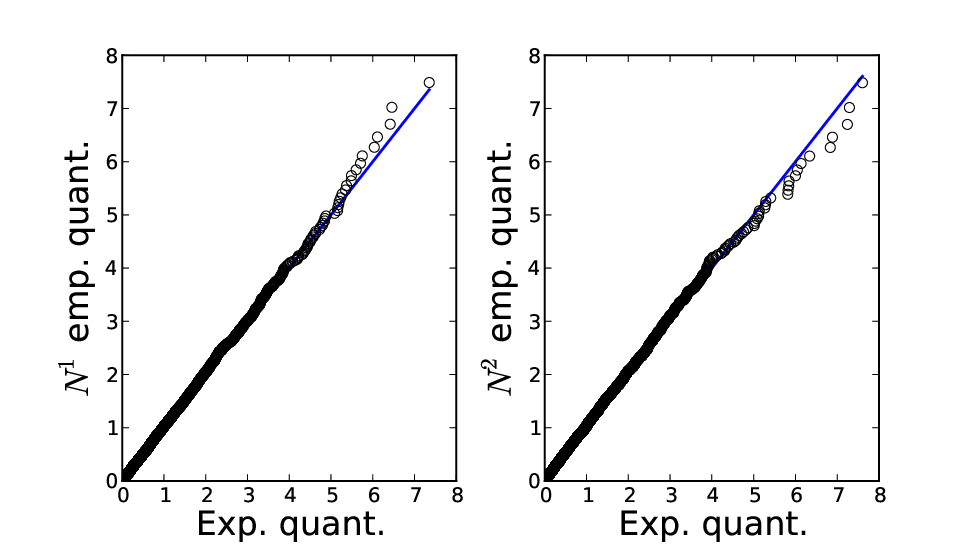
In order to check our estimation and test the Hawkes model on a set of data, one can perform a goodness-of-fit test by simply noting that each point process component, , considered as a function of a “time” , is an homogeneous Poisson process. In that respect the inter events times expressed in must be exponentially distributed, i.e., for each , if denote de jumping times of , then:
| (49) |
must be iid exponential random variables. From the estimated kernels, baseline intensities and mark functions, one can perform estimations of all the ’s. In Fig. 6 are displayed the Q-Q plots of the empirical quantiles distribution ( and were estimated from the last intervent times of each components) versus the exponential quantiles. One can check in both case that both curves are very close to the expected diagonal.
A three dimensional example with circular interactions
In this example, we aim at illustrating two features: first, one can faithfully estimate
Hawkes kernels that are not necessarily decreasing, localized around .
One can also, in a multidimensional Hawkes process, disentangle in the complex dynamics of the
events occurrence, the causality (in the sense of Granger causality) relationship between these events.
For that purpose we consider a 3-dimensional Hawkes process with “circular” interactions, i.e.,
the process is excited only by the processes itself excited by the process
which events are triggered by the events of .
Thus in the Hawkes matrix, only the terms , and are
non zero. We choose the shape of these kernels to be triangular functions with different positions.
In Fig. 7, we report the results of the estimation of such process on a sample
where each process has around events.
we can see that one remarkably recovers both the causality relationship between the 3 processes
and the triangular shapes of the interaction kernels.
Kernel with heavy tail
In Fig. 8, is reported the estimation of a 1D Hawkes model with
the power-law decreasing kernel with
and . Unlike the previous examples, this kernel has an algebraic
decay for large . One can see in both panels of Fig. 8 (corresponding
to linear and log-log representation) that, for a sample of events, our estimation is
very close to the expected kernel on a wide range to time scales. Let us notice that in order
to estimate a kernel that is slowly decaying over a support extending over several decades,
the regular sampling schemes of and is not suited since it would involve
an exponentially large matrix to invert. For that purpose, in ref. [32], we propose
a variant of the method of section III that relies on a different (i.e., logarithmic) time
sampling and that allows one to estimate when it varies
over a time interval of several orders of magnitude.
Kernel with non-positive values
The last example we provide, concerns a 1D Hawkes process that involves a kernel with negative values. Indeed, according the remark Remark, one can consider Hawkes processes with inhibitory
impact of past events (instead of exciting) when the kernel
takes some negative values. In that situation, if, in Eq. (4), the events corresponding to occur with a negligible probability, the model remains linear
and one can expect our estimation method to be still reliable. This is illustrated in Fig. 9 where
the estimation is performed using a sample (of events)
of a 1D Hawkes model with the kernel represented by the solid line: this kernel is either piecewise constant or piecewise linear and is negative on a whole interval before becoming positive.
According to this model, the occurrence of some event begins by decreasing the probability of occurrence
of further events while, after some time lag, this event has an
opposite impact and increases the process activity.
By comparing estimated and real kernel values, one can see that
even in that case, the method of section III provides provides
a fairly good estimation of the kernel shape.
VI Link with other approaches
In the academic literature, there are very few non parametric estimators of the kernel matrix of a Hawkes process. In the particular case the kernel matrix is known to be symmetric (which is always true if the dimension ), the method developed in [21] uses a spectral method for inverting (10) and deduces an estimation from the second-order statistics. It can be seen as a particularly elegant way of solving the Wiener-Hopf equation when the kernel is symmetric and in that respect, it is very similar to our approach (though not at all as general of course).
Apart from this method, there are essentially two other approaches for non parametric estimation.
The first one, initiated by [10], corresponds to a non parametric EM estimation algorithm. It is based on regularization (via penalization) of the method initially introduced by [18] in the framework of ETAS model for seismology (see Section VII-B for ETAS model). It has been developed for 1-dimensional Hawkes process. The maximum likelihood estimator is computed using an EM algorithm :
- •
The step basically corresponds to computing, for all and , the probability that the th jump has been ”initiated” 33 3 Here we refer to the ”branching” structure of the Hawkes process. by the th jump (where ), knowing an approximation of the kernel and of .
- •
And the step corresponds to estimating and knowing all the .
In [10], some numerical experiments on particular cases are performed successfully even when the exogenous intensity depends slowly on time : the whole function is estimated along with the kernel with a very good approximation. However, as emphasized in [10], the convergence speed of the EM algorithm drastically decreases when the decay of the kernel is getting slower (e.g., power-law decaying kernel). Equivalently, it also drastically decreases when one increases the average number of events that occur on an interval of the same size order as the one of the support of (keeping constant the overall number of events , i.e., shortening the overall realization time ). This can be performed, for instance, by simply increasing the baseline (keeping constant ).
This result is illustrated in Fig. 10, where we have compared, for a fixed estimation precision, the computation time of the EM method (without any regularization) and the computation time of our approach based on solving the Wiener-Hopf equation. All our tests are using a simple 1d Hawkes process with an exponential kernel. In a first experiment, we compared the ratio of the convergence times as a function of the overall number of events in the sample. As illustrated by the curve represented by symbols () in Fig. 10, we observed that, up to a logarithmic behavior, the computation times of both methods are comparable. In a second experiment (solid line curve in Fig. 10) we fixed the total number of jumps and let the number of events over the support of the kernel vary by simply changing the baseline intensity . In that case, one clearly observes that, as increases, the EM approach becomes slower as compared to our method.
A second important drawback of the EM approach is illustrated in the figure 11 where we have tested the EM algorithm on the example of Fig. 9 where the Hawkes process involves a kernel with negative values. While our method is able to handle inhibitory situations (provided the inhibitory effect does not leads to negative intensities), the probabilistic interpretation of the kernel values involved in the EM method, prevent any such possibility. One can see in Fig. 11 the EM method only allows one to estimate the positive part of .


In a recent series of papers [19, 20], some authors proposed, within a rigourous statistical framework, a second approach for non-parametric estimation. It relies on the minimization of the so-called contrast function. Given a realization of a Hawkes process (associated with the parameters ), on an interval , the estimation is based on minimizing the contrast function :
| (50) |
where
| (51) |
and
| (52) |
Let us point out that, minimizing the expectancy of the contrast function is equivalent to minimizing the error on the intensity process. Indeed, if is the information available up to time , since , one has
The minimum (zero) is of course uniquely reached for and . Since is expressed linearly in terms of and of the , minimizing the error is equivalent to solving a linear equation, which is nothing but the Wiener Hopf equation (18). Consequently, minimizing the expectancy of the contrast function is equivalent to solving the Wiener-Hopf equation.
In [20], the authors chose to decompose on a finite dimensional-space (in practice, the space of the constant piece-wise functions) and to solve directly the minimization problem (50) in that space. For that purpose, in order to regularize the solution (they are essentially working with some applications in mind for which only a small amount of data is available, and for which the kernels are known to be well localized), they chose to penalize the minimization with a Lasso term (which is well known to induce sparsity in the kernels), i.e., the norm of the components of . Let us point out, that minimizing the contrast function and minimizing the expectancy of the contrast function are two different stories. The contrast function is stochastic, and nothing guarantees that the associated linear equation is not ill-conditioned. In [20], the authors prove that, in the case
- (i)
the component of are picked up from an orthogonal family of functions, and
- (ii)
any two components of are always either equal or orthogonal one to each other,
then the linear equation is invertible, i.e., the associated random Gram matrix is almost surely positive definite. In applications (they study real signals from neurobiology [9]), they choose the components of to be piece-wise constant and give a lot of examples of the resulting estimations.
In the present work, our approach is quite different and is motivated for modeling large amount of data (e.g., earthquakes, financial time-series) which are well known to involve very regular non localized kernels. We directly solve the linear equation, i.e., the Wiener-Hopf system. In that case, we also introduce a regularization component by the mean of the choice of the quadrature method. Using a Gaussian quadrature with points, for instance, amounts in considering that the kernel term in the Wiener-Hopf equation is polynomial of order . Let us point out that though we proved that the Wiener-Hopf equation is invertible, we do not have any result on the invertibility of the stochastic version of the Wiener-Hopf equation in which the conditional expectations are replaced by empirical averages. As we will see in the next Sections, in all our applications and simulations, it does not seem to be a problem. This is clearly due to the fact that we always consider that a large amount of data is available (e.g., financial high frequency time-series, earthquake time-series). It seems that if a very small amount of data is available, both approaches described above should be more appropriate than our approach. For our approach to work, we would certainly need to add a regularization term for inverting the discrete linear system. This will be addressed in a future work.
VII Examples of application
VII-A Application to financial time-series

Because of their natural ability to account for self and mutual excitation dynamics of specific events, Hawkes processes have sparked an increasing interest in high frequency finance [6, 7, 8, 33, 21, 1, 22]. In this section, we consider, as a first application, a 1-dimensional Hawkes model for market order arrivals. The trading rate in financial markets has non trivial statistical features and is one the key factors that determines volatility. We use intraday data of most liquid maturity of EuroStoxx (FSXE) and EuroBund (FGBL) future contracts. Our data correspond to all trades at best bid/ask during 1000 trading days covering the period from may 2009 to september 2013. The number of events (market orders) per day is close to for FSXE and for FGBL. It is well known that market activity is not stationary and is characterized by a U-like shape. In order to circumvent this difficulty one can perform an estimation at a fixed time period within the day. However, as emphasized in [1], it appears that the kernel shape is constant for each period (the non-stationarity of the trade arrival rate can be associated with a varying baseline intensity ) and that estimating this kernel on each of these small periods and averaging on all the so-obtained estimations lead to the same estimation. This is why we did not consider the problem of intraday non-stationarity and performed the estimation over a whole trading day. In left Figure 12, we have reported the kernels of trades associated with FSXE and FGBL as estimated using the method described in section V-A (without considering any mark). The curves are displayed in log-log representation since both kernels are obviously very close to a power-law. They are well fitted by:
| (53) |
with and . In right Figure 12, we have reported the same estimation for FSXE market orders but with 4 different values of the sampling parameter (we chose seconds) in order to cover a wide range of times . One sees that all curves consistently fall on the analytical expression (53). This figure, where a scaling behavior of can be observed over a range of 5 decades, is very similar to the estimation performed by Bouchaud et al. on the S&P 500 mini [22]44 4 It is noteworthy that these authors found values of and that are consistent with the previous reported values.. Let us notice that origin of the power-law nature of Hawkes kernels for market data is a challenging question already raised in ref. [21, 1]. It is also remarkable that the shape of the kernel appears to be almost constant for different markets. Let us finally point out that in order to have , expression (53) must be truncated at both small and large time scales. This point is discussed in Refs. [21, 22]. However, it is important to notice that the expression (53) has to be integrated over 9 decades in order to reach (ie., if the minimum time resolution is s, even after one month, the integral of is still smaller than 1).
VII-B Application to earthquake time-series

Various point processes models have been proposed in order to reproduce the dynamics of seismic events (earthquakes) in some given geographic region (see e.g. [4, 34] for a review). Among theses models, the Epidemic Type Aftershock Sequence (ETAS) proposed by Ogata [35] is one of the most popular. This model accounts for the triggering of future events (aftershocks) by former earthquakes simply by assuming that the shocks dynamics corresponds to a Hawkes process marked by the events magnitude. More precisely, the one dimensional version of this model 55 5 There exists a space-time version of the ETAS model that accounts for both the time and the location of earthquakes. is defined as follows: is the baseline intensity, the kernel is
| (54) |
while the mark function (the “productivity law”) has an exponential like form:
| (55) |
Notice that the probability distribution of earthquake magnitudes is given by the famous Gutenberg-Richer law according to which the probability that an earthquake magnitude is greater than (large enough, i.e., greater than a given threshold ) reads
| (56) |

In Fig. 13, we have displayed as a function of where is the number of events of magnitude as estimated from data of the Northern California Earthquake Catalog [23] (NCEC). This catalog contains events of magnitude in the region of Northern California from january 1990 to october 2013. The total number of events is around . One can check that the Guttenberg-Richter law (56) provides a good fit of the data. Notice that despite the large number of studies devoted to ETAS model application to earthquake data (see e.g. [4, 34]), to our knowledge, only ref. [18] performed a non parametric estimate within the general class of linear self-exciting point processes. As previously mentioned (see section VI) these authors obtained an estimation of the kernel shape by applying an Expected Maximization iterative method. A precise comparison of the EM-based method to the one presented in this study is out of the scope of this paper. Let us just mention that the authors in [18] mainly found, using data from southern California Catalog, a value of the exponent that weakly depends on the magnitude threshold but stays in the range while the reported value of in the productivity law (55) is . In Fig. 14 are reported the results of the non-parametric estimation of and from NCEC data. One sees that the obtained estimates for both and are consistent with ETAS model: in particular one finds that the kernel is well fitted by the shape (54) with and mn while the law (55) is well verified over the whole range of magnitudes with . It is noteworthy that the values we obtain are relatively close to the estimates performed in [18].
VIII Conclusion and prospects
In this paper we have discussed some issues related to Hawkes processes, an important class of point processes that account for the self and mutual excitation between classes of events. We have notably shown that this family of processes are fully characterized by their conditional density function (or equivalently by its jumps self-correlation matrix) which is related to the kernel matrix through a system of Wiener-Hopf equations. A numerical inversion of this system by the means of Gaussian quadratures, provides an efficient method for non-parametric estimation of Hawkes multivariate models. A simple variant of this method allows one to also recover the mark functions for marked Hawkes processes. For Hölder kernels, the estimation error is shown to converge as (where is the number of events) provided one chooses a number of quadrature points large enough. The two examples from finance and geophysics we considered, illustrate the reliability of the approach and allow one to confirm the slowly decaying nature of trading activity impact on future activity and to recover the specifications of the Ogata ETAS model for earthquakes.
As far as the prospects are concerned, we intend to perform a systematic comparison of our method performances to former methods based on the minimization of a cost function. It also remains to base our error analysis on more solid mathematical and statistical foundations. We can also improve the method by regularity constraints in the case a very small amount of data is available. The estimation of the mark functions also raises interesting problems: for example one could test, within the framework of this paper, whether the kernels are separable, i.e., or not.
As we mentioned in the introduction, since they naturally and simply capture a causal structure of event dynamics associated with contagion, cross and self activation phenomena, Hawkes processes are promised for many applications. In that respect, we hope that the method proposed in this paper will enter in the toolbox of standard techniques used for empirical applications of point processes. Besides an improvement of the applications to finance (e.g. by accounting for order book events, price events or exogenous events) and geophysics (e.g. by accounting for the space dependence of earthquake mutual excitations), we plan to consider other fields where Hawkes processes are pertinent like social networks information diffusion, internet activity or neural networks
Acknowledgments
The authors thank François Alouges, Stéphane Gaiffas, Marc Hoffmann, Patricia Reynaud-Bouret, Mathieu Rosenbaum and Vincent Rivoirard for useful discussions. We gratefully acknowledge financial support of the chair Financial Risks of the Risk Foundation, of the chair Mutating Markets of the French Federation of Banks and of the chair QuantValley/Risk Foundation: Quantitative Management Initiative.
The financial data used in this paper have been provided by the company QuantHouse EUROPE/ASIA, http://www.quanthouse.com.
We also aknowledge the Northern California Earthquake Data Center (NCEDC), Northern California Seismic Network, U.S. Geological Survey, Menlo Park Berkeley Seismological Laboratory, University of California, Berkeley.
Appendix A Proof of the unicity of the solution of the system (18) in
Let us show that we can use a standard Wiener-Hopf factorization argument to prove that equation (18) admits a unique solution matrix which components are causal functions. For that purpose let us suppose that is another causal solution and let us consider the matrix:
We want to prove that is equal to 0 for all .
Let us set
| (57) |
Since both and satisfy (18), one has:
consequently is in and anti-causal. In the Laplace domain, (57) writes
Thanks to (14) and (11), one has:
and consequently
| (58) |
On the one hand, since the matrices and are causal and in , the left hand side of this last equation is analytic in the left half-plane . On the other hand, since the the matrices and (the Laplace transform of is ) are in and anti-causal, the right hand side of this last equation is analytic in the right half-plane . Since both sides are equal, they actually are analytic on the whole complex plane (i.e., their elements are entire functions).
Let us fix and . We choose such that . Then for any causal function , one has
Since both and are causal and in , the analytic function of (58) goes to 0 when . By Liouville theorem, we conclude that it is zero everywhere and consequently . This ends the proof of the uniqueness of the solution of (18) :
Appendix B Proof of proposition 3
Appendix C Proof of proposition 5
The proof of proposition 5 follows a path that is very classical in the study of density kernel estimations or regressions. First, the variance of can be bounded
| (67) | |||||
| (68) |
Using the stationarity of the increments of
| (69) | |||||
| (70) |
Straightforward computations (see [21] for examples) show that, can be decomposed in the sum , where is the Dirac distribution and is a polynomial in taken at different points.
Let us consider that all the ’s are bounded by a constant . Then, if is a matrix function with positive elements, one can easily check that each element of the matrix are bounded by where is the matrix whose elements are all equal to 1 and the matrix made of the norm of the elements of . Then applying this result to , and , shows that
| (71) |
where is a constant and the spectral radius of . Consequently, since (H) is supposed to hold (i.e., ), when is small, the dominant term in (70) is of the form
which is of order . Thus, for small enough, there exists a constant such that
| (72) |
For the bias, the computation is also standard :
| (73) | |||||
| (74) | |||||
| (75) | |||||
| (76) | |||||
| (77) | |||||
| (78) |
If follows that if the density of is Hölder and if the kernel is of order , for all small 66 6 The use of here is just to take car of the case the ’s are Hölder with being an integer (i.e., is the largest integer smaller than ) then, there exists a constant such that
| (79) |
References
- [1] E. Bacry and J. Muzy, “Hawkes model for price and trades high-frequency dynamics,” ArXiv e-prints, 2013.
- [2] A. Hawkes, “Spectra of some self-exciting and mutually exciting point processes,” Biometrika, vol. 58, pp. 83–90, April 1971.
- [3] ——, “Point spectra of some mutually exciting point processes,” Journal of the Royal Statistical Society. Series B (Methodological), vol. 33-3, pp. 438–443, April 1971.
- [4] Y. Ogata, “Seismicity analysis through point-process modeling: A review,” Pure and Applied Geophysics, vol. 155, no. 2-4, pp. 471–507, Aug. 1999. [Online]. Available: http://www.springerlink.com/content/wqg0lxg6bmumaxmq/
- [5] A. Helmstetter and D. Sornette, “Subcritical and supercritical regimes in epidemic models of earthquake aftershocks,” Journal of geophysical research, vol. 107, no. B10, p. 2237, 2002.
- [6] L. Bauwens and N. Hautsch, Modelling financial high frequency data using point processes., ser. In T. Mikosch, J-P. Kreiss, R. A. Davis, and T. G. Andersen, editors, Handbook of Financial Time Series. Springer Berlin Heidelberg, 2009.
- [7] P. Hewlett, “Clustering of order arrivals, price impact and trade path optimisation,” in Workshop on Financial Modeling with Jump processes. Ecole Polytechnique, 2006.
- [8] E. Bacry, S. Delattre, M. Hoffmann, and J. F. Muzy, “Modelling microstructure noise with mutually exciting point processes,” Quantitative Finance, vol. 13, pp. 65–77, 2013.
- [9] P. Reynaud-Bouret, V. Rivoirard, F. Grammont, and C. Tuleau-Malot, “Goodness-of-fit tests and nonparametric adaptive estimation for spike train analysis,” Hal e-print, 00789127, To appear in Journal of Mathematical Neuroscience.
- [10] E. Lewis and G. Mohler, “A nonparametric em algorithm for multiscale hawkes processes,” Preprint, 2010.
- [11] G. Mohler, M. Short, P. Brantingham, F. Schoenberg, and G. E. Tita, “Self-exciting point process modeling of crime,” Journal of the American Statistical Association, vol. 106, pp. 100–108, 2011.
- [12] R. Crane and D. Sornette, “Robust dynamic classes revealed by measuring the response function of a social system,” Proceedings of the National Academy of Sciences, vol. 105, no. 41, pp. 15 649–15 653, 2008. [Online]. Available: http://www.pnas.org/content/105/41/15649.abstract
- [13] S. Yang and H. Zha, “Mixture of mutually exciting processes for viral diffusion,” Proceedings of the 30 International Conf. on Machine Learning, vol. 28, 2013.
- [14] M. S. Bartlett, “The spectral analysis of point processes,” Journal of the Royal Statistical Society. Series B (Methodological), vol. 25, no. 2, pp. 264–296, Jan. 1963, ArticleType: research-article / Full publication date: 1963 / Copyright © 1963 Royal Statistical Society. [Online]. Available: http://www.jstor.org/stable/2984295
- [15] ——, “The spectral analysis of Two-Dimensional point processes,” Biometrika, vol. 51, no. 3/4, pp. 299–311, Dec. 1964, ArticleType: research-article / Full publication date: Dec., 1964 / Copyright © 1964 Biometrika Trust. [Online]. Available: http://www.jstor.org/stable/2334136
- [16] T. Ozaki, “Maximum likelihood estimation of hawkes’ self-exciting point processes,” Annals of the Institute of Statistical Mathematics, vol. 31, no. 1, pp. 145–155, Dec. 1979. [Online]. Available: http://www.springerlink.com/content/hr3q7667x3522235/
- [17] Y. Ogata and H. Akaike, “On linear intensity models for mixed doubly stochastic poisson and self- exciting point processes,” Journal of the Royal Statistical Society. Series B (Methodological), vol. 44, no. 1, pp. 102–107, Jan. 1982, ArticleType: research-article / Full publication date: 1982 / Copyright © 1982 Royal Statistical Society. [Online]. Available: http://www.jstor.org/stable/2984715
- [18] D. Marsan and O. Lengliné, “Extending earthquakes’ reach through cascading,” Science, vol. 319, p. 1076, 2008.
- [19] P. Reynaud-Bouret and S. Schbath, “Adaptive estimation for hawkes processes; application to genome analysis,” Ann. Statist, vol. 38, pp. 2781–2822, 2010.
- [20] N. Hansen, P. Reynaud-Bouret, and V. Rivoirard, “Lasso and probabilistic inequalities for multivariate point-processes,” Arxi e-prints, 12080570, To appear in Bernoulli.
- [21] E. Bacry, K. Dayri, and J. Muzy, “Non-parametric kernel estimation for symmetric hawkes processes. application to high frequency financial data,” Eur. Phys. J. B, vol. 85, no. 5, p. 157, 2012. [Online]. Available: http://dx.doi.org/10.1140/epjb/e2012-21005-8
- [22] S. J. Hardiman, N. Bercot, and J.-P. Bouchaud, “Critical reflexivity in financial markets: a Hawkes process analysis,” European Physical Journal B, vol. 86, p. 442, 2013.
- [23] Data freely available at www.ncedc.org.
- [24] P. Brémaud and L. Massoulié, “Stability of nonlinear hawkes processes,” Annals of Probability, vol. 24, no. 3, pp. 1563–1588, 1996.
- [25] N. Wiener and E. Hopf, “”üeber eine klasse singulärer integralgleichungen”,” Sem-Ber Preuss Akad Wiss, vol. 31, pp. 696–706, 1931.
- [26] I. Gokhberg and M. Krein, “Systems of integral equations on the half-line with kernels depending on the difference of the arguments,” Uspekhi Mat. Nauk, vol. 13, pp. 3–72, 1958.
- [27] B. Noble, Methods based on the Wiener-Hopf technique for the solution of partial differential equations. Pergamon, 1958.
- [28] K. Atkinson, A Survey of Numerical Methods for the Solution of Fredholm Integral Equations of the Second Kind. Society for Industrial and Applied Mathematics, 1976.
- [29] E. Nyström, “”über die praktische auflsung von integralgleichungen mit anwendungen auf randwertaufgaben”,” Acta Mathematica, vol. 54, pp. 185–204, 1930.
- [30] E. Parzen, “”on estimation of a probability density function and mode”,” Annals of Mathematical Statistics, vol. 33, 1962.
- [31] Y. Ogata, “On lewis’ simulation method for point processes,” Ieee Transactions On Information Theory, vol. 27, pp. 23–31, January 1981.
- [32] E. Bacry, T. Jaisson, and J. Muzy, “ Estimation of slowly decreasing Hawkes kernels: Application to high frequency order book modelling,” ArXiv e-prints, 2014.
- [33] P. Embrechts, T. Liniger, and L. Lu, “Multivariate hawkes processes: an application to financial data,” To appear in Journal of Applied Probability, 2011.
- [34] J. Zhuang, D. Harte, M. Werner, S. Hainzl, and Z. S., “Basic models of seismicity: temporal models,” Community Online Resource for Statistical Seismicity Analysis, Available at http://www.corssa.org., 2012.
- [35] Y. Ogata, “Statistical models for earthquake occurrences and residual analysis for point processes,” Journal of the American Statistical Association, vol. 83, pp. 9–27, 1988.