跳到论文正文
W Papers独立论文阅读器 arXiv:1401.0892 论文正文 计算阅读时间 · 0%
引用这篇论文根据当前论文元数据生成,正式投稿前建议核对。


License: arXiv.org perpetual non-exclusive license
arXiv:1401.0892v3 [cs.IT] 06 Nov 2014

Optimum Trade-offs Between the Error Exponent and the Excess-Rate Exponent of Variable-Rate Slepian-Wolf Coding

Nir Weinberger and Neri Merhav Affiliation: Affiliation: Dept. of Electrical Engineering
Technion - Israel Institute of Technology
Technion City, Haifa 3200004, Israel
Affiliation: Affiliation: {nirwein@tx, merhav@ee}.technion.ac.il
Abstract

We analyze the optimal trade-off between the error exponent and the excess-rate exponent for variable-rate Slepian-Wolf codes. In particular, we first derive upper (converse) bounds on the optimal error and excess-rate exponents, and then lower (achievable) bounds, via a simple class of variable-rate codes which assign the same rate to all source blocks of the same type class. Then, using the exponent bounds, we derive bounds on the optimal rate functions, namely, the minimal rate assigned to each type class, needed in order to achieve a given target error exponent. The resulting excess-rate exponent is then evaluated. Iterative algorithms are provided for the computation of both bounds on the optimal rate functions and their excess-rate exponents. The resulting Slepian-Wolf codes bridge between the two extremes of fixed-rate coding, which has minimal error exponent and maximal excess-rate exponent, and average-rate coding, which has maximal error exponent and minimal excess-rate exponent.

Index Terms:
Slepian-Wolf coding, variable-rate coding, buffer overflow, excess-rate exponent, error exponent, reliability function, random-binning, alternating minimization.

I Introduction

The problem of distributed encoding of correlated sources has been studied extensively since the seminal paper of Slepian and Wolf [1]. That paper addresses the case, where a memoryless source {(Xi,Yi)}\{(X_{i},Y_{i})\} needs to be compressed by two separate encoders, one for {Xi}\{X_{i}\} and one for {Yi}\{Y_{i}\}. In a nutshell, the most significant result of [1] states that if {Yi}\{Y_{i}\} is known at the decoder side, then {Xi}\{X_{i}\} can be compressed at the rate of the conditional entropy of {Xi}\{X_{i}\} given {Yi}\{Y_{i}\}. Since this is the minimal rate even for the case where {Yi}\{Y_{i}\} is known also to the encoder, then no rate loss is incurred by the lack of knowledge of {Yi}\{Y_{i}\} at the encoder. Early research has focused on asymptotic analysis of the decoding error probability for the ensemble of random binning codes. Gallager [2] has adapted his well known analysis techniques from random channel coding [3, Sections 5.5-5.6] to the random binning ensemble of distributed source coding. Later, it was shown in [4] and [5] that the universal minimum entropy decoder also achieves the same exponent. Expurgated error exponents were given in [6], assuming optimal decoding (non-universal). In [7, Appendix I], Ahlswede has shown the achievability of random binning and expurgated bounds via codebooks generated by permutations of good channel codes. The expurgated exponent analysis was then generalized to coded side information in [8] (with linear codes) and [9].

In all the above papers, fixed-rate coding was assumed, perhaps because, as is well known, Slepian-Wolf (SW) coding is, in some sense, analogous to channel coding (without feedback) [6, 7, 10, 11], for which variable-rate is usually of no use. More recently, it was recognized that variable-rate SW coding may have improved performance. For example, it was shown in [12, 13, 14] that variable-rate SW codes might have lower redundancy (additional rate beyond the conditional entropy, for a given error probability). Other results on variable-rate coding can be found in [15, 16, 17]. In another line of work, which is more relevant to this paper, it was observed that variable-rate coding under an average rate constraint [18, 19, 20] outperforms fixed-rate coding in terms of error exponents. The intuitive reason is that the empirical probability mass function (PMF) of the source tends to concentrate exponentially fast around the true PMF, and so in order to asymptotically satisfy an average rate constraint 𝖱\mathsf{R}, it is only required that the rates allocated to typical source blocks would have rate less than 𝖱\mathsf{R} (see [18, Thm. 1]). Other types, distant from the type of the source, can be assigned with arbitrary large rates, and thus effectively may be sent uncoded.

The expected value of the rate is, however, a rather soft requirement, and it provides a meaningful performance measure only in the case of many system uses, where the random rate concentrates around its expected value. Consider, for example, an on-line compression scheme, in which the codeword is buffered at the encoder before transmitted [21, 22]. If the instantaneous codeword length is larger than the buffer size, then the buffer overflows. If the decoder is aware of this event (using a dedicated feed-forward channel, e.g.) then this is an erasure event, and so, it is desirable to minimize this probability, while maintaining some given error probability. In a different case, the buffer length might be larger than the maximal codeword length, but the buffer is also used for other purposes (e.g., sending status data). If the data codewords have priority over all other uses, then it is desirable to minimize the occasions of blocking other usage of the buffer. This motivates us to take a somewhat different approach and address a more refined figure of merit for the rate. Specifically, we will be interested in the probability that the rate exceeds a certain threshold. While the aforementioned average-rate coding increases error exponents, its excess-rate probability is clearly inferior to that of fixed-rate coding.

It should be mentioned that in many other problems in information theory, instead of considering the average value of some cost (which for SW coding is the rate) more refined figures of merit are imposed, such as the excess probability or higher moments. Beyond lossless compression, which was mentioned above, other examples include excess distortion [23, 24], variable-rate channel coding with feedback [25], list size of a list decoder [26], and estimation [27] (see also [28] for intimately related problem of minimizing exponential moments of a cost function, and many references therein).

In this paper, we systematically analyze the trade-off between excess-rate exponent and the error exponent. Based on the analogy of SW and channel coding, we provide upper (converse) bounds on the error and excess-rate exponents of a general SW code. Then, we derive lower (achievability) bounds via a special class of SW codes, which assign the same coding rate to all source blocks of the same type class. The bounds on error exponents may be considered as a generalization of the error exponents of [18, 19, 20] to the case where excess-rate performance is of importance. As will be seen, this requires a joint treatment of all possible types of the source at the same time, and not just the type of the source, as in average-rate coding. Both bounds will initially be expressed via fixed-composition reliability functions of channel codes (to be defined in the sequel), and only afterwards, specific known bounds (random coding, expurgated and sphere packing) on the reliability functions will be applied. This links the question whether assigning equal rates to source blocks of the same type class is asymptotically optimal, to the unsettled gap between the infimum and supremum reliability functions (to be also defined in the sequel) [29, Problem 10.7]. Whenever it can be verified that no gap exists, then assigning equal rates to types is optimal. However, similarly as in channel coding, above the critical rate, where the reliability function is known exactly, the upper and lower bounds of SW exponents coincide for small error exponents, and then assigning equal rates to types class is optimal. Next, for every type class, bounds on the minimal encoding rate, required to meet a prescribed value of error exponent, will be found, and corresponding bounds on the resulting excess-rate performance of the system will be derived. Since the computation of both the rate for a given type, and the excess-rate exponent, lead to optimization problems that lack closed-form solutions, we will provide explicit iterative algorithms that converge to the optimal solutions.

The outline of the remaining part of the paper is as follows. In Section II, we establish notation conventions and formulate SW codes. We also formulate channel codes and provide background of known results, which are useful for the analysis of SW codes. In Section III, we derive upper and lower bounds on the error exponent and excess-rate exponent of general SW codes, and discuss the trade-off between the two exponents. Then, in Section IV, we characterize the optimal rate allocation (in a sense that will be made precise), under an error exponent constraint, and in Section V, we analyze the resulting excess-rate exponent. In Section VI, we discuss computational aspects of the bounds on the optimal rate allocation, as well as the bounds on the optimal excess-rate exponent. Section VII demonstrates the results via a numerical example, and Section VIII summarizes the paper, along with directions for further research. Almost all proofs are deferred to Appendix A. In Appendix B, we provide several general results on the reliability function of channel coding, which are required in order to fully understand the proofs in Appendix A. In Appendix C and Appendix D, we provide some side results, and Appendix E we provide some useful Lemmas.

II Problem Formulation

II-A Notation Conventions

Throughout the paper, random variables will be denoted by capital letters, specific values they may take will be denoted by the corresponding lower case letters, and their alphabets will be denoted by calligraphic letters. Random vectors and their realizations will be denoted, respectively, by capital letters and the corresponding lower case letters, both in the bold face font. Their alphabets will be superscripted by their dimensions. For example, the random vector 𝐗=(X1,…,Xn)\mathbf{X}=(X_{1},\ldots,X_{n}), (nn positive integer) may take a specific vector value 𝐱=(x1,…,xn)\mathbf{x}=(x_{1},\ldots,x_{n}) in 𝒳n{\cal X}^{n}, the nnth order Cartesian power of 𝒳{\cal X}, which is the alphabet of each component of this vector. For any given vector 𝐱\mathbf{x} and set of indices ℐ≜{i1,…,iI}{\cal I}\triangleq\{i_{1},\ldots,i_{I}\} we will denote 𝐱⁡(ℐ)=(xi1,…,xiI)\mathbf{x}({\cal I})=(x_{i_{1}},\ldots,x_{i_{I}}), and for 1≤i≤j≤n1\leq i\leq j\leq n we will denote {i:j}≜{i,i+1,…,j}\{i:j\}\triangleq\{i,i+1,\ldots,j\}.

The source to be compressed will be denoted by the letter PP, subscripted by the names of the relevant random variables/vectors and their conditionings, if applicable. We will follow the standard notation conventions, e.g., PX​(x)P_{X}(x) will denote the XX-marginal of PP, PY|X​(y|x)P_{Y|X}(y|x) will denote the conditional distribution of YY given XX, PX​Y​(x,y)P_{XY}(x,y) will denote the joint distribution, and so on. The arguments will be omitted when we address the entire PMF, e.g., PXP_{X}, PY|XP_{Y|X} and PX​YP_{XY}. Similarly, generic sources will be denoted by QQ, Q~\tilde{Q}, Q∗Q^{*}, and in other forms, again subscripted by the relevant random variables/vectors/conditionings. The joint distribution induced by a PMF QXQ_{X} and conditional PMF QY|XQ_{Y|X} will be denoted by QX×QY|XQ_{X}\times Q_{Y|X}, and its YY-marginal will be denoted by (QX×QY|X)Y(Q_{X}\times Q_{Y|X})_{Y}, or simply by QYQ_{Y} when understood from context. An exceptional case will be the ‘hat’ notation. For this notation, Q^𝐱\hat{Q}_{\mathbf{x}} will denote the empirical distribution of a vector 𝐱∈𝒳n\mathbf{x}\in{\cal{\cal X}}^{n}, i.e., the vector of relative frequencies Q^𝐱​(x)\hat{Q}_{\mathbf{x}}(x) of each symbol x∈𝒳x\in{\cal X} in 𝐱\mathbf{x}. The type class of 𝐱∈𝒳n\mathbf{x}\in{\cal X}^{n}, which will be denoted by 𝒯n​(Q^𝐱){\cal T}_{n}(\hat{Q}_{\mathbf{x}}), is the set of all vectors 𝐱′\mathbf{x}^{\prime} with Q^𝐱′=Q^𝐱\hat{Q}_{\mathbf{x}^{\prime}}=\hat{Q}_{\mathbf{x}}. The set of all type classes of vectors of length nn over 𝒳{\cal X} will be denoted by 𝒫n​(𝒳){\cal P}_{n}({\cal X}), and the set of all possible types over 𝒳{\cal X} will be denoted by 𝒫⁡(𝒳)≜⋃n=1∞𝒫n​(𝒳){\cal P}({\cal X})\triangleq\bigcup_{n=1}^{\infty}{\cal P}_{n}({\cal X}). Similar notation for type classes will also be used for generic types QX∈𝒫⁡(𝒳)Q_{X}\in{\cal P}({\cal X}), i.e. 𝒯n​(QX){\cal T}_{n}(Q_{X}) will denote the set of all vectors 𝐱\mathbf{x} with Q^𝐱=QX\hat{Q}_{\mathbf{x}}=Q_{X}. In the same manner, the empirical distribution of a pair of vectors (𝐱,𝐲)(\mathbf{x},\mathbf{y}) will be denoted by Q^𝐱𝐲\hat{Q}_{\mathbf{x}\mathbf{y}} and the joint type class will be denoted by 𝒯n​(Q^𝐱𝐲){\cal T}_{n}(\hat{Q}_{\mathbf{x}\mathbf{y}}). The joint type classes over the Cartesian product alphabet 𝒳×𝒴{\cal X}\times{\cal Y} will be denoted by 𝒫n​(𝒳×𝒴){\cal P}_{n}({\cal X}\times{\cal Y}), and 𝒫⁡(𝒳×𝒴)≜⋃n=1∞𝒫n​(𝒳×𝒴){\cal P}({\cal X}\times{\cal Y})\triangleq\bigcup_{n=1}^{\infty}{\cal P}_{n}({\cal X}\times{\cal Y}). For a joint type QX​Y∈𝒫⁡(𝒳×𝒴)Q_{XY}\in{\cal P}({\cal X}\times{\cal Y}), 𝒯n​(QX​Y){\cal T}_{n}(Q_{XY}) will denote the set of all pair of vectors (𝐱,𝐲)(\mathbf{x},\mathbf{y}) with Q^𝐱𝐲=QX​Y\hat{Q}_{\mathbf{x}\mathbf{y}}=Q_{XY}. The empirical conditional distribution induced by (𝐱,𝐲)(\mathbf{x},\mathbf{y}) will be denoted by Q^𝐱|𝐲\hat{Q}_{\mathbf{x}|\mathbf{y}}, and the conditional type class, namely, the set {𝐱′:Q^𝐱′​𝐲=Q^𝐱𝐲}\{\mathbf{x}^{\prime}:\hat{Q}_{\mathbf{x}^{\prime}\mathbf{y}}=\hat{Q}_{\mathbf{x}\mathbf{y}}\}, will be denoted by 𝒯n​(Q^𝐱|𝐲){\cal T}_{n}(\hat{Q}_{\mathbf{x}|\mathbf{y}}), or more generally 𝒯n​(QX|Y){\cal T}_{n}(Q_{X|Y}) for a generic empirical conditional probability. The probability simplex for 𝒳{\cal X} will be denoted by 𝒬⁡(𝒳){\cal Q}({\cal X}), and the simplex for the alphabet 𝒳×𝒴{\cal X}\times{\cal Y} will be denoted by 𝒬⁡(𝒳×𝒴){\cal Q}({\cal X}\times{\cal Y}).

The support of a PMF QXQ_{X} will be denoted by supp⁡(QX)≜{x:QX​(x)≠0}⊆𝒳\supp(Q_{X})\triangleq\left\{x:Q_{X}(x)\neq 0\right\}\subseteq{\cal X}. For two PMFs PX,QXP_{X},Q_{X} over the same finite alphabet 𝒳{\cal X}, we will denote the variation distance (ℒ1{\cal L}_{1} norm) by

‖PX−QX‖≜∑x∈𝒳|PX​(x)−QX​(x)|.||P_{X}-Q_{X}||\triangleq\sum_{x\in{\cal X}}|P_{X}(x)-Q_{X}(x)|. (1)

When optimizing a function of a distribution QXQ_{X} over the entire probability simplex 𝒬⁡(𝒳){\cal Q}({\cal X}), the explicit display of the constraint will be omitted. For example, for a function f⁡(Q)f(Q), we will write minQ⁡f⁡(Q)\min_{Q}f(Q) instead of minQ∈𝒬⁡(𝒳)⁡f⁡(Q)\min_{Q\in{\cal Q}({\cal X})}f(Q). The same will hold for optimization of a function of a distribution QX​YQ_{XY} over the probability simplex 𝒬⁡(𝒳×𝒴){\cal Q}({\cal X}\times{\cal Y}).

The expectation operator with respect to (w.r.t.) a given distribution, e.g. QX​YQ_{XY}, will be denoted by 𝔼QX​Y​[⋅]\mathbb{E}_{Q_{XY}}[\cdot] where, again, the subscript will be omitted if the underlying probability distribution is clear from the context. The entropy of a given distribution, e.g. QXQ_{X}, will be denoted by H⁡(QX)H(Q_{X}), and the binary entropy function will be denoted by hB​(q)h_{B}(q) for 0≤q≤10\leq q\leq 1. The average conditional entropy of QY|XQ_{Y|X} w.r.t. QXQ_{X} will be denoted by H(QY|X|QX)≜∑x∈𝒳QX(x)H(QY|X(⋅|x))H(Q_{Y|X}|Q_{X})\triangleq\sum_{x\in{\cal X}}Q_{X}(x)H(Q_{Y|X}(\cdot|x)), and the mutual information of a joint distribution QX​YQ_{XY} will be denoted by I⁡(QX​Y)I(Q_{XY}). The information divergence between two distributions, e.g. PX​YP_{XY} and QX​YQ_{XY}, will be denoted by D(PX​Y||QX​Y)D(P_{XY}||Q_{XY}) and the average divergence between QY|XQ_{Y|X} and PY|XP_{Y|X} w.r.t. QXQ_{X} will be denoted by D(QY|X||PY|X|QX)≜∑x∈𝒳QX(x)D(QY|X(⋅|x)||PY|X(⋅|x))D(Q_{Y|X}||P_{Y|X}|Q_{X})\triangleq\sum_{x\in{\cal X}}Q_{X}(x)D(Q_{Y|X}(\cdot|x)||P_{Y|X}(\cdot|x)). In all the information measures above, the PMF may also be an empirical PMF, for example, H⁡(Q^𝐱)H(\hat{Q}_{\mathbf{x}}), D(Q^𝐲|𝐱||PY|X)D(\hat{Q}_{\mathbf{y}|\mathbf{x}}||P_{Y|X}) and so on.

We will denote the Hamming distance of two vectors 𝐱∈𝒳n\mathbf{x}\in{\cal X}^{n} and 𝐳∈𝒳n\mathbf{z}\in{\cal X}^{n} by dH​(𝐱,𝐳)d_{\textnormal{\scriptsize H}}(\mathbf{x},\mathbf{z}). The length of a string bb will be denoted by |b||b|, and the concatenation of the strings b1,b2,…b_{1},b_{2},\ldots will be denoted by (b1,b2,…)(b_{1},b_{2},\ldots). For a set 𝒜{\cal A}, we will denote its complement by 𝒜c{\cal A}^{c}, its closure by 𝒜¯{\cal\overline{A}}, its interior by int⁡(𝒜)\interior({\cal A}), and its boundary by ∂𝒜\partial{\cal A}. If the set 𝒜{\cal A} is finite, we will denote its cardinality by |𝒜||{\cal A}|. The probability of the event 𝒜{\cal A} will be denoted by ℙ⁡(𝒜)\mathbb{P}({\cal A}), and 𝕀⁡(A)\mathbb{I}(A) will denote the indicator function of this event.

For two positive sequences, {an}\{a_{n}\} and {bn}\{b_{n}\} the notation an≐bna_{n}\doteq b_{n} will mean asymptotic equivalence in the exponential scale, that is, limn→∞1n​log⁡(anbn)=0\lim_{n\to\infty}\frac{1}{n}\log(\frac{a_{n}}{b_{n}})=0. Similarly, an​≤˙​bna_{n}\dot{\leq}b_{n} will mean lim supn→∞1n​log⁡(anbn)≤0\limsup_{n\to\infty}\frac{1}{n}\log(\frac{a_{n}}{b_{n}})\leq 0, and so on. The function [t]+[t]_{+} will be defined as max⁡{t,0}\max\{t,0\}, and ⌈t⌉\left\lceil t\right\rceil will denote the ceiling function. For two integers, a,ba,b, we denote by amodba\mod b the modulo of aa w.r.t. bb. Unless otherwise stated, logarithms and exponents will be understood to be taken to the natural base.

II-B Slepian-Wolf Coding

Let {(Xi,Yi)}i=1n\{(X_{i},Y_{i})\}_{i=1}^{n} be nn independent copies of a pair of random variables (X,Y)(X,Y). We assume that X∈𝒳X\in{\cal X} and Y∈𝒴Y\in{\cal Y}, where 𝒳{\cal X} and 𝒴{\cal Y} are finite alphabets, are distributed according to PX​Y​(x,y)=ℙ⁡(X=x,Y=y)P_{XY}(x,y)=\mathbb{P}(X=x,Y=y). It is assumed that supp⁡(PX)=𝒳\supp(P_{X})={\cal X} and that supp⁡(PY)=𝒴\supp(P_{Y})={\cal Y}, otherwise, remove the irrelevant letters from their alphabet. We say that the conditional distribution PY|XP_{Y|X} is not noiseless if there exists a pair of input letters x,x′∈𝒳x,x^{\prime}\in{\cal X} and an output letter y∈𝒴y\in{\cal Y} such that PY|X​(y|x)⋅PY|X​(y|x′)>0P_{Y|X}(y|x)\cdot P_{Y|X}(y|x^{\prime})>0, and assume this property for PX​YP_{XY}, and so, H⁡(X|Y)>0H(X|Y)>0.

A SW code 𝒮n{\cal S}_{n} for sequences of length nn is defined by a prefix code with encoder

sn:𝒳n→{0,1}∗s_{n}:{\cal X}^{n}\to\left\{0,1\right\}^{*} (2)

and a decoder

σn:{0,1}∗×𝒴n→𝒳n,\sigma_{n}:\left\{0,1\right\}^{*}\times{\cal Y}^{n}\to{\cal X}^{n}, (3)

where {0,1}∗\left\{0,1\right\}^{*} is the set of all finite length binary strings. The encoder maps a source block 𝐱\mathbf{x} into a binary string sn​(𝐱)∈{0,1}∗s_{n}(\mathbf{x})\in\left\{0,1\right\}^{*}, where for b∈{0,1}∗b\in\left\{0,1\right\}^{*}, the inverse image of sns_{n} is defined as

sn−1​(b)≜{𝐱∈𝒳n:sn​(𝐱)=b}s_{n}^{-1}(b)\triangleq\left\{\mathbf{x}\in{\cal X}^{n}:s_{n}(\mathbf{x})=b\right\} (4)

and it is called a bin. The decoder σn\sigma_{n}, which observes b=sn​(𝐱)b=s_{n}(\mathbf{x}) and the side information 𝐲\mathbf{y}, has to decide on the particular source block 𝐱∈sn−1​(b)\mathbf{x}\in s_{n}^{-1}(b) to obtain a decoded source block 𝐱^≜σn​(sn​(𝐱),𝐲)\mathbf{\hat{x}}\triangleq\sigma_{n}(s_{n}(\mathbf{x}),\mathbf{y}). A sequence of SW codes {𝒮n}n≥1\{{\cal S}_{n}\}_{n\geq 1}, indexed by the block length nn will be denoted by 𝒮{\cal S}.

The error probability, for a given code 𝒮n={sn,σn}{\cal S}_{n}=\{s_{n},\sigma_{n}\}, is denoted by pe​(𝒮n)≜ℙ⁡(𝐗^≠𝐗)p_{e}({\cal S}_{n})\triangleq\mathbb{P}(\hat{\mathbf{X}}\neq\mathbf{X}). The infimum error exponent achieved for a sequence of codes 𝒮{\cal S} is defined as

ℰe−(𝒮)≜lim infn→∞−1nlogpe(𝒮n){\cal E}_{e}^{-}({\cal S})\triangleq\liminf_{n\to\infty}-\frac{1}{n}\log p_{e}({\cal S}_{n}) (5)

and the supremum error exponent achieved is defined as

ℰe+(𝒮)≜lim supn→∞−1nlogpe(𝒮n).{\cal E}_{e}^{+}({\cal S})\triangleq\limsup_{n\to\infty}-\frac{1}{n}\log p_{e}({\cal S}_{n}). (6)

While clearly, ℰe−​(𝒮)≤ℰe+​(𝒮){\cal E}_{e}^{-}({\cal S})\leq{\cal E}_{e}^{+}({\cal S}), it is guaranteed that pe​(𝒮n)​≥˙​exp⁡[−n​ℰe−​(𝒮)]p_{e}({\cal S}_{n})\dot{\geq}\exp\left[-n{\cal E}_{e}^{-}({\cal S})\right] for all sufficiently large block lengths, while pe​(𝒮n)≐exp⁡[−n​ℰe−​(𝒮)]p_{e}({\cal S}_{n})\doteq\exp\left[-n{\cal E}_{e}^{-}({\cal S})\right] may hold only for some sub-sequence of block lengths. Thus, from a practical perspective, ℰe−​(𝒮){\cal E}_{e}^{-}({\cal S}) is more robust to the choice of block length.

For a given QX∈𝒫⁡(𝒳)Q_{X}\in{\cal P}({\cal X}), we define, with a slight abuse of notation, the conditional infimum error exponent as

ℰe−(𝒮,QX)≜lim infn→∞−1nlogℙ(𝐗^≠𝐗|𝐗∈𝒯n(QX)){\cal E}_{e}^{-}({\cal S},Q_{X})\triangleq\liminf_{n\to\infty}-\frac{1}{n}\log\mathbb{P}(\hat{\mathbf{X}}\neq\mathbf{X}|\mathbf{X}\in{\cal T}_{n}(Q_{X})) (7)

where we use the convention that ℙ⁡(𝐗^≠𝐗|𝐗∈𝒯n​(QX))≜0\mathbb{P}(\hat{\mathbf{X}}\neq\mathbf{X}|\mathbf{X}\in{\cal T}_{n}(Q_{X}))\triangleq 0 if 𝒯n​(QX){\cal T}_{n}(Q_{X}) is empty. ℰe+​(𝒮,QX){\cal E}_{e}^{+}({\cal S},Q_{X}) is defined analogously.

The coding rate of 𝐱∈𝒳n\mathbf{x}\in{\cal X}^{n} is defined as r⁡(𝐱)≜|sn​(𝐱)|n⋅log2⁡er(\mathbf{x})\triangleq\frac{\left|s_{n}(\mathbf{x})\right|}{n\cdot\log_{2}e}. A SW code is termed a fixed-rate code of rate 𝖱0\mathsf{R}_{0} if r⁡(𝐱)=𝖱0r(\mathbf{x})=\mathsf{R}_{0} for all 𝐱∈𝒳n\mathbf{x}\in{\cal X}^{n}. Otherwise it is called a variable-rate code, and has an average rate 𝔼⁡[r⁡(𝐗)]\mathbb{E}[r(\mathbf{X})]. We define the conditional rate of QX∈𝒫⁡(𝒳)Q_{X}\in{\cal P}({\cal X}) as

R¯​(QX,𝒮)≜lim supn→∞𝔼⁡[r⁡(𝐗)|𝐗∈𝒯n​(QX)]\overline{R}(Q_{X};{\cal S})\triangleq\limsup_{n\to\infty}\mathbb{E}[r(\mathbf{X})|\mathbf{X}\in{\cal T}_{n}(Q_{X})] (8)

where 𝔼⁡[r⁡(𝐗)|𝐗∈𝒯n​(QX)]≜0\mathbb{E}[r(\mathbf{X})|\mathbf{X}\in{\cal T}_{n}(Q_{X})]\triangleq 0 if 𝒯n​(QX){\cal T}_{n}(Q_{X}) is empty. Since r⁡(𝐱)=log⁡𝒳r(\mathbf{x})=\log{\cal X} allows the encoding of 𝐱\mathbf{x} with zero error, it will be assumed that R¯​(QX,𝒮)\overline{R}(Q_{X};{\cal S}) is finite. For a given target rate 𝖱\mathsf{R}, the excess-rate probability, of a code 𝒮n{\cal S}_{n}, is denoted by pr(𝒮n,𝖱)≜ℙ{r(𝐗)≥𝖱}p_{r}({\cal S}_{n},\mathsf{R})\triangleq\mathbb{P}\left\{r(\mathbf{X})\geq\mathsf{R}\right\}, and the excess-rate exponent function, achieved for a sequence of codes 𝒮{\cal S}, is defined as11 1 In the definition of achievable excess-rate exponent, we use only limit inferior. It should be observed that for an operational meaning, the error exponent and excess-rate exponent should be jointly approached by a sub-sequence of block lengths. When the limit inferior is used for both the definition of the error exponent and the definition of the excess-rate exponent, any sufficiently large block length will approach the asymptotic limit of both exponents. When one of the exponents is defined as limit inferior, and the other is defined as limit superior, then there exists a sub-sequence of block lengths with the required limits, but these block lengths may be arbitrarily distant. Finally, there is no operational meaning to defining both exponents with limit superior, since the two sub-sequences of block lengths which achieve each of the exponents might be completely disjoint.

ℰr(𝒮,𝖱)≜lim infn→∞−1nlogpr(𝒮n,𝖱).{\cal E}_{r}({\cal S},\mathsf{R})\triangleq\liminf_{n\to\infty}-\frac{1}{n}\log p_{r}({\cal S}_{n},\mathsf{R}). (9)

For a given QX∈𝒫⁡(𝒳)Q_{X}\in{\cal P}({\cal X}), we define, with a slight abuse of notation, the conditional excess-rate exponent as

ℰr(𝒮,𝖱,QX)≜lim infn→∞−1nlogℙ(r(𝐗)≥𝖱|𝐗∈𝒯n(QX)){\cal E}_{r}({\cal S},\mathsf{R},Q_{X})\triangleq\liminf_{n\to\infty}-\frac{1}{n}\log\mathbb{P}(r(\mathbf{X})\geq\mathsf{R}|\mathbf{X}\in{\cal T}_{n}(Q_{X})) (10)

where ℙ⁡(r⁡(𝐗)≥𝖱|𝐗∈𝒯n​(QX))≜0\mathbb{P}(r(\mathbf{X})\geq\mathsf{R}|\mathbf{X}\in{\cal T}_{n}(Q_{X}))\triangleq 0 if 𝒯n​(QX){\cal T}_{n}(Q_{X}) is empty.

In the remaining part of the paper, we will mainly be interested in the following sub-class of variable-rate SW codes.

Definition 1.

A SW code 𝒮n{\cal S}_{n} is termed type-dependent, variable-rate code, if r⁡(𝐱)r(\mathbf{x}) depends on 𝐱\mathbf{x} only via its type (empirical PMF). Namely, Q^𝐱=Q^𝐱~\hat{Q}_{\mathbf{x}}=\hat{Q}_{\mathbf{\tilde{\mathbf{x}}}} implies r⁡(𝐱)=r⁡(𝐱~)r(\mathbf{x})=r(\tilde{\mathbf{x}}). Any finite function ρ⁡(⋅):𝒬⁡(𝒳)→ℝ+\rho(\cdot):{\cal Q}({\cal X})\to\mathbb{R}^{+} is called a rate function. A rate function is termed regular if there exists a constant d>0d>0 and a set 𝒱≜{QX∈𝒬(𝒳):D(QX||PX)<d}{\cal V}\triangleq\{Q_{X}\in{\cal Q}({\cal X}):D(Q_{X}||P_{X})<d\}, such that ρ⁡(⋅)\rho(\cdot) is continuous in 𝒱{\cal V}, and equals some constant 𝖱0\mathsf{R}_{0} for QX∈𝒱cQ_{X}\in{\cal V}^{c}.

The main objective of the paper is to derive the optimal trade-off between the error exponent and the excess rate exponent, i.e., to find the maximal achievable excess rate exponent, under a constraint on the error exponent. The subclass of type-dependent, variable-rate SW codes will be shown to achieve the optimal trade-off in a certain range of exponents, and the question of their optimality in other ranges will be discussed.

II-C Channel Coding

In SW coding, the collection of source words that belong to the same bin, can be considered a channel code, and given the bin index, the SW decoder acts just as a channel decoder (with the exception that the prior probabilities of the source blocks in the bin may not necessarily be uniform). Thus, error exponents of SW codes are intimately related to error exponents of channel codes (e.g. [6, 19]). Accordingly, we next define a few terms associated with channel codes, which will be needed in the sequel.

Consider a discrete memoryless channel {W⁡(y|x),x∈𝒳,y∈𝒴}\{W(y|x),\penalty\ x\in{\cal X},\penalty\ y\in{\cal Y}\} with input alphabet 𝒳{\cal X} and output alphabet 𝒴{\cal Y}, which are both finite. A channel code 𝒞n{\cal C}_{n} of block length nn is defined by an encoder

fn:{1,…,⌈en​𝖱⌉}→𝒳nf_{n}:\left\{1,\ldots,\bigl\lceil e^{n\mathsf{R}}\bigr\rceil\right\}\to{\cal X}^{n} (11)

and a decoder

φn:𝒴n→{1,…,⌈en​𝖱⌉},\varphi_{n}:{\cal Y}^{n}\to\{1,\ldots,\bigl\lceil e^{n\mathsf{R}}\bigr\rceil\}, (12)

where 𝖱\mathsf{R} is the rate of the code. We say that the channel code is a fixed composition code, if all codewords {fn​(m)}, 1≤m≤⌈en​𝖱⌉,\{f_{n}(m)\},\>1\leq m\leq\bigl\lceil e^{n\mathsf{R}}\bigr\rceil, belong to a single type class 𝒯n​(QX){\cal T}_{n}(Q_{X}). A sequence of channel codes will be denoted by 𝒞={𝒞n}n≥1{\cal C}=\{{\cal C}_{n}\}_{n\geq 1}. The error probability for a given channel code 𝒞n={fn,φn}{\cal C}_{n}=\{f_{n},\varphi_{n}\} is denoted by pe​(𝒞n)≜ℙ⁡(φn​(fn​(M))≠M)p_{e}({\cal C}_{n})\triangleq\mathbb{P}(\varphi_{n}(f_{n}(M))\neq M), where MM is a uniform random variable over the set {1,…,⌈en​𝖱⌉}\left\{1,\ldots,\bigl\lceil e^{n\mathsf{R}}\bigr\rceil\right\}. The infimum error exponent, achieved for a given sequence of channel codes 𝒞{\cal C} is defined as

ℰc−(𝒞)≜lim infn→∞−1nlogpe(𝒞n){\cal E}_{c}^{-}({\cal C})\triangleq\liminf_{n\to\infty}-\frac{1}{n}\log p_{e}({\cal C}_{n}) (13)

and the supremum error exponent is defined as

ℰc+(𝒞)≜lim supn→∞−1nlogpe(𝒞n).{\cal E}_{c}^{+}({\cal C})\triangleq\limsup_{n\to\infty}-\frac{1}{n}\log p_{e}({\cal C}_{n}). (14)

A number 𝖤e>0\mathsf{E}_{e}>0 is an achievable infimum (supremum) error exponent for the type QX∈𝒬⁡(𝒳)Q_{X}\in{\cal Q}({\cal X}) and the channel WW at rate 𝖱\mathsf{R}, if for any δ>0\delta>0 there exists a sequence of types QX(n)∈𝒫n​(𝒳)Q_{X}^{(n)}\in{\cal P}_{n}({\cal X}) such that QX(n)→QXQ_{X}^{(n)}\to Q_{X} and there exists a sequence of fixed composition channel codes 𝒞n⊆𝒯n​(QX(n)){\cal C}_{n}\subseteq{\cal T}_{n}(Q_{X}^{(n)}) with

lim infn→∞log⁡|𝒞n|n≥𝖱−δ\liminf_{n\to\infty}\frac{\log|{\cal C}_{n}|}{n}\geq\mathsf{R}-\delta (15)

and ℰc−​(𝒞)≥𝖤e−δ{\cal E}_{c}^{-}({\cal C})\geq\mathsf{E}_{e}-\delta (respectively, ℰc+​(𝒞)≥𝖤e−δ{\cal E}_{c}^{+}({\cal C})\geq\mathsf{E}_{e}-\delta). For a given rate 𝖱\mathsf{R}, a type QXQ_{X}, and the channel WW, we let E¯e∗​(𝖱,QX,W)\underline{E}_{e}^{*}(\mathsf{R},Q_{X},W) (E¯e∗​(𝖱,QX,W)\overline{E}_{e}^{*}(\mathsf{R},Q_{X},W)) be the largest achievable infimum (respectively, supremum) error exponent over all possible sequences of codes 𝒞{\cal C} for the type QXQ_{X}. The functions E¯e∗​(𝖱,QX,W)\underline{E}_{e}^{*}(\mathsf{R},Q_{X},W) and E¯e∗​(𝖱,QX,W)\overline{E}_{e}^{*}(\mathsf{R},Q_{X},W) may be interpreted as infimum/supremum fixed-composition reliability functions of the channel WW, when the type of the codewords must tend to QXQ_{X}.

We define by C0−​(QX,W)C_{0}^{-}(Q_{X},W) (respectively, C0+​(QX,W)C_{0}^{+}(Q_{X},W)) the maximum of all rates such that E¯e∗​(𝖱,QX,W)\underline{E}_{e}^{*}(\mathsf{R},Q_{X},W) (respectively, E¯e∗​(𝖱,QX,W)\overline{E}_{e}^{*}(\mathsf{R},Q_{X},W)) is infinite, which can be regarded as the zero-error capacity of the channel WW of fixed composition codes with codebook types which tends to QXQ_{X}. Fekete’s Lemma [29, Lemma 11.2] implies that C0−​(QX,W)=C0+​(QX,W)C_{0}^{-}(Q_{X},W)=C_{0}^{+}(Q_{X},W) and thus we will denote henceforth both quantities by C0​(QX,W)C_{0}(Q_{X},W). Notice that when WW is not noiseless and QX∈int⁡𝒬⁡(𝒳)Q_{X}\in\interior{\cal Q}({\cal X}), we have C0​(QX,W)=0C_{0}(Q_{X},W)=0, namely, C0​(QX,W)C_{0}(Q_{X},W) may be strictly positive only for types which belong to ∂𝒬⁡(𝒳)\partial{\cal Q}({\cal X}). For any QX∈𝒬⁡(𝒳)Q_{X}\in{\cal Q}({\cal X}), we define

E0−​(QX,W)≜lim𝖱↓C0​(QX,W)E¯e∗​(𝖱,QX,W)E_{0}^{-}(Q_{X},W)\triangleq\lim_{\mathsf{R}\downarrow C_{0}(Q_{X},W)}\underline{E}_{e}^{*}(\mathsf{R},Q_{X},W) (16)

and E0+​(QX,W)E_{0}^{+}(Q_{X},W) is defined analogously.

Unfortunately, it is a long-standing open problem to find the exact values of E¯e∗​(𝖱,QX,W)\underline{E}_{e}^{*}(\mathsf{R},Q_{X},W) and E¯e∗​(𝖱,QX,W)\overline{E}_{e}^{*}(\mathsf{R},Q_{X},W) for an arbitrary rate 𝖱∈[0,I⁡(QX×W)]\mathsf{R}\in[0,I(Q_{X}\times W)], and it is not even known if E¯e∗​(𝖱,QX,W)=E¯e∗​(𝖱,QX,W)\underline{E}_{e}^{*}(\mathsf{R},Q_{X},W)=\overline{E}_{e}^{*}(\mathsf{R},Q_{X},W) [29, Problem 10.7]. However, the following bounds on the fixed composition reliability function are well known when QX∈𝒫n​(𝒳)Q_{X}\in{\cal P}_{n}({\cal X}). The random coding bound [29, Theorem 10.2] is a lower bound on the infimum fixed-composition reliability function, given by

E¯e∗(𝖱,Q,XW)≥Erc(𝖱,Q,XW)≜minQY|X{D(QY|X||W|QX)+[I(QX×QY|X)−R]+}.\underline{E}_{e}^{*}(\mathsf{R},Q{}_{X},W)\geq E_{\textnormal{\scriptsize rc}}(\mathsf{R},Q{}_{X},W)\triangleq\min_{Q_{Y|X}}\left\{D(Q_{Y|X}||W|Q_{X})+\left[I(Q_{X}\times Q_{Y|X})-R\right]_{+}\right\}. (17)

Similarly, the expurgated lower bound [29, Problem 10.18] is given by

E¯e∗(𝖱,Q,XW)≥Eex(𝖱,Q,XW)≜minQX​X~:QX~=QX,I⁡(QX​X~)≤𝖱{B(QX​X~,W)+I(QX​X~)−𝖱}\underline{E}_{e}^{*}(\mathsf{R},Q{}_{X},W)\geq E_{\textnormal{\scriptsize ex}}(\mathsf{R},Q{}_{X},W)\triangleq\min_{Q_{X\tilde{X}}:\>Q_{\tilde{X}}=Q_{X},\>I(Q_{X\tilde{X}})\leq\mathsf{R}}\left\{B(Q_{X\tilde{X}},W)+I(Q_{X\tilde{X}})-\mathsf{R}\right\} (18)

where

B⁡(QX​X~,W)≜𝔼QX​X~​[dW​(X,X~)]B(Q_{X\tilde{X}},W)\triangleq\mathbb{E}_{Q_{X\tilde{X}}}[d_{W}(X,\tilde{X})] (19)

is the Bhattacharyya distance, namely

dW(x,x~)≜−log∑y∈𝒴W⁡(y|x)​W​(y|x~).d_{W}(x,\tilde{x})\triangleq-\log\sum_{y\in{\cal Y}}\sqrt{W(y|x)W(y|\tilde{x})}. (20)

The sphere packing exponent [29, Theorem 10.3] is an upper bound on the supremum fixed-composition reliability function and given by

E¯e∗(𝖱,Q,XW)≤Esp(𝖱,Q,XW)≜minQY|X:I⁡(QX×QY|X)≤𝖱D(QY|X||W|QX)\overline{E}_{e}^{*}(\mathsf{R},Q{}_{X},W)\leq E_{\textnormal{\scriptsize sp}}(\mathsf{R},Q{}_{X},W)\triangleq\min_{Q_{Y|X}:\>I(Q_{X}\times Q_{Y|X})\leq\mathsf{R}}D(Q_{Y|X}||W|Q_{X}) (21)

which is valid for rates except R∞​(QX,W)R_{\infty}(Q_{X},W), defined as the infimum of all rates such that Esp(𝖱,Q,XW)<∞E_{\textnormal{\scriptsize sp}}(\mathsf{R},Q{}_{X},W)<\infty. An improved upper bound on the supremum fixed-composition reliability for low rates, is the straight line bound [29, Problem 10.30], [30, Section 3.8]. This bound is obtained by connecting the expurgated bound at 𝖱=0\mathsf{R}=0, which is known to be tight [29, Problem 10.21], with the sphere packing bound. Since specifying our results on the optimal rate function (Section IV) and excess rate exponents (Section V) of SW codes is fairly simple and does not contribute to intuition, we will not discuss this bound henceforth. On the same note, since Erc(𝖱,Q,XW)E_{\textnormal{\scriptsize rc}}(\mathsf{R},Q{}_{X},W) and Eex(𝖱,Q,XW)E_{\textnormal{\scriptsize ex}}(\mathsf{R},Q{}_{X},W) are not concave in QXQ_{X}, in general, then the error performance for a given fixed composition of type QXQ_{X} can be improved by a certain time-sharing structure in the random coding mechanism. According to this structure, for each randomly selected codeword, the block length is optimally subdivided into codeword segments that are randomly drawn from optimally chosen types, whose weighted average (with weights proportional to the segment lengths) conforms with the given QXQ_{X}. At zero-rate, the resulting expurgated error exponent is given by the upper concave envelope (UCE) of Eex(0,Q,XW)E_{\textnormal{\scriptsize ex}}(0,Q{}_{X},W) [29, Problem 10.22]. Nonetheless, in many cases (see discussion in [31] and [32, Section 2]), Eex(0,Q,XW)E_{\textnormal{\scriptsize ex}}(0,Q{}_{X},W) is already concave, and no improved bound can be obtained by taking the UCE (e.g., when |𝒳|=2|{\cal X}|=2, Eex(0,Q,XW)E_{\textnormal{\scriptsize ex}}(0,Q{}_{X},W) is concave). In ordinary channel coding (without input constraints) this improvement is usually not discussed, because the time-sharing structure does increase the maximum of Erc(𝖱,Q,XW)E_{\textnormal{\scriptsize rc}}(\mathsf{R},Q{}_{X},W) and Eex(𝖱,Q,XW)E_{\textnormal{\scriptsize ex}}(\mathsf{R},Q{}_{X},W) over QXQ_{X}. However, for the utilization of channel codes as components of a SW code the value of Erc(𝖱,Q,XW)E_{\textnormal{\scriptsize rc}}(\mathsf{R},Q{}_{X},W) and Eex(𝖱,Q,XW)E_{\textnormal{\scriptsize ex}}(\mathsf{R},Q{}_{X},W) at any given QXQ_{X} is of interest. Nonetheless, for the sake of simplicity of the exposition, throughout the sequel, we will not include this time-sharing mechanism in our discussions and derivations, although their inclusion is conceptually not difficult.

In [18, Proposition 4] these bounds were shown to hold for any QX∈𝒬⁡(𝒳)Q_{X}\in{\cal Q}({\cal X}) from continuity arguments. We will use the convention that all the above bounds are formally infinite for negative rates. It can be deduced from the above bounds [29, Corollary 10.4], that there exists a critical rate Rcr​(QX,W)R_{\textnormal{\scriptsize cr}}(Q_{X},W) such that for 𝖱∈[Rcr​(QX,W),I⁡(QX×W)]\mathsf{R}\in[R_{\textnormal{\scriptsize cr}}(Q_{X},W),I(Q_{X}\times W)], Erb(𝖱,Q,XW)=Esp(𝖱,Q,XW)E_{\textnormal{\scriptsize rb}}(\mathsf{R},Q{}_{X},W)=E_{\textnormal{\scriptsize sp}}(\mathsf{R},Q{}_{X},W), and consequently E¯e∗​(𝖱,QX,W)=E¯e∗​(𝖱,QX,W)\underline{E}_{e}^{*}(\mathsf{R},Q_{X},W)=\overline{E}_{e}^{*}(\mathsf{R},Q_{X},W).

In Appendix B, we discuss the fixed-composition reliability functions, and obtain some of their properties, which are required for the proof of the theorems in Section III.

III Error and Excess-Rate Exponents

For a SW code, a trade-off exists between the error exponent 𝖤e\mathsf{E}_{e}, the target rate 𝖱\mathsf{R}, and the excess-rate exponent 𝖤r\mathsf{E}_{r}. In subsection III-A, we discuss informally some known results regarding error exponents of fixed-rate SW codes and variable-rate SW codes, under an average rate constraint. We also discuss the excess-rate exponent function that they achieve.

Then, in subsection III-B, upper bounds (converse results) will be found on the supremum error and excess-rate exponents, and lower bounds (achievability results) on the infimum error and excess-rate exponents will be derived for type-dependent, variable-rate SW codes. It will be apparent that the gap between the lower and upper bounds is only due to the gap which exists, in general, between, the infimum and supremum channel reliability functions. Thus, whenever the channel reliability functions are equal, type-dependent, variable-rate SW codes are optimal. For this reason, as well as their intuitive plausibility, we will later analyze optimal (in a sense that will be made precise) type-dependent, variable-rate SW codes.

III-A Previous Work

For a sequence of fixed-rate SW codes 𝒮{\cal S} at rate 𝖱0\mathsf{R}_{0}, the excess-rate exponent function is trivially given by

ℰr​(𝒮,𝖱)={0,𝖱≤𝖱0∞,otherwise.{\cal E}_{r}({\cal S},\mathsf{R})=\begin{cases}0,&\mathsf{R}\leq\mathsf{R}_{0}\\ \infty,&\mbox{otherwise}.\end{cases} (22)

Evidently, this function bears a strong dichotomy between rates below and above 𝖱0\mathsf{R}_{0}. Bounds on the error exponents for fixed-rate SW coding were derived in [4, Theorems 2 and 3], [7, Theorem 1], [6, Theorem 2]. The analysis is essentially based on considering each type class of the source separately. Loosely speaking, for any given QX∈𝒫n​(𝒳)Q_{X}\in{\cal P}_{n}({\cal X}), there exists a partition of the type class 𝒯n​(QX){\cal T}_{n}(Q_{X}) into bins, such that every bin corresponds to a channel code of rate H⁡(QX)−𝖱0H(Q_{X})-\mathsf{R}_{0}, which achieves an error exponent function E¯e∗​(H⁡(QX)−𝖱0,QX,PY|X)\underline{E}_{e}^{*}(H(Q_{X})-\mathsf{R}_{0},Q_{X},P_{Y|X}). Since ℙ(𝒯n(QX))≐exp[−nD(QX||PX)]\mathbb{P}({\cal T}_{n}(Q_{X}))\doteq\exp\left[-nD(Q_{X}||P_{X})\right], and the number of types increases only polynomially, the error exponent is given by22 2 We will prove (23) rigorously in Theorem 5.

ℰe−(𝒮)≥minQX{D(QX||PX)+E¯e∗(H(QX)−𝖱0,QX,PY|X)}.{\cal E}_{e}^{-}({\cal S})\geq\min_{Q_{X}}\left\{D(Q_{X}||P_{X})+\underline{E}_{e}^{*}(H(Q_{X})-\mathsf{R}_{0},Q_{X},P_{Y|X})\right\}. (23)

It was observed in [18, 19] that sequences of variable-rate SW codes 𝒮{\cal S} may have better error exponents than those of fixed-rate SW codes, when an average rate constraint is imposed, i.e. 𝔼⁡[r⁡(𝐗)]≤𝖱0\mathbb{E}[r(\mathbf{X})]\leq\mathsf{R}_{0}. Intuitively, since asymptotically, the average rate is only determined by the rate of types {QX}\{Q_{X}\} that are ‘close’ (in a sense that was made precise in [18, Theorem 1] and [19, Theorems 1 and 2]) to the source PXP_{X}, one can allocate large rates to a-typical source blocks, transmit them uncoded using log2⁡|𝒳|\log_{2}|{\cal X}| bits, and the decoder will have zero-error for source blocks from these type classes. The result is that for such variable-rate SW codes, the supremum error exponent equals the conditional supremum error exponent of PXP_{X} at the rate 𝖱0\mathsf{R}_{0} assigned for source blocks with type ‘close’ to PXP_{X}, namely

ℰe+​(𝒮)=E¯e∗​(H⁡(PX)−𝖱0,PX,PY|X).{\cal E}_{e}^{+}({\cal S})=\overline{E}_{e}^{*}(H(P_{X})-\mathsf{R}_{0},P_{X},P_{Y|X}). (24)

This can be thought of as a generalization of [7, Theorem 1] to variable-rate codes under an average-rate constraint. However, since the probability that QXQ_{X} would be away from PXP_{X} decays with an arbitrary small error exponent, the resulting excess-rate exponent function is given by ℰr​(𝒮,𝖱)=0{\cal E}_{r}({\cal S},\mathsf{R})=0 for 𝖱≤log⁡|𝒳|\mathsf{R}\leq\log|{\cal X}|, which is inferior to the infinite excess-rate exponent of fixed-rate coding for 𝖱∈(𝖱0,log⁡|𝒳|)\mathsf{R}\in(\mathsf{R}_{0},\log|{\cal X}|). This excess-rate function can be improved, e.g., by coding each of the source blocks in the ‘uncoded type classes’ with log2⁡|𝒯n​(QX)|≈n​H​(QX)\log_{2}|{\cal T}_{n}(Q_{X})|\approx nH(Q_{X}) bits, and obtaining the same error exponent (24), and the excess-rate exponent for 𝖱∈(𝖱0,log⁡|𝒳|)\mathsf{R}\in(\mathsf{R}_{0},\log|{\cal X}|) will be

ℰr​(𝒮,𝖱)={0𝖱≤𝖱0minH⁡(QX)≥𝖱D(QX||PX)𝖱0<𝖱≤log⁡|𝒳|.{\cal E}_{r}({\cal S},\mathsf{R})=\begin{cases}0&\mathsf{R}\leq\mathsf{R}_{0}\\ \min_{H(Q_{X})\geq\mathsf{R}}D(Q_{X}||P_{X})&\mathsf{R}_{0}<\mathsf{R}\leq\log|{\cal X}|\end{cases}. (25)

While this excess-rate exponent may be positive for 𝖱∈(𝖱0,log⁡|𝒳|)\mathsf{R}\in(\mathsf{R}_{0},\log|{\cal X}|), it is nonetheless finite, in contrast to fixed-rate coding (22). In this paper, we will analyze systematically the trade-off between the error and excess-rate exponents for variable-rate codes, where the two above cases, i.e. fixed-rate and variable-rate with average rate constraint, may be considered as two extremes of this trade-off.

Since in [18, 19] the focus was on coding the source type PXP_{X}33 3 If PX∉𝒫⁡(𝒳)P_{X}\not\in{\cal P}({\cal X}) then one can alternatively consider PX′∈𝒫⁡(𝒳)P^{\prime}_{X}\in{\cal P}({\cal X}) arbitrarily ‘close’ to PXP_{X}. , the essence of [18, Theorem 1] and [19, Theorems 1 and 2] is an upper bound and a lower bound for ℰe+​(𝒮,PX){\cal E}_{e}^{+}({\cal S},P_{X}). Nonetheless, the proofs of these bounds are similar for any given type QX∈𝒫⁡(𝒳)Q_{X}\in{\cal P}({\cal X}). For the sake of completeness, and in order to establish this result in the current setting, we include a proof of the lower bound in Appendix A.

Theorem 2 (Variation of [18, Theorem 1]).

Let 𝒮{\cal S} be an arbitrary sequence of SW codes. Then, for every QX∈𝒫⁡(𝒳)Q_{X}\in{\cal P}({\cal X})

ℰe+​(𝒮,QX)≤E¯e∗​(H⁡(QX)−R¯​(QX,𝒮),QX,PY|X).{\cal E}_{e}^{+}({\cal S},Q_{X})\leq\overline{E}_{e}^{*}(H(Q_{X})-\overline{R}(Q_{X};{\cal S}),Q_{X},P_{Y|X}). (26)

Also, for any QX∈𝒫⁡(𝒳)∩int⁡𝒬⁡(𝒳)Q_{X}\in{\cal P}({\cal X})\cap\interior{\cal Q}({\cal X}) there exists a sequence of type-dependent SW codes 𝒮∗{\cal S}^{*} with rates r∗​(𝐱)r^{*}(\mathbf{x}), such that for any δ>0\delta>0 and sufficiently large nn, we have r∗​(𝐱)≤R¯​(QX,𝒮)+δr^{*}(\mathbf{x})\leq\overline{R}(Q_{X};{\cal S})+\delta for all 𝐱∈𝒯n​(QX)\mathbf{x}\in{\cal T}_{n}(Q_{X}) and

ℰe−​(𝒮∗,QX)≥E¯e∗​(H⁡(QX)−R¯​(QX,𝒮),QX,PY|X)−δ.{\cal E}_{e}^{-}({\cal S}^{*},Q_{X})\geq\underline{E}_{e}^{*}(H(Q_{X})-\overline{R}(Q_{X};{\cal S}),Q_{X},P_{Y|X})-\delta. (27)

In [18, 19], the achievability result actually obtained was

ℰe+​(𝒮,QX)≥E¯e∗​(H⁡(QX)−R¯​(QX,𝒮),QX,PY|X)−δ,{\cal E}_{e}^{+}({\cal S},Q_{X})\geq\overline{E}_{e}^{*}(H(Q_{X})-\overline{R}(Q_{X};{\cal S}),Q_{X},P_{Y|X})-\delta, (28)

and (24) was proved. However, for the sake of the current setting, the statement of Theorem 2 is required, and it based on the additional properties of optimal channel codes derived in Lemma 26 in Appendix B. The reason is that in the proof of [18, Theorem 1] and Theorem 2 a single channel code is constructed and utilized for SW coding of a single type QXQ_{X}. By contrast, when considering the more refined notion of excess rate, all types 𝒫⁡(𝒳){\cal P}({\cal X}) of the source should be considered at the same time, and as a result, many channel codes should be constructed (see the proof of Theorem 5 henceforth). Now, consider the simplified case of SW coding for just two different types. In this case, two channel codes are required for a ‘good’ SW coding of the two types. However, if the codes are designed to achieve the supremum reliability function, there is no guarantee that the block lengths of the codes will match, because the limit superior might not be achieved by the same sub-sequence of block lengths for both types. Specifically, for any given block length such that one of the codes has ‘good’ error probability (i.e., close to the probability guaranteed by the supremum reliability function), the other code might have ‘poor’ error probability, and vice versa. Since in order to construct a good SW code, we need to find a sequence of block lengths such that both channel codes have good error probability, this can only be guaranteed for the lower error exponent of the infimum reliability function. Indeed, for the infimum reliability function, good error probability is assured for all sufficiently large block lengths, and so, when the block length is sufficiently large, both channel codes, if properly designed, will have error probability close to the one guaranteed by the infimum reliability function.

III-B Bounds on Exponents for General SW Codes

In this subsection, we derive upper and lower bounds on the error exponent and excess-rate exponent, which hold for any sequence of variable-rate SW codes. Unlike the case of Theorem 2, the exponent bounds, in this subsection should consider all possible types in 𝒫⁡(𝒳){\cal P}({\cal X}).

Theorem 3.

Let 𝒮{\cal S} be an arbitrary sequence of SW codes. Then,

ℰe+(𝒮)≤infQX∈𝒫⁡(𝒳){D(QX||PX)+E¯e∗(H(QX)−R¯(QX;𝒮),QX,PY|X)}.{\cal E}_{e}^{+}({\cal S})\leq\inf_{Q_{X}\in{\cal P}({\cal X})}\left\{D(Q_{X}||P_{X})+\overline{E}_{e}^{*}(H(Q_{X})-\overline{R}(Q_{X};{\cal S}),Q_{X},P_{Y|X})\right\}. (29)
Theorem 4.

Let 𝒮{\cal S} be any arbitrary sequence of SW codes. Then,

ℰr(𝒮,𝖱)≤infQX∈𝒫⁡(𝒳){D(QX||PX)+ℰr(𝒮,𝖱,QX)}.{\cal E}_{r}({\cal S},\mathsf{R})\leq\inf_{Q_{X}\in{\cal P}({\cal X})}\left\{D(Q_{X}||P_{X})+{\cal E}_{r}({\cal S},\mathsf{R},Q_{X})\right\}. (30)

Next, we derive an achievable error exponent and excess-rate exponent for type-dependent, variable-rate SW codes. The proof is based on the achievability result of Theorem 2, but when considering the notion of excess-rate exponent, attention need to be given to all types of the source.

Theorem 5.

For any given rate function ρ⁡(QX)\rho(Q_{X}), there exists a sequence of type-dependent, variable-rate SW codes 𝒮{\cal S} such that

ℰe−(𝒮)≥infQX∈𝒫⁡(𝒳){D(QX||PX)+E¯e∗(H(QX)−ρ(QX),QX,PY|X)}{\cal E}_{e}^{-}({\cal S})\geq\inf_{Q_{X}\in{\cal P}({\cal X})}\left\{D(Q_{X}||P_{X})+\underline{E}_{e}^{*}(H(Q_{X})-\rho(Q_{X}),Q_{X},P_{Y|X})\right\} (31)

and

ℰr(𝒮,𝖱)≥infQX∈𝒫⁡(𝒳):ρ⁡(QX)>𝖱D(QX||PX).{\cal E}_{r}({\cal S},\mathsf{R})\geq\inf_{Q_{X}\in{\cal P}({\cal X}):\>\rho(Q_{X})>\mathsf{R}}D(Q_{X}||P_{X}). (32)

The proof is deferred to Appendix A, but here we provide an intuitive outline of the SW code constructed. From Theorem 2, it is possible to construct a SW code 𝒮n∗​(QX){\cal S}_{n}^{*}(Q_{X}) for any given QX∈int⁡𝒬⁡(𝒳)Q_{X}\in\interior{\cal Q}({\cal X}), with conditional error probability converging to about exp⁡[−n​E¯e∗​(H⁡(QX)−ρ⁡(QX),QX,PY|X)]\exp\left[-n\underline{E}_{e}^{*}(H(Q_{X})-\rho(Q_{X}),Q_{X},P_{Y|X})\right]. However, to obtain a SW code which satisfies (31) for a sufficiently long block lengths, the conditional error probability should be about exp[−nE¯e∗(H(QX)−ρ(QX)),QX,PY|X)]\exp\left[-n\underline{E}_{e}^{*}(H(Q_{X})-\rho(Q_{X})),Q_{X},P_{Y|X})\right] uniformly over all types. Indeed, if uniform convergence is not satisfied then, for any given finite block length, there might be types QXQ_{X} such that the error probability of 𝒮n∗​(QX){\cal S}_{n}^{*}(Q_{X}) is still far from its limit, and the error probability of this code may be a dominant factor in the total error probability. Thus, we have to prove uniform convergence of the error probability. Our strategy is as follows. We choose a large block length n0n_{0}, such that the types of 𝒫n0​(𝒳){\cal P}_{n_{0}}({\cal X}) are good approximations for all types in 𝒫⁡(𝒳){\cal P}({\cal X}), and construct good SW codes 𝒮n∗​(QX){\cal S}_{n}^{*}(Q_{X}) for all QX∈𝒫n0​(𝒳)Q_{X}\in{\cal P}_{n_{0}}({\cal X}). Since |𝒫n0​(𝒳)||{\cal P}_{n_{0}}({\cal X})| is finite, uniform convergence of the error probability of 𝒮n∗​(QX){\cal S}_{n}^{*}(Q_{X}) holds. For any given nn, upon observing a block from the source, we will modify it (namely, by truncating it and altering some of its components), so that the modified source block would have a type within 𝒫n0​(𝒳){\cal P}_{n_{0}}({\cal X}), and can then be encoded by one of the ‘good’ SW codes 𝒮n∗​(QX){\cal S}_{n}^{*}(Q_{X}). The encoded modified vector will be sent to the decoder, along with the modification data. Then, at the decoder, the side information vector will be modified accordingly, so it appears as resulting from the memoryless source PY|XP_{Y|X}, but conditioning on the modified source block. Thus, the decoder of 𝒮n∗​(QX){\cal S}_{n}^{*}(Q_{X}) can be used to decode the modified vector, and the modification data can be used to recover the actual source block.

Remark 6.

According to Theorem 5 and the proof of the achievability part of Theorem 2, it is implicit that the random binning exponent, defined as

minQX​Y{D(QX​Y||PX​Y)+[𝖱−H(QX|Y|QY)]+}.\min_{Q_{XY}}\left\{D\left(Q_{XY}||P_{XY}\right)+\left[\mathsf{R}-H(Q_{X|Y}|Q_{Y})\right]_{+}\right\}. (33)

may be achieved by using permutations of a channel code which achieve the random coding exponent. However, as is well known, for fixed-rate SW coding [2], one can achieve the error exponent by simple random binning, i.e. assigning source blocks to bins independently, with a uniform probability distributions over the bins. As a side result, in Appendix C, we generalize this ensemble to type-dependent, variable-rate random binning SW codes (defined rigorously therein), and prove that (33) (with some given rate function ρ⁡(QX)\rho(Q_{X}) replacing 𝖱\mathsf{R}) is the exact exponent of this ensemble; a result analogous to [33] for random channel coding.

III-C Trade-Off Between Exponents

As common in variable-rate SW coding, a trade-off exists between the error exponent and excess-rate exponent. In the remaining part of the paper, we explore this trade-off by requiring the achievability of a certain target error exponent 𝖤e\mathsf{E}_{e} with maximal excess rate exponent. Theorem 5 shows that in order to achieve a target error exponent 𝖤e\mathsf{E}_{e}, a type-dependent, variable-rate SW code may be employed. Then, Theorems 3 and 4 provide upper bounds which quantify the gap from optimal performance. Comparing Theorem 5 with Theorems 3 and 4, it is evident that there might be two origins for a gap between the bounds. The first one lies in the error exponent expression, and the second is in the excess-rate exponent. We now discuss these differences.

First, in general, it is yet to be known whether the inequality E¯e∗​(𝖱,QX,W)≤E¯e∗​(𝖱,QX,W)\underline{E}_{e}^{*}(\mathsf{R},Q_{X},W)\leq\overline{E}_{e}^{*}(\mathsf{R},Q_{X},W) may be strict. Thus, if for the minimizers in (32) and (31) a strict inequality occurs, then a gap exists between the upper and lower bounds for the SW code44 4 In (32) and (31), a minimum might not be achieved. In this case, the last statement should be valid for all sequence of distributions which achieves the infimum.. Nonetheless, it is also well known that for 𝖱≥Rcr​(QX,W)\mathsf{R}\geq R_{\textnormal{\scriptsize cr}}(Q_{X},W), E¯e∗​(𝖱,QX,W)=E¯e∗​(𝖱,QX,W)\underline{E}_{e}^{*}(\mathsf{R},Q_{X},W)=\overline{E}_{e}^{*}(\mathsf{R},Q_{X},W) is guaranteed, and so there are cases in which the upper and lower bounds coincide, especially at low target error exponents 𝖤e\mathsf{E}_{e}. Second, on substituting a rate function ρ⁡(QX)\rho(Q_{X}) of a type-dependent, variable-rate codes in (30), the resulting upper bound is different from the lower bound of (32), only if the function

infQX:ρ⁡(QX)>𝖱D(QX||PX)\inf_{Q_{X}:\rho(Q_{X})>\mathsf{R}}D(Q_{X}||P_{X}) (34)

is not left-continuous in 𝖱\mathsf{R}. As will turn out, for the class of rate functions of interest, left-continuity is satisfied, and the upper and lower bounds coincide. Thus, from the above discussion, we conclude that type-dependent, variable-rate SW codes are optimal for sufficiently low target error exponents 𝖤e.\mathsf{E}_{e}.

Since from Theorem 5, any target error exponent can be achieved with type-dependent, variable-rate SW codes, and because they are provably optimal in some domain, we henceforth consider only such SW codes. We will define optimal rate functions as follows.

Definition 7.

A rate function ρ¯∗​(QX,𝖤e)\underline{\rho}^{*}(Q_{X},\mathsf{E}_{e}) is said to be inf-optimal, if for any δ>0\delta>0, there exists a sequence of type-dependent, variable-rate SW codes 𝒮{\cal S} with R¯​(QX,𝒮)≤ρ¯∗​(QX,𝖤e)+δ\overline{R}(Q_{X};{\cal S})\leq\underline{\rho}^{*}(Q_{X},\mathsf{E}_{e})+\delta and ℰe−​(𝒮)≥𝖤e{\cal E}_{e}^{-}({\cal S})\geq\mathsf{E}_{e}, and for every other rate function ρ⁡(QX)\rho(Q_{X}) with the above property, we have ρ¯∗​(QX,𝖤e)≤ρ⁡(QX)\underline{\rho}^{*}(Q_{X},\mathsf{E}_{e})\leq\rho(Q_{X}), for all QX∈𝒫⁡(𝒳)Q_{X}\in{\cal P}({\cal X}). The sup-optimal rate function ρ¯∗​(QX,𝖤e)\overline{\rho}^{*}(Q_{X},\mathsf{E}_{e}) is defined analogously.

Notice that by definition, we have

ρ¯∗​(QX,𝖤e)≤ρ¯∗​(QX,𝖤e).\overline{\rho}^{*}(Q_{X},\mathsf{E}_{e})\leq\underline{\rho}^{*}(Q_{X},\mathsf{E}_{e}). (35)

In Section IV, we will obtain bounds on the optimal rate functions for any given 𝖤e\mathsf{E}_{e}, and in Section V, we will obtain bounds on the excess-rate performance for these optimal rate functions.

IV Optimal Rate Functions

In this section, we explore the optimal rate functions, for any given 𝖤e\mathsf{E}_{e}. Before discussing specific bounds, we characterize them using the inverse of the fixed composition reliability function.

Theorem 5 implies that for ρ¯∗​(QX,𝖤e)\underline{\rho}^{*}(Q_{X},\mathsf{E}_{e}) to be inf-optimal, we must have

𝖤e≤D(QX||PX)+E¯e∗(H(QX)−ρ¯∗(QX,𝖤e),QX,PY|X)\mathsf{E}_{e}\leq D(Q_{X}||P_{X})+\underline{E}_{e}^{*}(H(Q_{X})-\underline{\rho}^{*}(Q_{X},\mathsf{E}_{e}),Q_{X},P_{Y|X}) (36)

for any given QX∈𝒫⁡(𝒳)Q_{X}\in{\cal P}({\cal X}). The following corollary is immediate from Proposition 27 in Appendix B.

Corollary 8.

As a function of 𝖱\mathsf{R}, the function E¯e∗​(𝖱,QX,W)\underline{E}_{e}^{*}(\mathsf{R},Q_{X},W) has a continuous inverse R¯∗​(𝖤e,QX,W)\underline{R}^{*}(\mathsf{E}_{e},Q_{X},W) across the interval 𝖤e∈[0,E0−​(QX,W))\mathsf{E}_{e}\in[0,E_{0}^{-}(Q_{X},W)). An analogous result holds for E¯e∗​(𝖱,QX,W)\overline{E}_{e}^{*}(\mathsf{R},Q_{X},W).

Now, Corollary 8 immediately implies the following:

ρ¯∗​(QX,𝖤e)≤{0,𝖤e≤D(QX||PX)H(QX)−R¯∗(𝖤e−D(QX||PX),QX,PY|X),D(QX||PX)<𝖤e<D(QX||PX)+E0−(QX,W)H⁡(QX)−C0​(QX,PY|X),𝖤e≥D(QX||PX)+E0−(QX,W),\underline{\rho}^{*}(Q_{X},\mathsf{E}_{e})\leq\\ \begin{cases}0,&\mathsf{E}_{e}\leq D(Q_{X}||P_{X})\\ H(Q_{X})-\underline{R}^{*}(\mathsf{E}_{e}-D(Q_{X}||P_{X}),Q_{X},P_{Y|X}),&D(Q_{X}||P_{X})<\mathsf{E}_{e}<D(Q_{X}||P_{X})+E_{0}^{-}(Q_{X},W)\\ H(Q_{X})-C_{0}(Q_{X},P_{Y|X}),&\mathsf{E}_{e}\geq D(Q_{X}||P_{X})+E_{0}^{-}(Q_{X},W),\end{cases} (37)

where E0−​(QX,W)E_{0}^{-}(Q_{X},W) is as defined in (16), and R¯∗(𝖤e−D(QX||PX),QX,PY|X)\underline{R}^{*}(\mathsf{E}_{e}-D(Q_{X}||P_{X}),Q_{X},P_{Y|X}) is as defined in Corollary 8.

Similarly, Theorem 3 implies that ρ¯∗​(QX,𝖤e)\overline{\rho}^{*}(Q_{X},\mathsf{E}_{e}) cannot be sup-optimal unless

𝖤e≤D(QX||PX)+E¯e∗(H(QX)−ρ¯∗(QX,𝖤e),QX,PY|X)\mathsf{E}_{e}\leq D(Q_{X}||P_{X})+\overline{E}_{e}^{*}(H(Q_{X})-\overline{\rho}^{*}(Q_{X},\mathsf{E}_{e}),Q_{X},P_{Y|X}) (38)

for any given QX∈𝒫⁡(𝒳)Q_{X}\in{\cal P}({\cal X}). Now Corollary 8 implies:

ρ¯∗​(QX,𝖤e)≥{0,𝖤e≤D(QX||PX)H(QX)−R¯∗(𝖤e−D(QX||PX),QX,PY|X),D(QX||PX)<𝖤e<D(QX||PX)+E0+(QX,W)H⁡(QX)−C0​(QX,PY|X),𝖤e≥D(QX||PX)+E0+(QX,W).\overline{\rho}^{*}(Q_{X},\mathsf{E}_{e})\geq\\ \begin{cases}0,&\mathsf{E}_{e}\leq D(Q_{X}||P_{X})\\ H(Q_{X})-\overline{R}^{*}(\mathsf{E}_{e}-D(Q_{X}||P_{X}),Q_{X},P_{Y|X}),&D(Q_{X}||P_{X})<\mathsf{E}_{e}<D(Q_{X}||P_{X})+E_{0}^{+}(Q_{X},W)\\ H(Q_{X})-C_{0}(Q_{X},P_{Y|X}),&\mathsf{E}_{e}\geq D(Q_{X}||P_{X})+E_{0}^{+}(Q_{X},W).\end{cases} (39)

In Definition 7, ρ¯∗​(QX,𝖤e)\underline{\rho}^{*}(Q_{X},\mathsf{E}_{e}) is only defined for QX∈𝒫⁡(𝒳)Q_{X}\in{\cal P}({\cal X}). This is because the value of ρ¯∗​(QX,𝖤e)\underline{\rho}^{*}(Q_{X},\mathsf{E}_{e}) for QX∈𝒬⁡(𝒳)\𝒫⁡(𝒳)Q_{X}\in{\cal Q}({\cal X})\backslash{\cal P}({\cal X}) (any irrational PMF) has no operational meaning, and does not affect exponents (see Theorems 2, 4, and 5). Thus, for QX∈𝒬⁡(𝒳)\𝒫⁡(𝒳)Q_{X}\in{\cal Q}({\cal X})\backslash{\cal P}({\cal X}), we may arbitrarily define it as the lower semi-continuous extension of ρ¯∗​(QX,𝖤e)\underline{\rho}^{*}(Q_{X},\mathsf{E}_{e}). Specifically, for any given QX∈𝒬⁡(𝒳)\𝒫⁡(𝒳)Q_{X}\in{\cal Q}({\cal X})\backslash{\cal P}({\cal X}) we henceforth define

ρ¯∗(QX,𝖤e)≜limϵ↓0infQX′∈𝒫⁡(𝒳):‖QX′−QX‖≤ϵρ¯∗(QX,𝖤e),\underline{\rho}^{*}(Q_{X},\mathsf{E}_{e})\triangleq\lim_{\epsilon\downarrow 0}\inf_{Q^{\prime}_{X}\in{\cal P}({\cal X}):||Q^{\prime}_{X}-Q_{X}||\leq\epsilon\>}\underline{\rho}^{*}(Q_{X},\mathsf{E}_{e}), (40)

and the same convention will be used for ρ¯∗​(QX,𝖤e)\overline{\rho}^{*}(Q_{X},\mathsf{E}_{e}).

Lemma 9.

The rate function ρ¯∗​(QX,𝖤e)\underline{\rho}^{*}(Q_{X},\mathsf{E}_{e}) is regular and strictly increasing in the range

𝖤e∈(D(QX||PX),E0−(QX,W)).\mathsf{E}_{e}\in\left(D(Q_{X}||P_{X}),E_{0}^{-}(Q_{X},W)\right). (41)

The same properties hold for ρ¯∗​(QX,𝖤e)\overline{\rho}^{*}(Q_{X},\mathsf{E}_{e}).

Proof:

These properties follow directly from Proposition 27 and Corollary 8. ∎Next, we provide specific bounds on the optimal rate functions. Generally, any bound on the reliability function may be used, but we will focus on the random binning exponent and expurgated exponent as lower bounds to the largest achievable exponent, and the sphere packing exponent as an upper bound. In essence, these bounds are generalizations of the random binning bound [4, Theorem 2], [6, Theorem 2], the expurgated bound, which follows from [6, Theorem 2], and the sphere packing bound [4, Theorem 3] for type-dependent, variable-rate SW coding. For the sake of simplicity, we assume that C0​(QX,PY|X)=0C_{0}(Q_{X},P_{Y|X})=0 for all QXQ_{X}, and so the expurgated and sphere packing exponents are finite for every positive rate. The results are easily generalized to the case of C0​(QX,PY|X)>0C_{0}(Q_{X},P_{Y|X})>0.

We first need some definitions. For brevity, the dependency in QXQ_{X} for the defined quantities is omitted. Let

QY|X′≜arg​minQY|X⁡{I⁡(QX×QY|X)+D⁡(QY|X||PY|X|​QX)},Q^{\prime}_{Y|X}\triangleq\argmin_{Q_{Y|X}}\left\{I(Q_{X}\times Q_{Y|X})+D(Q_{Y|X}||P_{Y|X}|Q_{X})\right\}, (42)
QX~|X′≜arg​minQX~|X:QX~=QX{B(QX×QX~|X,PY|X)+I(QX×QX~|X)},Q^{\prime}_{\tilde{X}|X}\triangleq\argmin_{Q_{\tilde{X}|X}:\>Q_{\tilde{X}}=Q_{X}}\left\{B(Q_{X}\times Q_{\tilde{X}|X},P_{Y|X})+I(Q_{X}\times Q_{\tilde{X}|X})\right\}, (43)

where B⁡(QX​X~,PY|X)B(Q_{X\tilde{X}},P_{Y|X}) is defined in (19). Next, define 𝖤e,0=D(QX||PX)\mathsf{E}_{e,0}=D(Q_{X}||P_{X}) as well as55 5 The subscript ‘a’ represents the word ‘affine’.

𝖤e,a-rb≜D(QX||PX)+D(QY|X′||PY|X|QX),\mathsf{E}_{e,\textnormal{\scriptsize a-rb}}\triangleq D(Q_{X}||P_{X})+D(Q^{\prime}_{Y|X}||P_{Y|X}|Q_{X}), (44)
𝖤e,max-rb≜D(QX||PX)+I(QX×QY|X′)+D(QY|X′||PY|X|QX),\mathsf{E}_{e,\textnormal{\scriptsize max-rb}}\triangleq D(Q_{X}||P_{X})+I(Q_{X}\times Q^{\prime}_{Y|X})+D(Q^{\prime}_{Y|X}||P_{Y|X}|Q_{X}), (45)
𝖤e,a-ex≜D(QX||PX)+B(QX×QX~|X′,PY|X),\mathsf{E}_{e,\textnormal{\scriptsize a-ex}}\triangleq D(Q_{X}||P_{X})+B(Q_{X}\times Q^{\prime}_{\tilde{X}|X},P_{Y|X}), (46)
𝖤e,max-ex≜D(QX||PX)+B(QX×QX,PY|X),\mathsf{E}_{e,\textnormal{\scriptsize max-ex}}\triangleq D(Q_{X}||P_{X})+B(Q_{X}\times Q_{X},P_{Y|X}), (47)

and

𝖤e,max-sp≜D(QX||PX)+D(QX×(QX×PY|X)Y||PX​Y).\mathsf{E}_{e,\textnormal{\scriptsize max-sp}}\triangleq D(Q_{X}||P_{X})+D(Q_{X}\times(Q_{X}\times P_{Y|X})_{Y}||P_{XY}). (48)

Also, define the sets

𝒜rb≜{QY|X:D(QX×QY|X||PX​Y)≤𝖤e},{\cal A}_{\textnormal{\scriptsize rb}}\triangleq\left\{Q_{Y|X}:D(Q_{X}\times Q_{Y|X}||P_{XY})\leq\mathsf{E}_{e}\right\}, (49)
𝒜ex≜{QX~|X:QX~=QX,𝖤e=D(QX||PX)+B(QX​X~,PY|X)}{\cal A}_{\textnormal{\scriptsize ex}}\triangleq\left\{Q_{\tilde{X}|X}:Q_{\tilde{X}}=Q_{X},\>\mathsf{E}_{e}=D(Q_{X}||P_{X})+B(Q_{X\tilde{X}},P_{Y|X})\right\} (50)

and let 𝒜sp≜𝒜rb{\cal A}_{\textnormal{\scriptsize sp}}\triangleq{\cal A}_{\textnormal{\scriptsize rb}}.

The random binning rate function is defined as

ρrb​(QX,𝖤e)≜{0,𝖤e≤𝖤e,0𝖤e+H(QX)−D(QX||PX)−minQY|X∈𝒜rb⁡{I⁡(QX×QY|X)+D⁡(QY|X||PY|X|​QX)},𝖤e,0<𝖤e≤𝖤e,a-rb𝖤e−𝖤e,a-rb+H⁡(QX)−I⁡(QX×QY|X′),𝖤e,a-rb<𝖤e≤𝖤e,max-rbH⁡(QX),𝖤e,max-rb<𝖤e\rho_{\textnormal{\scriptsize rb}}(Q_{X},\mathsf{E}_{e})\triangleq\begin{cases}0,&\mathsf{E}_{e}\leq\mathsf{E}_{e,0}\\ \mathsf{E}_{e}+H(Q_{X})-D(Q_{X}||P_{X})\\ -\min_{Q_{Y|X}\in{\cal A}_{\textnormal{\scriptsize rb}}}\left\{I(Q_{X}\times Q_{Y|X})+D(Q_{Y|X}||P_{Y|X}|Q_{X})\right\},&\mathsf{E}_{e,0}<\mathsf{E}_{e}\leq\mathsf{E}_{e,\textnormal{\scriptsize a-rb}}\\ \mathsf{E}_{e}-\mathsf{E}_{e,\textnormal{\scriptsize a-rb}}+H(Q_{X})-I(Q_{X}\times Q^{\prime}_{Y|X}),&\mathsf{E}_{e,\textnormal{\scriptsize a-rb}}<\mathsf{E}_{e}\leq\mathsf{E}_{e,\textnormal{\scriptsize max-rb}}\\ H(Q_{X}),&\mathsf{E}_{e,\textnormal{\scriptsize max-rb}}<\mathsf{E}_{e}\end{cases} (51)

and the expurgated rate function is defined as

ρex​(QX,𝖤e)≜{0,𝖤e≤𝖤e,0𝖤e−𝖤e,a-ex+H⁡(QX)−I⁡(QX×QX~|X′),𝖤e,0<𝖤e≤𝖤e,a-exH⁡(QX)−minQX~|X∈𝒜ex⁡I⁡(QX​X~),𝖤e,a-ex<𝖤e≤𝖤e,max-exH⁡(QX),𝖤e,max-ex>D(QX||PX)+B(QX×QX,PY|X)\rho_{\textnormal{\scriptsize ex}}(Q_{X},\mathsf{E}_{e})\triangleq\begin{cases}0,&\mathsf{E}_{e}\leq\mathsf{E}_{e,0}\\ \mathsf{E}_{e}-\mathsf{E}_{e,\textnormal{\scriptsize a-ex}}+H(Q_{X})-I(Q_{X}\times Q^{\prime}_{\tilde{X}|X}),&\mathsf{E}_{e,0}<\mathsf{E}_{e}\leq\mathsf{E}_{e,\textnormal{\scriptsize a-ex}}\\ H(Q_{X})-\min_{Q_{\tilde{X}|X}\in{\cal A}_{\textnormal{\scriptsize ex}}}I(Q_{X\tilde{X}}),&\mathsf{E}_{e,\textnormal{\scriptsize a-ex}}<\mathsf{E}_{e}\leq\mathsf{E}_{e,\textnormal{\scriptsize max-ex}}\\ H(Q_{X}),&\mathsf{E}_{e,\textnormal{\scriptsize max-ex}}>D(Q_{X}||P_{X})+B(Q_{X}\times Q_{X},P_{Y|X})\end{cases} (52)

and the sphere packing rate function is defined as

ρsp​(QX,𝖤e)≜{0,𝖤e≤𝖤e,0H⁡(QX)−minQY|X∈𝒜sp⁡I⁡(QX×QY|X),𝖤e,0<𝖤e≤𝖤e,max-spH⁡(QX),𝖤e,max-sp<𝖤e.\rho_{\textnormal{\scriptsize sp}}(Q_{X},\mathsf{E}_{e})\triangleq\begin{cases}0,&\mathsf{E}_{e}\leq\mathsf{E}_{e,0}\\ H(Q_{X})-\min_{Q_{Y|X}\in{\cal A}_{\textnormal{\scriptsize sp}}}I(Q_{X}\times Q_{Y|X}),&\mathsf{E}_{e,0}<\mathsf{E}_{e}\leq\mathsf{E}_{e,\textnormal{\scriptsize max-sp}}\\ H(Q_{X}),&\mathsf{E}_{e,\textnormal{\scriptsize max-sp}}<\mathsf{E}_{e}.\end{cases} (53)
Theorem 10.

For any given 𝖤e\mathsf{E}_{e} and QX∈𝒫⁡(𝒳)Q_{X}\in{\cal P}({\cal X})

ρsp​(QX,𝖤e)≤ρ¯∗​(QX,𝖤e)≤ρ¯∗​(QX,𝖤e)≤min⁡{ρrb​(QX,𝖤e),ρex​(QX,𝖤e)}.\rho_{\textnormal{\scriptsize sp}}(Q_{X},\mathsf{E}_{e})\leq\overline{\rho}^{*}(Q_{X},\mathsf{E}_{e})\leq\underline{\rho}^{*}(Q_{X},\mathsf{E}_{e})\leq\min\{\rho_{\textnormal{\scriptsize rb}}(Q_{X},\mathsf{E}_{e}),\rho_{\textnormal{\scriptsize ex}}(Q_{X},\mathsf{E}_{e})\}. (54)

Due to the similarity between the random binning bound and sphere packing bound, we obtain the known property from channel coding: For any QXQ_{X} there exists 𝖤e,cr​(QX)\mathsf{E}_{e,\textnormal{\scriptsize cr}}(Q_{X}) such that if 𝖤e≤𝖤e,cr​(QX)\mathsf{E}_{e}\leq\mathsf{E}_{e,\textnormal{\scriptsize cr}}(Q_{X}) we get ρrb​(QX,𝖤e)=ρsp​(QX,𝖤e).\rho_{\textnormal{\scriptsize rb}}(Q_{X},\mathsf{E}_{e})=\rho_{\textnormal{\scriptsize sp}}(Q_{X},\mathsf{E}_{e}). Thus, for any required 𝖤e\mathsf{E}_{e}, if 𝖤e≤𝖤e,cr​(QX)\mathsf{E}_{e}\leq\mathsf{E}_{e,\textnormal{\scriptsize cr}}(Q_{X}) then the optimal rate function is exactly known. Specifically, the right limit of the optimal rate function ρrb​(QX,𝖤e)\rho_{\textnormal{\scriptsize rb}}(Q_{X},\mathsf{E}_{e}) at its discontinuity point 𝖤e,0\mathsf{E}_{e,0} can be easily evaluated from (51) to be

lim𝖤e↓𝖤e,0ρrb​(QX,𝖤e)=H⁡(QX)−D⁡(PY|X||QY∗|​QX)\lim_{\mathsf{E}_{e}\downarrow\mathsf{E}_{e,0}}\rho_{\textnormal{\scriptsize rb}}(Q_{X},\mathsf{E}_{e})=H(Q_{X})-D(P_{Y|X}||Q_{Y}^{*}|Q_{X}) (55)

where QY∗​(y)=∑x∈𝒳QX​(x)​PY|X​(y|x)Q_{Y}^{*}(y)=\sum_{x\in{\cal X}}Q_{X}(x)P_{Y|X}(y|x). Namely, the resulting rate is the conditional entropy H⁡(QX|Y|QY)H(Q_{X|Y}|Q_{Y}) of the distribution QX​Y=QX×PY|XQ_{XY}=Q_{X}\times P_{Y|X}. Especially, for QX=PXQ_{X}=P_{X} we have that ρrb​(QX,ϵ)≥H⁡(PX|Y|PY)\rho_{\textnormal{\scriptsize rb}}(Q_{X},\epsilon)\geq H(P_{X|Y}|P_{Y}), for all ϵ>0\epsilon>0, as expected. The following lemma provides several simple properties of the rate functions ρrb​(QX,𝖤e)\rho_{\textnormal{\scriptsize rb}}(Q_{X},\mathsf{E}_{e}), ρex​(QX,𝖤e)\rho_{\textnormal{\scriptsize ex}}(Q_{X},\mathsf{E}_{e}) and ρsp​(QX,𝖤e)\rho_{\textnormal{\scriptsize sp}}(Q_{X},\mathsf{E}_{e}).

Lemma 11.

The rate functions ρrb​(QX,𝖤e)\rho_{\textnormal{\scriptsize rb}}(Q_{X},\mathsf{E}_{e}), ρex​(QX,𝖤e)\rho_{\textnormal{\scriptsize ex}}(Q_{X},\mathsf{E}_{e}) and ρsp​(QX,𝖤e)\rho_{\textnormal{\scriptsize sp}}(Q_{X},\mathsf{E}_{e}) have the following properties:

  • •

    Strictly positive for 𝖤e>𝖤e,0\mathsf{E}_{e}>\mathsf{E}_{e,0}.

  • •

    Strictly increasing as a function of 𝖤e≥𝖤e,0\mathsf{E}_{e}\geq\mathsf{E}_{e,0} and 𝖤e≤𝖤e,max-rb\mathsf{E}_{e}\leq\mathsf{E}_{e,\textnormal{\scriptsize max-rb}} (for random binning) or 𝖤e≤𝖤e,max-ex\mathsf{E}_{e}\leq\mathsf{E}_{e,\textnormal{\scriptsize max-ex}} (for expurgated) and 𝖤e≤𝖤e,max-sp\mathsf{E}_{e}\leq\mathsf{E}_{e,\textnormal{\scriptsize max-sp}} (for sphere packing).

  • •

    Concave in 𝖤e∈(𝖤e,0,∞)\mathsf{E}_{e}\in(\mathsf{E}_{e,0},\infty).

  • •

    Regular rate functions.

As for capacity and error exponents in channel coding, the computation of the bounds on the optimal rate function requires the solution of a non-trivial optimization problem. We defer the discussion on this matter to Section VI, where we discuss iterative algorithms for the computation of the bounds on the optimal rate functions, as well as their excess-rate performance. Nonetheless, in Appendix D, we provide analytic approximations for ρrb​(QX,𝖤e)\rho_{\textnormal{\scriptsize rb}}(Q_{X},\mathsf{E}_{e}) and ρsp​(QX,𝖤e)\rho_{\textnormal{\scriptsize sp}}(Q_{X},\mathsf{E}_{e}) in the case of weakly correlated sources66 6 The expurgated bound is not very useful in this regime [30, Section 3.4]..

V Excess-Rate Performance

In this section, we evaluate the excess-rate exponent of the optimal rate functions bounds, as defined in Section IV. This results in lower and upper bounds on the maximal achievable excess rate exponent for a given error exponent, and thus the characterization of the optimal trade-off between error exponent and excess-rate exponent.

Notice that for a general rate function ρ⁡(⋅)\rho(\cdot), and target rates 𝖱∈(𝔼⁡[r⁡(𝐱)],maxQX⁡ρ⁡(QX))\mathsf{R}\in(\mathbb{E}[r(\mathbf{x})],\max_{Q_{X}}\rho(Q_{X})), the excess-rate exponent is strictly positive and finite. The next lemma shows that the upper bound of (30) and the lower bound of (32) coincide for regular rate functions. Since in Lemma 11 it was shown that inf/sup optimal rate functions as well as the random binning, expurgated and sphere packing rate functions are all regular rate functions, this means that we have the exact expression for their excess-rate performance.

Lemma 12.

For a regular rate function ρ⁡(QX)\rho(Q_{X})

infQX:ρ⁡(QX)>𝖱D(QX||PX)=minQX:ρ⁡(QX)≥𝖱D(QX||PX).\inf_{Q_{X}:\rho(Q_{X})>\mathsf{R}}D(Q_{X}||P_{X})=\min_{Q_{X}:\rho(Q_{X})\geq\mathsf{R}}D(Q_{X}||P_{X}). (56)

We now mention a few general properties of excess-rate exponents functions.

Lemma 13.

Let ρ⁡(QX)\rho(Q_{X}) be a rate function, and 𝖱max≜supQXρ⁡(QX)\mathsf{R}_{\max}\triangleq\sup_{Q_{X}}\rho(Q_{X}). If ρ⁡(QX)\rho(Q_{X}) is regular, let 𝖱max′≜supQX∈𝒱ρ⁡(QX)\mathsf{R}_{\max}^{\prime}\triangleq\sup_{Q_{X}\in{\cal V}}\rho(Q_{X}). The excess-rate exponent Er​(𝖱)E_{r}(\mathsf{R}) for the rate function ρ⁡(QX)\rho(Q_{X}) has the following properties:

  • •

    Er​(𝖱)=0E_{r}(\mathsf{R})=0 for 𝖱∈[0,ρ⁡(PX)]\mathsf{R}\in[0,\rho(P_{X})].

  • •

    Er​(𝖱)=∞E_{r}(\mathsf{R})=\infty for 𝖱∈(𝖱max,∞)\mathsf{R}\in(\mathsf{R}_{\max},\infty).

  • •

    Er​(𝖱)E_{r}(\mathsf{R}) is increasing in [ρ⁡(PX),𝖱max][\rho(P_{X}),\mathsf{R}_{\max}]. If ρ⁡(QX)\rho(Q_{X}) is regular, then Er​(𝖱)E_{r}(\mathsf{R}) is strictly increasing in [ρ⁡(PX),𝖱max′][\rho(P_{X}),\mathsf{R}_{\max}^{\prime}].

  • •

    Er​(𝖱)E_{r}(\mathsf{R}) is continuous in [ρ⁡(PX),𝖱max][\rho(P_{X}),\mathsf{R}_{\max}] except for a countable number of points. If ρ⁡(QX)\rho(Q_{X}) is regular, then Er​(𝖱)E_{r}(\mathsf{R}) is left-continuous in [ρ⁡(PX),𝖱max′][\rho(P_{X}),\mathsf{R}_{\max}^{\prime}].

In the rest of the section, we assume that a target error exponent 𝖤e\mathsf{E}_{e} is given and fixed. Thus, for brevity, we omit the notation of the dependence of various quantities on it. We define the excess-rate exponent of the inf-optimal rate function as

E¯r∗(𝖱)≜minQX:ρ¯∗​(QX,𝖤e)≥𝖱D(QX||PX),\underline{E}_{r}^{*}(\mathsf{R})\triangleq\min_{Q_{X}:\underline{\rho}^{*}(Q_{X},\mathsf{E}_{e})\geq\mathsf{R}}D(Q_{X}||P_{X}), (57)

and analogously, define E¯r∗​(𝖱)\overline{E}_{r}^{*}(\mathsf{R}). Similarly, we define the random-binning excess-rate exponent as

Er,rb(𝖱)≜minQX:ρrb​(QX,𝖤e)≥𝖱D(QX||PX),E_{r,\textnormal{\scriptsize rb}}(\mathsf{R})\triangleq\min_{Q_{X}:\rho_{\textnormal{\tiny rb}}(Q_{X},\mathsf{E}_{e})\geq\mathsf{R}}D(Q_{X}||P_{X}), (58)

and analogously define Er,ex​(𝖱)E_{r,\textnormal{\scriptsize ex}}(\mathsf{R}) and Er,sp​(𝖱)E_{r,\textnormal{\scriptsize sp}}(\mathsf{R}). For a given 𝖱\mathsf{R}, we evidently have

max⁡{Er,rb​(𝖱),Er,ex​(𝖱)}≤E¯r∗​(𝖱)≤E¯r∗​(𝖱)≤Er,sp​(𝖱).\max\{E_{r,\textnormal{\scriptsize rb}}(\mathsf{R}),E_{r,\textnormal{\scriptsize ex}}(\mathsf{R})\}\leq\underline{E}_{r}^{*}(\mathsf{R})\leq\overline{E}_{r}^{*}(\mathsf{R})\leq E_{r,\textnormal{\scriptsize sp}}(\mathsf{R}). (59)

For some 𝖱\mathsf{R}, let the minimizer in (58) be QX∗Q_{X}^{*}. Then, if ρrb​(QX∗,𝖤e)=ρsp​(QX∗,𝖤e)\rho_{\textnormal{\scriptsize rb}}(Q_{X}^{*},\mathsf{E}_{e})=\rho_{\textnormal{\scriptsize sp}}(Q_{X}^{*},\mathsf{E}_{e}), it is easy to verify that the bounds in (59) are tight, and E¯r∗​(𝖱)=E¯r∗​(𝖱)=Er,rb​(𝖱)\underline{E}_{r}^{*}(\mathsf{R})=\overline{E}_{r}^{*}(\mathsf{R})=E_{r,\textnormal{\scriptsize rb}}(\mathsf{R}). In other cases, one can use the upper bound at the rate function ρub∗=min⁡{ρrb​(QX,𝖤e),ρex​(QX,𝖤e)}\rho_{\textnormal{\scriptsize ub}}^{*}=\min\{\rho_{\textnormal{\scriptsize rb}}(Q_{X},\mathsf{E}_{e}),\rho_{\textnormal{\scriptsize ex}}(Q_{X},\mathsf{E}_{e})\} to obtain an excess-rate exponent Er,ub​(𝖱)E_{r,\textnormal{\scriptsize ub}}(\mathsf{R}), defined similarly to (58). In this case, an improvement over the random-binning and expurgated excess-rate exponents is guaranteed, as

max⁡{Er,rb​(𝖱),Er,ex​(𝖱)}≤Er,ub​(𝖱).\max\{E_{r,\textnormal{\scriptsize rb}}(\mathsf{R}),E_{r,\textnormal{\scriptsize ex}}(\mathsf{R})\}\leq E_{r,\textnormal{\scriptsize ub}}(\mathsf{R}). (60)

Next, we evaluate the bounds on the optimal excess-rate exponent, e.g., as in (58). However, as we have seen, ρrb​(QX,𝖤e)\rho_{\textnormal{\scriptsize rb}}(Q_{X},\mathsf{E}_{e}), as well as the other rate functions, are not given analytically, and performing the maximization in (58) directly may be prohibitively complex, especially when |𝒳|{\cal\left|X\right|} is large. Thus, we describe an indirect method to evaluate the excess-rate bounds. For a given 𝖱\mathsf{R}, any curve 𝖤r=Er​(𝖱)\mathsf{E}_{r}=E_{r}(\mathsf{R}) may be characterized by a condition that verifies whether the rate and excess-rate pair (𝖱,𝖤r)(\mathsf{R},\mathsf{E}_{r}) is either below or above the curve. The proof is based on the following lemma, that introduces a rate function which is designed to achieve pointwise (𝖱,𝖤r)(\mathsf{R},\mathsf{E}_{r}), but not necessarily 𝖤e\mathsf{E}_{e}.

Lemma 14.

Let

ρ^​(QX,𝖱,𝖤r)≜{𝖱,D(QX||PX)<𝖤r𝖱0,otherwise.\hat{\rho}(Q_{X};\mathsf{R},\mathsf{E}_{r})\triangleq\begin{cases}\mathsf{R},&D(Q_{X}||P_{X})<\mathsf{E}_{r}\\ \mathsf{R}_{0},&\mathrm{otherwise}\end{cases}. (61)

Then, if there exists 𝖱0\mathsf{R}_{0} such that ρ^​(QX,𝖱,𝖤r)\hat{\rho}(Q_{X};\mathsf{R},\mathsf{E}_{r}) achieves infimum error exponent 𝖤e\mathsf{E}_{e} then ρ¯∗​(QX,𝖤e)\underline{\rho}^{*}(Q_{X},\mathsf{E}_{e}) achieves infimum error exponent 𝖤e\mathsf{E}_{e} with rate 𝖱\mathsf{R} and excess-rate exponent 𝖤r\mathsf{E}_{r}. If ρ^​(QX,𝖱,𝖤r)\hat{\rho}(Q_{X};\mathsf{R},\mathsf{E}_{r}) does not achieve supremum error exponent 𝖤e\mathsf{E}_{e} then ρ¯∗​(QX,𝖤e)\overline{\rho}^{*}(Q_{X},\mathsf{E}_{e}) does not achieve supremum error exponent 𝖤e\mathsf{E}_{e} with rate 𝖱\mathsf{R} and excess-rate exponent 𝖤r\mathsf{E}_{r}.

Proof:

(⇐)(\Leftarrow) Assume that ρ^​(QX,𝖱,𝖤r)\hat{\rho}(Q_{X};\mathsf{R},\mathsf{E}_{r}) achieves (𝖱,𝖤r)(\mathsf{R},\mathsf{E}_{r}) with an infimum error exponent 𝖤e\mathsf{E}_{e}. Clearly the definition of an optimal rate function imply that ρ¯∗​(QX,𝖤e)\underline{\rho}^{*}(Q_{X},\mathsf{E}_{e}) also achieves (𝖱,𝖤r)(\mathsf{R},\mathsf{E}_{r}).

(⇒)(\Rightarrow) Assume that ρ¯∗​(QX,𝖤e)\overline{\rho}^{*}(Q_{X},\mathsf{E}_{e}) achieves (𝖱,𝖤r)(\mathsf{R},\mathsf{E}_{r}). If QXQ_{X} satisfies D(QX||PX)≥𝖤rD(Q_{X}||P_{X})\geq\mathsf{E}_{r} then for

𝖱0≥maxQX:D(QX||PX)≥𝖤rρ¯∗(QX,𝖤e)\mathsf{R}_{0}\geq\max_{Q_{X}:\>D(Q_{X}||P_{X})\geq\mathsf{E}_{r}}\overline{\rho}^{*}(Q_{X},\mathsf{E}_{e}) (62)

we get ρ^​(QX,𝖱,𝖤r)≥ρ¯∗​(QX,𝖤e)\hat{\rho}(Q_{X};\mathsf{R},\mathsf{E}_{r})\geq\overline{\rho}^{*}(Q_{X},\mathsf{E}_{e}). Else, if ρ^​(QX,𝖱,𝖤r)>𝖱\hat{\rho}(Q_{X};\mathsf{R},\mathsf{E}_{r})>\mathsf{R} for some QXQ_{X} that satisfies D(QX||PX)<𝖤rD(Q_{X}||P_{X})<\mathsf{E}_{r}, then ρ¯∗​(QX,𝖤e)\overline{\rho}^{*}(Q_{X},\mathsf{E}_{e}) does not achieve (𝖱,𝖤r)(\mathsf{R},\mathsf{E}_{r}) using Lemma 12. Thus, we must have ρ^​(QX,𝖱,𝖤r)≥ρ¯∗​(QX,𝖤e)\hat{\rho}(Q_{X};\mathsf{R},\mathsf{E}_{r})\geq\overline{\rho}^{*}(Q_{X},\mathsf{E}_{e}) for all QXQ_{X} and this implies that ρ^​(QX,𝖱,𝖤r)\hat{\rho}(Q_{X};\mathsf{R},\mathsf{E}_{r}) also achieves supremum error exponent 𝖤e\mathsf{E}_{e}. It is easy to see that ρ^​(QX,𝖱,𝖤r)\hat{\rho}(Q_{X};\mathsf{R},\mathsf{E}_{r}) has excess-rate exponent 𝖤r\mathsf{E}_{r} at rate 𝖱\mathsf{R} directly from its construction and Lemma 12. ∎Notice that the rate function ρ^​(QX,𝖱,𝖤r)\hat{\rho}(Q_{X};\mathsf{R},\mathsf{E}_{r}), introduced in the previous lemma, has only pointwise optimal excess-rate exponent, in the sense that for the given (𝖱,𝖤r)(\mathsf{R},\mathsf{E}_{r}) it achieves the optimal trade-off between the error exponent and excess-rate exponent. By contrast, the optimal rate functions ρ¯∗​(QX,𝖤e)\underline{\rho}^{*}(Q_{X},\mathsf{E}_{e}) and ρ¯∗​(QX,𝖤e)\overline{\rho}^{*}(Q_{X},\mathsf{E}_{e}) achieve the optimal excess-rate exponent, at any given rate.

Define for a given (𝖱,𝖤r)(\mathsf{R},\mathsf{E}_{r})

Γrb​(t,QX,QY|X)\displaystyle\Gamma_{\textnormal{\scriptsize rb}}(t,Q_{X},Q_{Y|X}) ≜\displaystyle\triangleq D(QX||PX)+D(QY|X||PY|X|QX)\displaystyle D(Q_{X}||P_{X})+D(Q_{Y|X}||P_{Y|X}|Q_{X}) (63)
+t⋅[𝖱−H(QX|Y|QY)]\displaystyle+t\cdot\left[\mathsf{R}-H(Q_{X|Y}|Q_{Y})\right]
erb(t)≜minQX:D(QX||PX)≤𝖤rminQY|XΓrb(t,QX,QY|X).e_{\textnormal{\scriptsize rb}}(t)\triangleq\min_{Q_{X}:D(Q_{X}||P_{X})\leq\mathsf{E}_{r}}\min_{Q_{Y|X}}\Gamma_{\textnormal{\scriptsize rb}}(t,Q_{X},Q_{Y|X}). (64)

and

Γex​(t,QX,QX~|X)\displaystyle\Gamma_{\textnormal{\scriptsize ex}}(t,Q_{X},Q_{\tilde{X}|X}) ≜\displaystyle\triangleq D(QX||PX)+B(QX​X~,PY|X)\displaystyle D(Q_{X}||P_{X})+B(Q_{X\tilde{X}},P_{Y|X}) (65)
+t⁡[𝖱−H⁡(QX|X~|QX~)]\displaystyle+t\left[\mathsf{R}-H(Q_{X|\tilde{X}}|Q_{\tilde{X}})\right]
eex(t)≜minQX:D(QX||PX)≤𝖤rminQX~|X:QX~=QXΓex(t,QX,QX~|X).e_{\textnormal{\scriptsize ex}}(t)\triangleq\min_{Q_{X}:D(Q_{X}||P_{X})\leq\mathsf{E}_{r}}\min_{Q_{\tilde{X}|X:\>}Q_{\tilde{X}}=Q_{X}}\Gamma_{\textnormal{\scriptsize ex}}(t,Q_{X},Q_{\tilde{X}|X}). (66)

Also, define

Γsp​(t,QX,QY|X)≜Γrb​(t,QX,QY|X)\Gamma_{\textnormal{\scriptsize sp}}(t,Q_{X},Q_{Y|X})\triangleq\Gamma_{\textnormal{\scriptsize rb}}(t,Q_{X},Q_{Y|X}) (67)
esp​(t)≜erb​(t).e_{\textnormal{\scriptsize sp}}(t)\triangleq e_{\textnormal{\scriptsize rb}}(t). (68)
Theorem 15.

If

max⁡{max0≤t≤1⁡erb​(t),maxt≥1⁡eex​(t)}≥𝖤e\max\left\{\max_{0\leq t\leq 1}e_{\textnormal{\scriptsize rb}}(t),\max_{t\geq 1}e_{\textnormal{\scriptsize ex}}(t)\right\}\geq\mathsf{E}_{e} (69)

then there exists a sequence of SW codes with infimum error exponent 𝖤e\mathsf{E}_{e}, and excess-rate exponent 𝖤r\mathsf{E}_{r} at rate 𝖱\mathsf{R}. Conversely, if

maxt≥0⁡esp​(t)<𝖤e\max_{t\geq 0}e_{\textnormal{\scriptsize sp}}(t)<\mathsf{E}_{e} (70)

then there is no sequence of SW codes with supremum error exponent 𝖤e\mathsf{E}_{e}, and excess-rate exponent 𝖤r\mathsf{E}_{r} at rate 𝖱\mathsf{R}.

Notice that the functions erb​(t)e_{\textnormal{\scriptsize rb}}(t), eex​(t)e_{\textnormal{\scriptsize ex}}(t) and esp​(t)e_{\textnormal{\scriptsize sp}}(t) are concave functions of tt (as pointwise minimum of linear functions in tt), and thus the maximization over tt is relatively simple to perform. In addition, max0≤t≤1⁡erb​(t)\max_{0\leq t\leq 1}e_{\textnormal{\scriptsize rb}}(t), maxt≥1⁡eex​(t)\max_{t\geq 1}e_{\textnormal{\scriptsize ex}}(t) and maxt≥0⁡esp​(t)\max_{t\geq 0}e_{\textnormal{\scriptsize sp}}(t) are non-increasing functions of 𝖤r\mathsf{E}_{r} and so for any given constraint on 𝖤e\mathsf{E}_{e} and target rate 𝖱\mathsf{R}, a simple line search algorithm will find Er​(𝖱)=min⁡{𝖤r:(𝖱,𝖤r)​is achievable for ​𝖤e}E_{r}(\mathsf{R})=\min\left\{\mathsf{E}_{r}:\left(\mathsf{R},\mathsf{E}_{r}\right)\mbox{is achievable for }\mathsf{E}_{e}\right\}. Thus, the computational problem is to compute erb​(t)e_{\textnormal{\scriptsize rb}}(t), eex​(t)e_{\textnormal{\scriptsize ex}}(t) and esp​(t)e_{\textnormal{\scriptsize sp}}(t), for any given tt. We address this matter in Section VI.

For the sake of comparison, we mention fixed-rate coding and coding under average rate constraint. In the case of fixed-rate coding, to ensure an infimum error exponent of 𝖤e\mathsf{E}_{e} one must use ρ⁡(QX)=𝖱0=maxQX′⁡ρ¯∗​(QX′,𝖤e)\rho(Q_{X})=\mathsf{R}_{0}=\max_{Q^{\prime}_{X}}\underline{\rho}^{*}(Q^{\prime}_{X},\mathsf{E}_{e}) for all QXQ_{X}, and the excess-rate exponent is as in (22). For coding under average rate constraint, to ensure an infimum error exponent of 𝖤e\mathsf{E}_{e} one can choose ρ⁡(PX)=ρ¯∗​(PX,𝖤e)\rho(P_{X})=\underline{\rho}^{*}(P_{X},\mathsf{E}_{e}) and ρ⁡(QX)=H⁡(QX)\rho(Q_{X})=H(Q_{X}) otherwise, and the excess-rate exponent is as in (25). It is also evident that if maxQX′⁡ρ¯∗​(QX′,𝖤e)=ρ¯∗​(PX,𝖤e)\max_{Q^{\prime}_{X}}\underline{\rho}^{*}(Q^{\prime}_{X},\mathsf{E}_{e})=\underline{\rho}^{*}(P_{X},\mathsf{E}_{e}) then fixed-rate coding is optimal and the excess rate exponent cannot be improved beyond that of fixed-rate.

VI Computational Algorithms

As we have seen in Sections IV and V, in order to compute the bounds on the optimal rate functions and the resulting excess-rate performance, some optimization problems need to be solved. In essence, since the bounds on the optimal rate functions stem from the bounds on channel coding error exponents, any computational algorithm for channel coding error exponents may be used, e.g. [34, 35]. However, these classical algorithms are given for Gallager-style bounds [3], not the form of Csiszár and Körner [29], used in this paper. In addition, they form the basis for the computational algorithm of the excess-rate performance for the random binning and sphere packing bounds.

For the random binning and sphere packing rate functions (51),(53), it is required to compute77 7 Notice that the affine (third) term in (51) can simply be obtained by setting 𝖤e=∞\mathsf{E}_{e}=\infty. The solution in this case is QY|X′Q^{\prime}_{Y|X}.

vrb(PX​Y,QX,𝖤e,η)≜minQY|X:D(QX×QY|X||PX​Y)≤𝖤e{D(QY|X||QY|QX)+η⋅D(QY|X||PY|X|QX)},v_{\textnormal{\scriptsize rb}}(P_{XY},Q_{X},\mathsf{E}_{e},\eta)\triangleq\min_{Q_{Y|X}:D(Q_{X}\times Q_{Y|X}||P_{XY})\leq\mathsf{E}_{e}}\left\{D(Q_{Y|X}||Q_{Y}|Q_{X})+\eta\cdot D(Q_{Y|X}||P_{Y|X}|Q_{X})\right\}, (71)

where η\eta is 11 for (51) and 00 for (53). For expurgated rate function (52) it is required to compute88 8 The affine (second) term in (52) can be handled by similar methods. The solution in this case is simply QZ|X′Q^{\prime}_{Z|X}.

vex(PX​Y,QX,𝖤e)≜minQX​X~:B(QX​X~)+D(QX||PX)=𝖤e,QX=QX~D(QX~|X||QX~|QX).v_{\textnormal{\scriptsize ex}}(P_{XY},Q_{X},\mathsf{E}_{e})\triangleq\min_{Q_{X\tilde{X}}:B(Q_{X\tilde{X}})+D(Q_{X}||P_{X})=\mathsf{E}_{e},\>Q_{X}=Q_{\tilde{X}}}D(Q_{\tilde{X}|X}||Q_{\tilde{X}}|Q_{X}). (72)

Moreover, to compute the bounds on the excess-rate performance in (64) and (66), the values of erb​(PX​Y,𝖱,𝖤r,t)e_{\textnormal{\scriptsize rb}}(P_{XY},\mathsf{R},\mathsf{E}_{r},t) and eex​(PX​Y,𝖱,𝖤r,t)e_{\textnormal{\scriptsize ex}}(P_{XY},\mathsf{R},\mathsf{E}_{r},t) need to be computed99 9 For concreteness, we have made explicit the dependence of erb​(t)e_{\textnormal{\scriptsize rb}}(t) and eex​(t)e_{\textnormal{\scriptsize ex}}(t) on (PX​Y,𝖱,𝖤r)(P_{XY},\mathsf{R},\mathsf{E}_{r}).. In this section, we provide explicit iterative algorithms to compute vrb​(PX​Y,QX,𝖤e,η)v_{\textnormal{\scriptsize rb}}(P_{XY},Q_{X},\mathsf{E}_{e},\eta), vex​(PX​Y,QX,𝖤e)v_{\textnormal{\scriptsize ex}}(P_{XY},Q_{X},\mathsf{E}_{e}) and erb​(PX​Y,𝖱,𝖤r,t)e_{\textnormal{\scriptsize rb}}(P_{XY},\mathsf{R},\mathsf{E}_{r},t), and prove their correctness. The merit of these algorithms is that they require at most a one-dimensional optimization, regardless of the alphabet sizes |𝒳||{\cal X}| and |𝒴||{\cal Y}|. The optimization problem of eex​(PX​Y,𝖱,𝖤r,t)e_{\textnormal{\scriptsize ex}}(P_{XY},\mathsf{R},\mathsf{E}_{r},t) is briefly discussed, and shown to be convex, rendering it feasible to compute using generic algorithms.

Throughout, we will utilize an auxiliary PMF Q~Y\tilde{Q}_{Y}. For 0≤α≤10\leq\alpha\leq 1, define the geometric combination mapping 𝕄g​(PY|X,Q~Y,α)\mathbb{M}_{\textnormal{\scriptsize g}}(P_{Y|X},\tilde{Q}_{Y},\alpha) whose output Q´Y|X\acute{Q}_{Y|X} satisfies

Q´Y|X​(y|x)≜ψx​PY|Xα​(y|x)​Q~Y1−α​(y),\acute{Q}_{Y|X}(y|x)\triangleq\psi_{x}P_{Y|X}^{\alpha}(y|x)\tilde{Q}_{Y}^{1-\alpha}(y), (73)

for all x∈𝒳,y∈𝒴x\in{\cal X},y\in{\cal Y}, where ψx\psi_{x} is a normalization factor, chosen such that ∑y∈𝒴Q´Y|X​(y|x)=1\sum_{y\in{\cal Y}}\acute{Q}_{Y|X}(y|x)=1 for all x∈𝒳x\in{\cal X}. The following algorithm provides a method to compute vrb​(PX​Y,QX,𝖤e,η)v_{\textnormal{\scriptsize rb}}(P_{XY},Q_{X},\mathsf{E}_{e},\eta).

Input: A source PX​YP_{XY}, a type QXQ_{X}, a target error exponent 𝖤e\mathsf{E}_{e} and η≥0\eta\geq 0.

Output: The value of vrb​(PX​Y,QX,𝖤e,η)v_{\textnormal{\scriptsize rb}}(P_{XY},Q_{X},\mathsf{E}_{e},\eta) and the optimal solution QY|X∗Q_{Y|X}^{*}.

  1. 1.

    Initialize Q~Y\tilde{Q}_{Y} randomly such that supp⁡(Q~Y)=supp⁡(∑x∈𝒳QX​PY|X)\supp(\tilde{Q}_{Y})=\supp(\sum_{x\in{\cal X}}Q_{X}P_{Y|X}).

  2. 2.

    Iterate over the following steps until convergence:

    1. (a)

      Set QY|X=𝕄g​(PY|X,Q~Y,η1+η)Q_{Y|X}=\mathbb{M}_{\textnormal{\scriptsize g}}(P_{Y|X},\tilde{Q}_{Y},\frac{\eta}{1+\eta}). If D⁡(QY|X||PY|X|​QX)<𝖤eD(Q_{Y|X}||P_{Y|X}|Q_{X})<\mathsf{E}_{e} then set α=η1+η\alpha=\frac{\eta}{1+\eta}. Else, find α∗∈[η1+η,1]\alpha^{*}\in[\frac{\eta}{1+\eta},1] that satisfies

      D(𝕄g(PY|X,Q~Y,α∗)||PY|X|QX)=𝖤e−D(QX||PX)D\left(\mathbb{M}_{\textnormal{\scriptsize g}}(P_{Y|X},\tilde{Q}_{Y},\alpha^{*})||P_{Y|X}|Q_{X}\right)=\mathsf{E}_{e}-D(Q_{X}||P_{X}) (74)

      and set QY|X=𝕄g​(PY|X,Q~Y,α∗)Q_{Y|X}=\mathbb{M}_{\textnormal{\scriptsize g}}(P_{Y|X},\tilde{Q}_{Y},\alpha^{*}).

    2. (b)

      Set Q~Y​(y)=∑x∈𝒳QX​(x)​QY|X​(y|x)\tilde{Q}_{Y}(y)=\sum_{x\in{\cal X}}Q_{X}(x)Q_{Y|X}(y|x).

  3. 3.

    Let the converged variable be α∗\alpha^{*} and Q~Y∗\tilde{Q}_{Y}^{*}. Then, set QY|X=𝕄g​(PY|X,Q~Y∗,α∗)Q_{Y|X}=\mathbb{M}_{\textnormal{\scriptsize g}}(P_{Y|X},\tilde{Q}_{Y}^{*},\alpha^{*}) in (71). Return.

Algorithm 1 Alternating minimization algorithm for the computation of vrb​(PX​Y,QX,𝖤e,η)v_{\textnormal{\scriptsize rb}}(P_{XY},Q_{X},\mathsf{E}_{e},\eta)
Lemma 16.

Algorithm 1 outputs vrb​(PX​Y,QX,𝖤e,η)v_{\textnormal{\scriptsize rb}}(P_{XY},Q_{X},\mathsf{E}_{e},\eta).

Algorithm 1 is presented for a specific 𝖤e\mathsf{E}_{e}, but it is also useful if one is interested in the full curve ρrb​(QX,𝖤e)\rho_{\textnormal{\scriptsize rb}}(Q_{X},\mathsf{E}_{e}). To compute the second term in the random binning rate function (51) one needs to compute

minQY|X∈𝒜rb⁡I⁡(QX×QY|X)+D⁡(QY|X||PY|X|​QX)\displaystyle\min_{Q_{Y|X}\in{\cal A}_{\textnormal{\scriptsize rb}}}I(Q_{X}\times Q_{Y|X})+D(Q_{Y|X}||P_{Y|X}|Q_{X}) (75)
=minQY|X⁡maxλ≥0⁡D⁡(QY|X||QY|​QX)+D⁡(QY|X||PY|X|​QX)\displaystyle=\min_{Q_{Y|X}}\max_{\lambda\geq 0}D(Q_{Y|X}||Q_{Y}|Q_{X})+D(Q_{Y|X}||P_{Y|X}|Q_{X})
+λ(D(QX||PX)+D(QY|X||PY|X|QX)−𝖤e)\displaystyle\,\,\,\,\,\,\,\,\,\,\,\,\,\,\,\,\,\,\,\,\,\,\,\,\,\,\,\,+\lambda\left(D(Q_{X}||P_{X})+D(Q_{Y|X}||P_{Y|X}|Q_{X})-\mathsf{E}_{e}\right) (76)
=(a)maxλ≥0{λ(D(QX||PX)−𝖤e)+minQY|XD(QY|X||QY|QX)+(1+λ)D(QY|X||PY|X|QX)}\displaystyle\overset{{\scriptstyle(a)}}{=}\max_{\lambda\geq 0}\left\{\lambda\left(D(Q_{X}||P_{X})-\mathsf{E}_{e}\right)+\min_{Q_{Y|X}}D(Q_{Y|X}||Q_{Y}|Q_{X})+(1+\lambda)D(Q_{Y|X}||P_{Y|X}|Q_{X})\right\} (77)

where (a)(a) is because the minimization problem is convex. The KKT optimality conditions [36, Section 5.5.3] imply that for any given λ∈[0,∞)\lambda\in[0,\infty) the inner minimizer QY|X∗​(λ)Q_{Y|X}^{*}(\lambda) of last line in (77) is also the optimal solution for (77), whenever the error exponent constraint in 𝒜rb{\cal A}_{\textnormal{\scriptsize rb}} is given by

𝖤e(λ)=D(QX||PX)+D(QY|X∗(λ)||PY|X|QX).\mathsf{E}_{e}(\lambda)=D(Q_{X}||P_{X})+D(Q_{Y|X}^{*}(\lambda)||P_{Y|X}|Q_{X}). (78)

Clearly, Algorithm 1 is suitable for the inner minimization in (77), simply by setting η=λ+1\eta=\lambda+1 and 𝖤e=∞\mathsf{E}_{e}=\infty. Equivalently, this means that in step 2a of the algorithm, we always set α∗=η1+η=λ+1λ+2\alpha^{*}=\frac{\eta}{1+\eta}=\frac{\lambda+1}{\lambda+2}. Otherwise stated, when α∗\alpha^{*} varies from 11 to 12\frac{1}{2}, the curved part of ρrb​(QX,𝖤e)\rho_{\textnormal{\scriptsize rb}}(Q_{X},\mathsf{E}_{e}) is exhausted.

Next, Algorithm 2 provides a method to compute erb​(PX​Y,𝖱,𝖤r,t)e_{\textnormal{\scriptsize rb}}(P_{XY},\mathsf{R},\mathsf{E}_{r},t). The technique is somewhat similar to Algorithm 1, but here an additional optimization is carried out over QXQ_{X}. For this algorithm, we define

h1,t(x)≜D(Q¯Y|X(⋅|x)||PY|X(⋅|x)),h_{1,t}(x)\triangleq D(\overline{Q}_{Y|X}(\cdot|x)||P_{Y|X}(\cdot|x)), (79)
h2,t(x)≜D(Q¯Y|X(⋅|x)||Q~Y),h_{2,t}(x)\triangleq D(\overline{Q}_{Y|X}(\cdot|x)||\tilde{Q}_{Y}), (80)

where Q¯Y|X=𝕄g​(PY|X,Q~Y,11+t)\overline{Q}_{Y|X}=\mathbb{M}_{\textnormal{\scriptsize g}}(P_{Y|X},\tilde{Q}_{Y},\frac{1}{1+t}), as well as the mapping 𝕄h​(PX,h1,h2,λ,t)\mathbb{M}_{\textnormal{\scriptsize h}}(P_{X},h_{1},h_{2},\lambda,t) whose output Q¯X\overline{Q}_{X} satisfies

Q¯X(x)=ψ⋅[PX(x)]1+λ1+λ+t⋅exp(−11+t+λ⋅h1,t(x)−t1+t+λ⋅h2,t(x)),\overline{Q}_{X}(x)=\psi\cdot\left[P_{X}(x)\right]^{\frac{1+\lambda}{1+\lambda+t}}\cdot\exp\left(-\frac{1}{1+t+\lambda}\cdot h_{1,t}(x)-\frac{t}{1+t+\lambda}\cdot h_{2,t}(x)\right), (81)

for all x∈𝒳x\in{\cal X}, where ψ\psi is a normalization factor, such that ∑x∈𝒳Q¯X​(x)=1\sum_{x\in{\cal X}}\overline{Q}_{X}(x)=1.

Input: A source PX​YP_{XY}, a target rate 𝖱\mathsf{R}, a target excess-rate 𝖤r\mathsf{E}_{r} and t≥0t\geq 0.

Output: The value of erb​(PX​Y,𝖱,𝖤r,t)e_{\textnormal{\scriptsize rb}}(P_{XY},\mathsf{R},\mathsf{E}_{r},t).

  1. 1.

    Initialize Q~Y\tilde{Q}_{Y} randomly such that supp⁡(Q~Y)=𝒴\supp(\tilde{Q}_{Y})={\cal Y}, and set Q¯Y|X=𝕄g​(PY|X,Q~Y,11+t)\overline{Q}_{Y|X}=\mathbb{M}_{\textnormal{\scriptsize g}}(P_{Y|X},\tilde{Q}_{Y},\frac{1}{1+t}) and compute h1h_{1} and h2h_{2}.

  2. 2.

    Iterate over the following steps until convergence:

    1. (a)

      Set Q¯X=𝕄h​(PX,h1,h2,0,t)\overline{Q}_{X}=\mathbb{M}_{\textnormal{\scriptsize h}}(P_{X},h_{1},h_{2},0,t). If D(Q¯X||PX)<𝖤rD(\overline{Q}_{X}||P_{X})<\mathsf{E}_{r} then set λ=0\lambda=0. Else, find λ∗>0\lambda^{*}>0 that satisfies

      D(𝕄h(PX,h1,h2,λ,t)||PX)=𝖤rD(\mathbb{M}_{\textnormal{\scriptsize h}}(P_{X},h_{1},h_{2},\lambda,t)||P_{X})=\mathsf{E}_{r} (82)

      and set Q¯X=𝕄h​(PX,h1,h2,λ∗,t)\overline{Q}_{X}=\mathbb{M}_{\textnormal{\scriptsize h}}(P_{X},h_{1},h_{2},\lambda^{*},t).

    2. (b)

      Set Q~Y​(y)=∑x∈𝒳Q¯X​(x)​Q¯Y|X​(y|x)\tilde{Q}_{Y}(y)=\sum_{x\in{\cal X}}\overline{Q}_{X}(x)\overline{Q}_{Y|X}(y|x) for all y∈𝒴y\in{\cal Y}, set Q¯Y|X=𝕄g​(PY|X,Q~Y,11+t)\overline{Q}_{Y|X}=\mathbb{M}_{\textnormal{\scriptsize g}}(P_{Y|X},\tilde{Q}_{Y},\frac{1}{1+t}) and compute h1h_{1} and h2h_{2}.

  3. 3.

    Let the converged variables be λ∗\lambda^{*} and Q~Y∗\tilde{Q}_{Y}^{*}. Set Q¯X,Q¯Y|X\overline{Q}_{X},\overline{Q}_{Y|X} in (64). Return.

Algorithm 2 Alternating minimization algorithm for the computation of erb​(PX​Y,𝖱,𝖤r,t)e_{\textnormal{\scriptsize rb}}(P_{XY},\mathsf{R},\mathsf{E}_{r},t)
Lemma 17.

Algorithm 2 outputs erb​(PX​Y,𝖱,𝖤r,t)e_{\textnormal{\scriptsize rb}}(P_{XY},\mathsf{R},\mathsf{E}_{r},t).

Next, Algorithm 3 provides a method to compute vex​(PX​Y,QX,𝖤e)v_{\textnormal{\scriptsize ex}}(P_{XY},Q_{X},\mathsf{E}_{e}). We define the Bhattacharyya mapping 𝕄B​(QX~|X,PY|X,λ)\mathbb{M}_{\textnormal{\scriptsize B}}(Q_{\tilde{X}|X},P_{Y|X},\lambda) whose output Q´X~|X\acute{Q}_{\tilde{X}|X} satisfies

Q´X~|X(x~|x)≜ψxQX~|X(x~|x)exp[−λ⋅dPY|X(x,x~)]\acute{Q}_{\tilde{X}|X}(\tilde{x}|x)\triangleq\psi_{x}Q_{\tilde{X}|X}(\tilde{x}|x)\exp\left[-\lambda\cdot d_{P_{Y|X}}(x,\tilde{x})\right] (83)

for all x,x~∈𝒳x,\tilde{x}\in{\cal X}, and ψx\psi_{x} is a normalization constant, such that ∑x~∈𝒳Q´X~|X​(x~|x)=1\sum_{\tilde{x}\in{\cal X}}\acute{Q}_{\tilde{X}|X}(\tilde{x}|x)=1, for any x∈supp⁡(QX)x\in\supp(Q_{X}). Similarly, define the lumping mapping 𝕄l​(QX​X~)\mathbb{M}_{\textnormal{\scriptsize l}}(Q_{X\tilde{X}}) whose output Q´X​X~\acute{Q}_{X\tilde{X}} satisfies

Q´X​X~​(x,x~)=QX​(x~)⋅QX​X~​(x,x~)∑x′∈𝒳QX​X~​(x′,x~)\acute{Q}_{X\tilde{X}}(x,\tilde{x})=Q_{X}(\tilde{x})\cdot\frac{Q_{X\tilde{X}}(x,\tilde{x})}{\sum_{x^{\prime}\in{\cal X}}Q_{X\tilde{X}}(x^{\prime},\tilde{x})} (84)

for all x,x~∈𝒳x,\tilde{x}\in{\cal X}.

Input: A source PX​YP_{XY}, a type QXQ_{X} and a target error exponent 𝖤e\mathsf{E}_{e}.

Output: The value of vex​(PX​Y,QX,𝖤e)v_{\textnormal{\scriptsize ex}}(P_{XY},Q_{X},\mathsf{E}_{e}) and the optimal solution QX~|X∗Q_{\tilde{X}|X}^{*}.

  1. 1.

    Initialize QX​X~(0)​(x,x~)=QX​(x)​QX​(x~)Q_{X\tilde{X}}^{(0)}(x,\tilde{x})=Q_{X}(x)Q_{X}(\tilde{x}) for all x,x~∈𝒳x,\tilde{x}\in{\cal X}.

  2. 2.

    For k=1,…k=1,\ldots, iterate over the following steps until convergence:

    1. (a)

      Find λ∗∈ℝ\lambda^{*}\in\mathbb{R} that satisfies B(QX×𝕄B(QX~|X(2​k−2),PY|X,λ))+D(QX||PX)=𝖤eB(Q_{X}\times\mathbb{M}_{\textnormal{\scriptsize B}}(Q_{\tilde{X}|X}^{(2k-2)},P_{Y|X},\lambda))+D(Q_{X}||P_{X})=\mathsf{E}_{e}, and set QX~|X(2​k−1)=𝕄B​(QX~|X(2​k−2),PY|X,λ∗)Q_{\tilde{X}|X}^{(2k-1)}=\mathbb{M}_{\textnormal{\scriptsize B}}(Q_{\tilde{X}|X}^{(2k-2)},P_{Y|X},\lambda^{*}).

    2. (b)

      Set QX​X~(2​k)=𝕄l​(QX×QX~|X(2​k−1))Q_{X\tilde{X}}^{(2k)}=\mathbb{M}_{\textnormal{\scriptsize l}}(Q_{X}\times Q_{\tilde{X}|X}^{(2k-1)}).

  3. 3.

    Let the converged variables be QX​X~∗​(x,x~)Q_{X\tilde{X}}^{*}(x,\tilde{x}). Then, set QX​X~∗​(x,x~)Q_{X\tilde{X}}^{*}(x,\tilde{x}) in (72). Return.

Algorithm 3 Iterative scaling algorithm for the computation of vex​(PX​Y,QX,𝖤e)v_{\textnormal{\scriptsize ex}}(P_{XY},Q_{X},\mathsf{E}_{e})
Lemma 18.

Algorithm 3 outputs vex​(PX​Y,QX,𝖤e)v_{\textnormal{\scriptsize ex}}(P_{XY},Q_{X},\mathsf{E}_{e}).

Finally, we discuss the computation of eex​(PX​Y,𝖱,𝖤r,t)e_{\textnormal{\scriptsize ex}}(P_{XY},\mathsf{R},\mathsf{E}_{r},t). We have

eex​(PX​Y,𝖱,𝖤r,t)\displaystyle e_{\textnormal{\scriptsize ex}}(P_{XY},\mathsf{R},\mathsf{E}_{r},t) =\displaystyle= minQX:D(QX||PX)≤𝖤rminQX~|X:(QX×QX~|X)=QX{D(QX||PX)+B(QX​X~)\displaystyle\min_{Q_{X}:D(Q_{X}||P_{X})\leq\mathsf{E}_{r}}\min_{Q_{\tilde{X}|X}:(Q_{X}\times Q_{\tilde{X}|X})=Q_{X}}\biggl\{D(Q_{X}||P_{X})+B(Q_{X\tilde{X}}) (87)
+t⋅[𝖱−H(QX)+D(QX~|X||QX~|QX)]}\displaystyle+t\cdot\left[\mathsf{R}-H(Q_{X})+D(Q_{\tilde{X}|X}||Q_{\tilde{X}}|Q_{X})\right]\biggr\}
=\displaystyle= minQX:D(QX||PX)≤𝖤rminQX~|X:(QX×QX~|X)=QXminQ~X~{D(QX||PX)+B(QX​X~)\displaystyle\min_{Q_{X}:D(Q_{X}||P_{X})\leq\mathsf{E}_{r}}\min_{Q_{\tilde{X}|X}:(Q_{X}\times Q_{\tilde{X}|X})=Q_{X}}\min_{\tilde{Q}_{\tilde{X}}}\biggl\{D(Q_{X}||P_{X})+B(Q_{X\tilde{X}})
+t⋅[𝖱−H(QX)+D(QX~|X||Q~X~|QX)]}\displaystyle+t\cdot\left[\mathsf{R}-H(Q_{X})+D(Q_{\tilde{X}|X}||\tilde{Q}_{\tilde{X}}|Q_{X})\right]\biggr\}
=\displaystyle= minQX​X~:D(QX||PX)≤𝖤r,QX=QX~minQ~X~{D(QX||PX)+B(QX​X~)\displaystyle\min_{Q_{X\tilde{X}}:D(Q_{X}||P_{X})\leq\mathsf{E}_{r},\>Q_{X}=Q_{\tilde{X}}}\min_{\tilde{Q}_{\tilde{X}}}\Bigl\{D(Q_{X}||P_{X})+B(Q_{X\tilde{X}})
+t⋅[𝖱−H(QX)+D(QX​X~||QX×Q~X~)]}.\displaystyle+t\cdot\left[\mathsf{R}-H(Q_{X})+D(Q_{X\tilde{X}}||Q_{X}\times\tilde{Q}_{\tilde{X}})\right]\Bigr\}.

It can be easily seen that the resulting optimization problem is convex in the variables (Q~X~,QX​X~)(\tilde{Q}_{\tilde{X}},Q_{X\tilde{X}}), and can be solved by any general solver. Unfortunately, we have not been able to prove that alternating minimization algorithm converges (and even in this event, there is no explicit solution for the optimal QX​X~Q_{X\tilde{X}} given some Q~X~\tilde{Q}_{\tilde{X}}).

VII A Numerical Example

In this section, we provide a simple numerical example to illustrate the bounds obtained in previous sections, utilizing the computational algorithms of Section VI. Let the alphabets be 𝒳={0,1}{\cal X}=\{0,1\} and 𝒴={0,χ,1}{\cal Y}=\{0,\chi,1\}, PXP_{X} be given by PX​(0)=1−PX​(1)=0.2P_{X}(0)=1-P_{X}(1)=0.2, and PY|XP_{Y|X} be given by the following transition probability matrix

PY|X=[0.80.150.050.050.150.8].P_{Y|X}=\left[\begin{array}[]{ccc}0.8&0.15&0.05\\ 0.05&0.15&0.8\end{array}\right]. (88)

Figure 1 shows the bounds on the optimal rate functions (in nats) for QXQ_{X} given by QX​(0)=1−QX​(1)=0.25Q_{X}(0)=1-Q_{X}(1)=0.25 as a function of 𝖤e\mathsf{E}_{e}. The points at which ρrb​(QX,𝖤e)\rho_{\textnormal{\scriptsize rb}}(Q_{X},\mathsf{E}_{e}) (ρex​(QX,𝖤e)\rho_{\textnormal{\scriptsize ex}}(Q_{X},\mathsf{E}_{e})) becomes (respectively, ceases to be) affine with a unity slope are indicated by a vertical lines. For small 𝖤e\mathsf{E}_{e}, the random binning and sphere packing bounds coincide, and so, ρ¯∗​(QX,𝖤e)=ρrb​(QX,𝖤e)=ρsp​(QX,𝖤e)=ρ¯∗​(QX,𝖤e)\overline{\rho}^{*}(Q_{X},\mathsf{E}_{e})=\rho_{\textnormal{\scriptsize rb}}(Q_{X},\mathsf{E}_{e})=\rho_{\textnormal{\scriptsize sp}}(Q_{X},\mathsf{E}_{e})=\underline{\rho}^{*}(Q_{X},\mathsf{E}_{e}).

Figure 2 shows the bounds on the optimal rate functions (in nats), for all possible types (indexed by QX​(0)Q_{X}(0)) for 𝖤e=0.05\mathsf{E}_{e}=0.05 and 𝖤e=0.2\mathsf{E}_{e}=0.2. It can be seen that indeed this optimal function is in the form of a regular rate function, and that for 𝖤e=0.05\mathsf{E}_{e}=0.05 the optimal rate function is exactly known, for all types of the source. For comparison, the entropies H⁡(QX)H(Q_{X}) and H⁡(Q~X|Y|Q~Y)H(\tilde{Q}_{X|Y}|\tilde{Q}_{Y}) where Q~X​Y=QX×PY|X\tilde{Q}_{XY}=Q_{X}\times P_{Y|X} are also plotted, and the rates for PXP_{X} are marked. The bounds on the optimal excess-rate exponent are computed and plotted in Figure 3 for 𝖤e=0.05\mathsf{E}_{e}=0.05 and in Figure 4 for 𝖤e=0.2\mathsf{E}_{e}=0.2. As before, for the smaller 𝖤e\mathsf{E}_{e} the optimal excess-rate exponent is obtained exactly, while a gap exists for the larger 𝖤e\mathsf{E}_{e}. It can be verified that Figure 2 and Figure 3 are consistent. For example, for 𝖤e=0.05\mathsf{E}_{e}=0.05 it can be seen in Figure 2 that when the type is QX=PXQ_{X}=P{}_{X}, the rate is ρ¯∗​(PX,0.05)=ρ¯∗​(PX,0.05)≈0.377\underline{\rho}^{*}(P_{X},0.05)=\overline{\rho}^{*}(P_{X},0.05)\approx 0.377 nats so the excess-rate exponent is E¯r∗​(0.377)=E¯r∗​(0.377)=0\underline{E}_{r}^{*}(0.377)=\overline{E}_{r}^{*}(0.377)=0. Then, as QX​(0)Q_{X}(0) increases, the rate also increases, up to its maximal value of ρ¯∗​(QX∗,0.05)=ρ¯∗​(QX∗,0.05)≈0.4\underline{\rho}^{*}(Q_{X}^{*},0.05)=\overline{\rho}^{*}(Q_{X}^{*},0.05)\approx 0.4, for QX∗​(0)≈0.2574Q_{X}^{*}(0)\approx 0.2574. The excess-rate exponent is determined by the divergence of this type from the true source PXP_{X}, and given by E¯r∗(0.4)=E¯r∗(0.4)≈D(QX∗||PX)≈10−2\underline{E}_{r}^{*}(0.4)=\overline{E}_{r}^{*}(0.4)\approx D(Q_{X}^{*}||P_{X})\approx 10^{-2}. This is the maximal value of E¯r∗​(𝖱)\underline{E}_{r}^{*}(\mathsf{R}) shown in Figure 3, and for larger rates, clearly E¯r∗​(𝖱)=∞\underline{E}_{r}^{*}(\mathsf{R})=\infty.

For comparison, we also consider fixed-rate coding. From Figure 3, for 𝖤e=0.05\mathsf{E}_{e}=0.05 we have E¯r∗​(0.3921)=2⋅10−3\underline{E}_{r}^{*}(0.3921)=2\cdot 10^{-3}. It can be found that if one uses fixed-rate coding, at rate 𝖱0=0.3921\mathsf{R}_{0}=0.3921, for all QXQ_{X} then the error exponent achieved is only 𝖤e≈0.045\mathsf{E}_{e}\approx 0.045. Therefore, if the finite excess-rate exponent of variable-rate coding is tolerated, then this provides an improvement in the error exponent over fixed-rate coding.

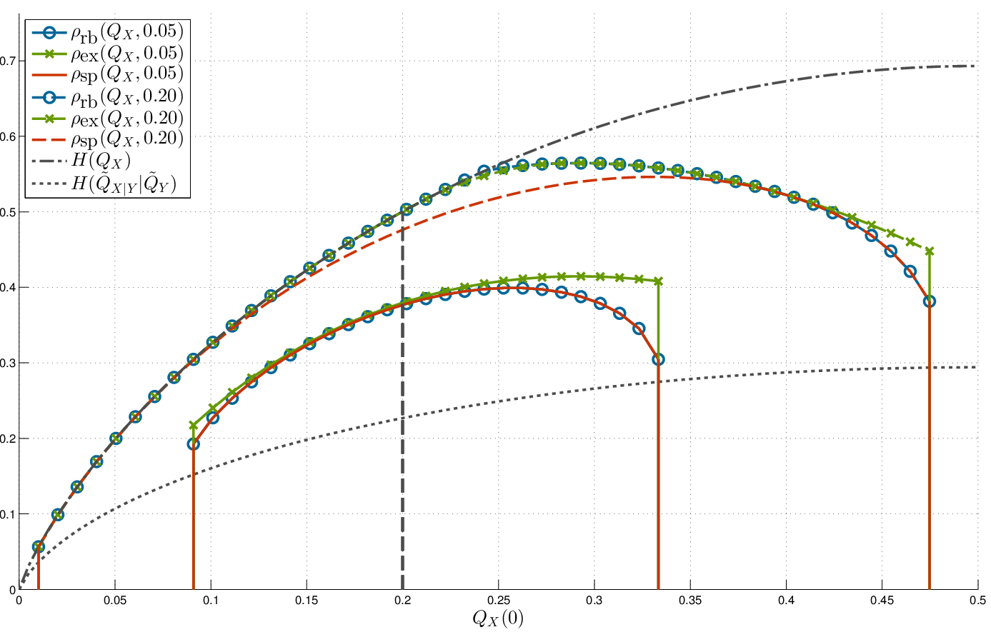
Refer to caption
Figure 1: Bounds on the optimal rate functions for the type QX​(0.25)=0.25Q_{X}(0.25)=0.25.
Refer to caption
Figure 2: Bounds on the optimal rate functions for a given 𝖤e\mathsf{E}_{e}.
Refer to caption
Figure 3: Bounds on the optimal excess-rate exponent for 𝖤e=0.05\mathsf{E}_{e}=0.05.
Refer to caption
Figure 4: Bounds on the optimal excess-rate exponent for 𝖤e=0.2\mathsf{E}_{e}=0.2.

VIII Summary

In this paper, we have considered the trade-off between error and excess-rate exponents for variable-rate SW coding. The cases of fixed-rate coding and variable-rate coding under average constraints may be considered as two extreme points in this trade-off. In fixed-rate coding the same rate is assigned to all possible types, and so, the maximal excess-rate exponent is achieved, but at the price of minimal error exponent. In average-rate coding, the main concern is the coding of the true type of the source, and all other types are sent uncoded. The resulting error exponent is maximal, but at the price of minimal excess-rate exponent. Thus, for a coding system with more stringent instantaneous rate demands, it is necessary to lose some of the gains in error exponent of variable-rate coding, and improve the excess-rate exponent. In this work, we have derived bounds on rate functions which achieve the optimal trade-off, and analyzed their excess-rate performance, for a given requirement on the error exponent.

Before we conclude, we briefly outline two possible extensions. In many practical cases, there is some uncertainty regarding the source PX​Y=PX×PY|XP_{XY}=P_{X}\times P_{Y|X}. Clearly, if independence between XX and YY is a possible scenario, then in this worst case, the side information 𝐲\mathbf{y} is useless (when no feedback link exists). In other cases, it may be known that PX​Y∈ℱ⊂𝒬⁡(𝒳×𝒴)P_{XY}\in{\cal F}\subset{\cal Q}({\cal X}\times{\cal Y}) for some family of distributions ℱ{\cal F}. In this case, a possible requirement is that the rate function ρ⁡(QX)\rho(Q_{X}) will be chosen to achieve error exponent of 𝖤e\mathsf{E}_{e} uniformly for all sources in ℱ{\cal F}. With a slight change and abuse of notation, we define, e.g. the infimum optimal rate function for the source PX​YP_{XY} as ρ¯∗​(QX,𝖤e,PX​Y)\underline{\rho}^{*}(Q_{X},\mathsf{E}_{e};P_{XY}) and the optimal rate function for the family ℱ{\cal F} as

ρ¯∗​(QX,𝖤e,ℱ)≜maxPX​Y∈ℱ⁡ρ¯∗​(QX,𝖤e,PX​Y).\underline{\rho}^{*}(Q_{X},\mathsf{E}_{e};{\cal F})\triangleq\max_{P_{XY}\in{\cal F}}\underline{\rho}^{*}(Q_{X},\mathsf{E}_{e};P_{XY}). (89)

This maximization is (relatively) easy to perform if, e.g., the conditional probability PY|XP_{Y|X} is known exactly, and in addition, a nominal P~X\tilde{P}_{X} is known such that the actual PXP_{X} satisfies D(P~X||PX)≤𝖴D(\tilde{P}_{X}||P_{X})\leq\mathsf{U}, for some given uncertainty level 𝖴>0\mathsf{U}>0 (recall Pinsker’s inequality [37, Lemma 11.6.1] and see also the discussion in [38]). A direction for future research is to derive bounds on optimal rate functions and their excess-rate performance which are robust for source uncertainty of various kinds.

In this paper, we have focused on the SW scenario in which the side information vector 𝐲\mathbf{y} is known exactly to the source. Similar techniques can also be applied to the more general case of SW coding, where the side information is also encoded. In this case, there are two encoders, sns_{n} for encoding 𝐱\mathbf{x} and sn′s_{n}^{\prime} for encoding 𝐲\mathbf{y}, while the central decoder σn\sigma_{n} now uses both codewords sn​(𝐱)s_{n}(\mathbf{x}) and sn′​(𝐲)s^{\prime}_{n}(\mathbf{y}). For type-dependent, variable-rate codes, two rate functions ρX​(QX)\rho_{X}(Q_{X}) and ρY​(QY)\rho_{Y}(Q_{Y}) may be defined accordingly. While bounds on the resulting error exponent may be derived, the trade-off in this case is more complicated. First, there are two excess-rate exponents, one for each of the decoders. Second, a trickle of coordination might be required between the two encoders in order to ensure a required error exponent.Specifically, at least one of the encoders needs to know the current rate (or equivalently, the type class of the current source block) of the other encoder.

Acknowledgments

The authors would like to thank the Associate Editor, Jun Chen, for providing them the unpublished manuscript [18], and for his useful comments. Specifically, the proof of Theorem 5 follows from the proof of Theorem 2 which is a reproduction of [18, Theorem 1]. Useful comments made by the anonymous referees are also acknowledged with thanks.

Appendix A

Proof:

Upper bound (26): Follows exactly as in the proof of [18, Theorem 1].

Lower bound (27): The proof of the achievable bound is also very similar to the proof of [18, Theorem 1], with a slight modification. For completeness, we provide a proof here.

For brevity, we will omit the notation of the dependence of R¯​(QX,𝒮)\overline{R}(Q_{X};{\cal S}) in 𝒮{\cal S} and denote it by R¯​(QX)\overline{R}(Q_{X}). Assume that QX∈int⁡𝒬⁡(𝒳),Q_{X}\in\interior{\cal Q}({\cal X}), and QX∈𝒫n0​(𝒳)Q_{X}\in{\cal P}_{n_{0}}({\cal X}) for some minimal n0∈ℕn_{0}\in\mathbb{N}. Since the statement in (27) is only about the conditional error exponent of the type QXQ_{X}, it is clear that the SW codes constructed, may only encode 𝐱∈𝒯n​(QX)\mathbf{x}\in{\cal T}_{n}(Q_{X}), and so only block lengths nmodn0≠0n\mod n_{0}\neq 0 should be considered, as otherwise 𝒯n​(QX){\cal T}_{n}(Q_{X}) is empty, and the conditional error probability is 00, by definition.

Let δ>0\delta>0 be given, and let 𝒞{\cal C} be a sequence of constant composition channel codes of type QX(n)→QXQ_{X}^{(n)}\to Q_{X}, asymptotic rate lim infn→∞log⁡|𝒞n|n≥H⁡(QX)−R¯​(QX)−δ2\liminf_{n\to\infty}\frac{\log|{\cal C}_{n}|}{n}\geq H(Q_{X})-\overline{R}(Q_{X})-\frac{\delta}{2}, which also achieves the infimum reliability function for the channel PY|XP_{Y|X}, i.e.

lim infn→∞−1nlogpe(𝒞n)≥E¯e∗(H(QX)−R¯(QX),QX,PY|X)−δ.\liminf_{n\to\infty}-\frac{1}{n}\log p_{e}({\cal C}_{n})\geq\underline{E}_{e}^{*}(H(Q_{X})-\overline{R}(Q_{X}),Q_{X},P_{Y|X})-\delta. (A.1)

From Lemma 26, it can be assumed w.l.o.g. that for nn sufficiently large, whenever, nmodn0=0n\mod n_{0}=0, the codebook satisfies 𝒞n∈𝒯n​(QX){\cal C}_{n}\in{\cal T}_{n}(Q_{X}). Now, assume that nn is sufficiently large and that nmodn0≠0n\mod n_{0}\neq 0. From the covering lemma [39, Section 6, Covering Lemma 2], one can find

Tn=exp⁡[n⁡(R¯​(QX)+δ)]T_{n}=\exp\left[n\left(\overline{R}(Q_{X})+\delta\right)\right] (A.2)

permutations {πn,t}t=1Tn\{\pi_{n,t}\}_{t=1}^{T_{n}}, such that 𝒯n​(QX)=⋃t=1Tnπn,t​(𝒞n){\cal T}_{n}(Q_{X})=\bigcup_{t=1}^{T_{n}}\pi_{n,t}({\cal C}_{n}), where πn,t​(𝒞n)\pi_{n,t}({\cal C}_{n}) means that the same permutation πn,t​(⋅)\pi_{n,t}(\cdot) operates on codewords in the codebook. Since the channel PY|XP_{Y|X} is memoryless then clearly pe​(π⁡(𝒞n))=pe​(𝒞n)p_{e}(\pi({\cal C}_{n}))=p_{e}({\cal C}_{n}) for any permutation π\pi, since the decoder can always apply the inverse permutation on 𝐲\mathbf{y} and decode as if the codebook is 𝒞n{\cal C}_{n}. Let us define the following sequence of SW codes 𝒮∗={𝒮=∗n(sn∗,σn∗)}{\cal S}^{*}=\{{\cal S}{}_{n}^{*}=(s_{n}^{*},\sigma_{n}^{*})\} from the channel codes 𝒞={𝒞n=(fn,φn)}{\cal C}=\{{\cal C}_{n}=(f_{n},\varphi_{n})\}.

  • •

    Codebook Construction: Generate the codebook 𝒞n{\cal C}_{n} and enumerate the permutations {πn,t}t=1Tn\{\pi_{n,t}\}_{t=1}^{T_{n}} such that 𝒯n​(QX)=⋃l=1Tnπn,t​(𝒞n){\cal T}_{n}(Q_{X})=\bigcup_{l=1}^{T_{n}}\pi_{n,t}({\cal C}_{n}). The above information is revealed to both the encoder and the decoder off-line.

  • •

    Encoding: Upon observing 𝐱\mathbf{x}, determine its empirical distribution Q^𝐱\hat{Q}_{\mathbf{x}}. If Q^𝐱≠QX\hat{Q}_{\mathbf{x}}\not=Q_{X} the codeword is sn∗​(𝐱)=0s_{n}^{*}(\mathbf{x})=0. Else, find t∗​(𝐱)≜min⁡{t′:𝐱∈πn,t′​(𝒞n​(QX))}t^{*}(\mathbf{x})\triangleq\min\{t^{\prime}:\mathbf{x}\in\pi_{n,t^{\prime}}({\cal C}_{n}(Q_{X}))\}. The codeword is sn∗​(𝐱)=(1,τ⁡(t∗​(𝐱)))s_{n}^{*}(\mathbf{x})=(1,\tau(t^{*}(\mathbf{x}))) where τ⁡(t)\tau(t) is the binary representation of tt in ⌈log2⁡Tn⌉\left\lceil\log_{2}T_{n}\right\rceil bits.

  • •

    Decoding: If s(𝐱)∗n=0s{}_{n}^{*}(\mathbf{x})=0 then declare an error. Else, recover from sn∗​(𝐱)s_{n}^{*}(\mathbf{x}) the permutation π=πn,t⁡(𝐱)\pi=\pi_{n,t(\mathbf{x})}. Find t^​(𝐲)≜t∗​(π⁡(φn​(π−1​(𝐲)))CLOSE\hat{t}(\mathbf{y})\triangleq t^{*}(\pi(\varphi_{n}(\pi^{-1}(\mathbf{y}))), and if t^​(𝐲)=t∗​(𝐱)\hat{t}(\mathbf{y})=t^{*}(\mathbf{x}) then decode 𝐱^=π⁡(φn​(π−1​(𝐲)))\hat{\mathbf{x}}=\pi(\varphi_{n}(\pi^{-1}(\mathbf{y}))), and otherwise declare an error.

The conditional average rate of 𝒮∗{\cal S}^{*} satisfies lim supn→∞𝔼⁡[r∗​(𝐗)|𝐗∈𝒯n​(QX)]=R¯​(QX)+δ\limsup_{n\to\infty}\mathbb{E}[r^{*}(\mathbf{X})|\mathbf{X}\in{\cal T}_{n}(Q_{X})]=\overline{R}(Q_{X})+\delta. Since all source blocks in 𝒯n​(QX){\cal T}_{n}(Q_{X}) are equiprobable, the conditional error probability satisfies

lim infn→∞−1nlogℙ(σ(s(𝐗)∗n,𝐘)∗n≠𝐗|𝐗∈𝒯n(QX))\displaystyle\liminf_{n\to\infty}-\frac{1}{n}\log\mathbb{P}(\sigma{}_{n}^{*}(s{}_{n}^{*}(\mathbf{X}),\mathbf{Y})\neq\mathbf{X}|\mathbf{X}\in{\cal T}_{n}(Q_{X})) ≥lim infn→∞−1nlogℙ(φ(𝐘)n≠𝐗|𝐗∈𝒯n(QX))\displaystyle\geq\liminf_{n\to\infty}-\frac{1}{n}\log\mathbb{P}(\varphi{}_{n}(\mathbf{Y})\neq\mathbf{X}|\mathbf{X}\in{\cal T}_{n}(Q_{X}))
=E¯e∗​(H⁡(QX)−R¯​(QX),QX,PY|X)−δ,\displaystyle=\underline{E}_{e}^{*}(H(Q_{X})-\overline{R}(Q_{X}),Q_{X},P_{Y|X})-\delta, (A.3)

where it should be emphasized that whenever nmodn0≠0n\mod n_{0}\neq 0 then ℙ(σ(s(𝐗)∗n,𝐘)∗n≠𝐗|𝐗∈𝒯n(QX))=0\mathbb{P}(\sigma{}_{n}^{*}(s{}_{n}^{*}(\mathbf{X}),\mathbf{Y})\neq\mathbf{X}|\mathbf{X}\in{\cal T}_{n}(Q_{X}))=0 by convention. The result follows since δ>0\delta>0 was arbitrary. Before concluding the proof, we make the following remark.

Remark 19.

In the proof, the actual choice of the decoder was implicit since the SW codes are constructed from channel codes. However, as is well known, the optimal decoder in terms of minimum error probability is to decode 𝐱~∈𝒯n​(QX)∩sn−1​(sn​(𝐱))\tilde{\mathbf{x}}\in{\cal T}_{n}(Q_{X})\cap s_{n}^{-1}(s_{n}(\mathbf{x})) that maximizes P𝐗|𝐘​(𝐱~|𝐲)P_{\mathbf{X}|\mathbf{Y}}(\tilde{\mathbf{x}}|\mathbf{y}). Since all 𝐱~∈sn−1​(sn​(𝐱))\tilde{\mathbf{x}}\in s_{n}^{-1}(s_{n}(\mathbf{x})) are in the type class QXQ_{X}, they have the same probability P𝐗​(𝐱~)P_{\mathbf{X}}(\tilde{\mathbf{x}}), so this decoding rule is equivalent to maximizing P𝐘|𝐗​(𝐲|𝐱~)P_{\mathbf{Y}|\mathbf{X}}(\mathbf{y}|\tilde{\mathbf{x}}), which is a maximum likelihood (ML) decoding rule. Nonetheless, there are cases in which other decoders, such as the minimum conditional entropy decoder, also achieve the same error exponent (see Appendix C for a precise definition). This decoder has the merit of not depending on PX​YP_{XY} and is therefore a universal decoder.

∎

Proof:

Since |𝒫n​(𝒳)|≤(n+1)|𝒳||{\cal P}_{n}({\cal X})|\leq(n+1)^{|{\cal X}|}, the error probability satisfies

pe​(𝒮n)\displaystyle p_{e}({\cal S}_{n}) =∑QX∈𝒫n​(𝒳)ℙ⁡(𝒯n​(QX))​ℙ​(𝐗^≠𝐗|𝐗∈𝒯n​(QX))\displaystyle=\sum_{Q_{X}\in{\cal P}_{n}({\cal X})}\mathbb{P}({\cal T}_{n}(Q_{X}))\mathbb{P}(\hat{\mathbf{X}}\neq\mathbf{X}|\mathbf{X}\in{\cal T}_{n}(Q_{X})) (A.4)
≐maxQX∈𝒫n​(𝒳)e−nD(QX||PX)⋅ℙ(𝐗^≠𝐗|𝐗∈𝒯n(QX))\displaystyle\doteq\max_{Q_{X}\in{\cal P}_{n}({\cal X})}e^{-nD\left(Q_{X}||P_{X}\right)}\cdot\mathbb{P}(\hat{\mathbf{X}}\neq\mathbf{X}|\mathbf{X}\in{\cal T}_{n}(Q_{X})) (A.5)
=exp(−n⋅minQX∈𝒫n​(𝒳){D(QX||PX)−1nlogℙ(𝐗^≠𝐗|𝐗∈𝒯n(QX))}).\displaystyle=\exp\left(-n\cdot\min_{Q_{X}\in{\cal P}_{n}({\cal X})}\left\{D\left(Q_{X}||P_{X}\right)-\frac{1}{n}\log\mathbb{P}(\hat{\mathbf{X}}\neq\mathbf{X}|\mathbf{X}\in{\cal T}_{n}(Q_{X}))\right\}\right). (A.6)

Now, for every ϵ>0\epsilon>0, let QX∗∈𝒫⁡(𝒳)Q_{X}^{*}\in{\cal P}({\cal X}) be such that

D(QX∗||PX)+lim supn→∞{−1nlogℙ(𝐗^≠𝐗|𝐗∈𝒯n(QX∗))}≤infQX∈𝒫⁡(𝒳){D(QX||PX)+lim supn→∞{−1nlogℙ(𝐗^≠𝐗|𝐗∈𝒯n(QX))}}+ϵD\left(Q_{X}^{*}||P_{X}\right)+\limsup_{n\to\infty}\left\{-\frac{1}{n}\log\mathbb{P}(\hat{\mathbf{X}}\neq\mathbf{X}|\mathbf{X}\in{\cal T}_{n}(Q_{X}^{*}))\right\}\leq\\ \inf_{Q_{X}\in{\cal P}({\cal X})}\left\{D\left(Q_{X}||P_{X}\right)+\limsup_{n\to\infty}\left\{-\frac{1}{n}\log\mathbb{P}(\hat{\mathbf{X}}\neq\mathbf{X}|\mathbf{X}\in{\cal T}_{n}(Q_{X}))\right\}\right\}+\epsilon (A.7)

and let m0m_{0} be sufficiently large so that

supn>m0{−1n​log⁡ℙ⁡(𝐗^≠𝐗|𝐗∈𝒯n​(QX∗))}≤lim supn→∞{−1n​log⁡ℙ⁡(𝐗^≠𝐗|𝐗∈𝒯n​(QX∗))}+ϵ.\sup_{n>m_{0}}\left\{-\frac{1}{n}\log\mathbb{P}(\hat{\mathbf{X}}\neq\mathbf{X}|\mathbf{X}\in{\cal T}_{n}(Q_{X}^{*}))\right\}\leq\limsup_{n\to\infty}\left\{-\frac{1}{n}\log\mathbb{P}(\hat{\mathbf{X}}\neq\mathbf{X}|\mathbf{X}\in{\cal T}_{n}(Q_{X}^{*}))\right\}+\epsilon. (A.8)

Then,

ℰe+​(𝒮)\displaystyle{\cal E}_{e}^{+}({\cal S}) =lim supn→∞minQX∈𝒫n​(𝒳){D(QX||PX)−1nlogℙ(𝐗^≠𝐗|𝐗∈𝒯n(QX))}\displaystyle=\limsup_{n\to\infty}\min_{Q_{X}\in{\cal P}_{n}({\cal X})}\left\{D\left(Q_{X}||P_{X}\right)-\frac{1}{n}\log\mathbb{P}(\hat{\mathbf{X}}\neq\mathbf{X}|\mathbf{X}\in{\cal T}_{n}(Q_{X}))\right\} (A.9)
=limm→∞supn≥mminQX∈𝒫n​(𝒳){D(QX||PX)−1nlogℙ(𝐗^≠𝐗|𝐗∈𝒯n(QX))}\displaystyle=\lim_{m\to\infty}\sup_{n\geq m}\min_{Q_{X}\in{\cal P}_{n}({\cal X})}\left\{D\left(Q_{X}||P_{X}\right)-\frac{1}{n}\log\mathbb{P}(\hat{\mathbf{X}}\neq\mathbf{X}|\mathbf{X}\in{\cal T}_{n}(Q_{X}))\right\} (A.10)
=(a)limm→∞supn≥minfQX∈𝒫⁡(𝒳){D(QX||PX)−1nlogℙ(𝐗^≠𝐗|𝐗∈𝒯n(QX))}\displaystyle\overset{{\scriptstyle(a)}}{=}\lim_{m\to\infty}\sup_{n\geq m}\inf_{Q_{X}\in{\cal P}({\cal X})}\left\{D\left(Q_{X}||P_{X}\right)-\frac{1}{n}\log\mathbb{P}(\hat{\mathbf{X}}\neq\mathbf{X}|\mathbf{X}\in{\cal T}_{n}(Q_{X}))\right\} (A.11)
≤supn≥m0infQX∈𝒫⁡(𝒳){D(QX||PX)−1nlogℙ(𝐗^≠𝐗|𝐗∈𝒯n(QX))}\displaystyle\leq\sup_{n\geq m_{0}}\inf_{Q_{X}\in{\cal P}({\cal X})}\left\{D\left(Q_{X}||P_{X}\right)-\frac{1}{n}\log\mathbb{P}(\hat{\mathbf{X}}\neq\mathbf{X}|\mathbf{X}\in{\cal T}_{n}(Q_{X}))\right\} (A.12)
≤infQX∈𝒫⁡(𝒳){D(QX||PX)+supn≥m0{−1nlogℙ(𝐗^≠𝐗|𝐗∈𝒯n(QX))}}\displaystyle\leq\inf_{Q_{X}\in{\cal P}({\cal X})}\left\{D\left(Q_{X}||P_{X}\right)+\sup_{n\geq m_{0}}\left\{-\frac{1}{n}\log\mathbb{P}(\hat{\mathbf{X}}\neq\mathbf{X}|\mathbf{X}\in{\cal T}_{n}(Q_{X}))\right\}\right\} (A.13)
≤D(QX∗||PX)+supn>m0{−1nlogℙ(𝐗^≠𝐗|𝐗∈𝒯n(QX∗))}\displaystyle\leq D\left(Q_{X}^{*}||P_{X}\right)+\sup_{n>m_{0}}\left\{-\frac{1}{n}\log\mathbb{P}(\hat{\mathbf{X}}\neq\mathbf{X}|\mathbf{X}\in{\cal T}_{n}(Q_{X}^{*}))\right\} (A.14)
≤(b)infQX∈𝒫⁡(𝒳){D(QX||PX)+lim supn→∞{−1nlogℙ(𝐗^≠𝐗|𝐗∈𝒯n(QX))}}+2ϵ\displaystyle\overset{{\scriptstyle(b)}}{\leq}\inf_{Q_{X}\in{\cal P}({\cal X})}\left\{D\left(Q_{X}||P_{X}\right)+\limsup_{n\to\infty}\left\{-\frac{1}{n}\log\mathbb{P}(\hat{\mathbf{X}}\neq\mathbf{X}|\mathbf{X}\in{\cal T}_{n}(Q_{X}))\right\}\right\}+2\epsilon (A.15)
≤(c)infQX∈𝒫⁡(𝒳){D(QX||PX)+E¯e∗(H(QX)−R¯(QX;𝒮),QX,PY|X)}+2ϵ\displaystyle\overset{{\scriptstyle(c)}}{\leq}\inf_{Q_{X}\in{\cal P}({\cal X})}\left\{D\left(Q_{X}||P_{X}\right)+\overline{E}_{e}^{*}(H(Q_{X})-\overline{R}(Q_{X};{\cal S}),Q_{X},P_{Y|X})\right\}+2\epsilon (A.16)

where (a)(a) is because, by assumption, if 𝒯n​(QX){\cal T}_{n}(Q_{X}) is empty then ℙ⁡(𝐗^≠𝐗|𝐗∈𝒯n​(QX))=0\mathbb{P}(\hat{\mathbf{X}}\neq\mathbf{X}|\mathbf{X}\in{\cal T}_{n}(Q_{X}))=0 , and (b)(b) is from (A.7) and (A.8). The inequality (c)(c) is due to the upper bound of Theorem 2. ∎

Proof:

The excess-rate exponent at the target rate 𝖱\mathsf{R} is

pr​(𝒮n,𝖱)\displaystyle p_{r}({\cal S}_{n},\mathsf{R}) =∑QX∈𝒫n​(𝒳)ℙ⁡(𝒯n​(QX))​ℙ​(r⁡(𝐗)≥𝖱|𝐗∈𝒯n​(QX))\displaystyle=\sum_{Q_{X}\in{\cal P}_{n}({\cal X})}\mathbb{P}({\cal T}_{n}(Q_{X}))\mathbb{P}(r(\mathbf{X})\geq\mathsf{R}|\mathbf{X}\in{\cal T}_{n}(Q_{X})) (A.17)
≐exp(−n⋅minQX∈𝒫n​(𝒳){D(QX||PX)−1nlogℙ(r(𝐗)≥𝖱|𝐗∈𝒯n(QX))}).\displaystyle\doteq\exp\left(-n\cdot\min_{Q_{X}\in{\cal P}_{n}({\cal X})}\left\{D(Q_{X}||P_{X})-\frac{1}{n}\log\mathbb{P}(r(\mathbf{X})\geq\mathsf{R}|\mathbf{X}\in{\cal T}_{n}(Q_{X}))\right\}\right). (A.18)

Now, let ϵ>0\epsilon>0 be given and let m0m_{0} be sufficiently large such that

lim infn→∞{D(QX||PX)−1nlogℙ(r(𝐗)≥𝖱|𝐗∈𝒯n(QX))}≤infn≥m0minQX∈𝒫n​(𝒳){D(QX||PX)+lim infn→∞{−1nlogℙ(r(𝐗)≥𝖱|𝐗∈𝒯n(QX))}}+ϵ.\liminf_{n\to\infty}\left\{D(Q_{X}||P_{X})-\frac{1}{n}\log\mathbb{P}(r(\mathbf{X})\geq\mathsf{R}|\mathbf{X}\in{\cal T}_{n}(Q_{X}))\right\}\\ \leq\inf_{n\geq m_{0}}\min_{Q_{X}\in{\cal P}_{n}({\cal X})}\left\{D(Q_{X}||P_{X})+\liminf_{n\to\infty}\left\{-\frac{1}{n}\log\mathbb{P}(r(\mathbf{X})\geq\mathsf{R}|\mathbf{X}\in{\cal T}_{n}(Q_{X}))\right\}\right\}+\epsilon. (A.19)

Also, choose QX∗∈𝒫n0​(𝒳)Q_{X}^{*}\in{\cal P}_{n_{0}}({\cal X}) such that

D(QX∗||PX)+lim infn→∞{−1nlogℙ(r(𝐗)≥𝖱|𝐗∈𝒯n(QX∗))}≤infQX∈𝒫⁡(𝒳){D(QX||PX)+lim infn→∞{−1nlogℙ(r(𝐗)≥𝖱|𝐗∈𝒯n(QX))}}+ϵ.D(Q_{X}^{*}||P_{X})+\liminf_{n\to\infty}\left\{-\frac{1}{n}\log\mathbb{P}(r(\mathbf{X})\geq\mathsf{R}|\mathbf{X}\in{\cal T}_{n}(Q_{X}^{*}))\right\}\\ \leq\inf_{Q_{X}\in{\cal P}({\cal X})}\left\{D(Q_{X}||P_{X})+\liminf_{n\to\infty}\left\{-\frac{1}{n}\log\mathbb{P}(r(\mathbf{X})\geq\mathsf{R}|\mathbf{X}\in{\cal T}_{n}(Q_{X}))\right\}\right\}+\epsilon. (A.20)

Then,

ℰr​(𝒮,𝖱)\displaystyle{\cal E}_{r}({\cal S},\mathsf{R}) =lim infn→∞minQX∈𝒫n​(𝒳){D(QX||PX)−1nlogℙ(r(𝐗)≥𝖱|𝐗∈𝒯n(QX))}\displaystyle=\liminf_{n\to\infty}\min_{Q_{X}\in{\cal P}_{n}({\cal X})}\left\{D(Q_{X}||P_{X})-\frac{1}{n}\log\mathbb{P}(r(\mathbf{X})\geq\mathsf{R}|\mathbf{X}\in{\cal T}_{n}(Q_{X}))\right\} (A.21)
≤(a)infn≥m0minQX∈𝒫n​(𝒳){D(QX||PX)−1nlogℙ(r(𝐗)≥𝖱|𝐗∈𝒯n(QX))}+ϵ\displaystyle\overset{{\scriptstyle(a)}}{\leq}\inf_{n\geq m_{0}}\min_{Q_{X}\in{\cal P}_{n}({\cal X})}\left\{D(Q_{X}||P_{X})-\frac{1}{n}\log\mathbb{P}(r(\mathbf{X})\geq\mathsf{R}|\mathbf{X}\in{\cal T}_{n}(Q_{X}))\right\}+\epsilon (A.22)
≤(b)infn≥m0{D(QX∗||PX)−1nlogℙ(r(𝐗)≥𝖱|𝐗∈𝒯n(QX∗))}+ϵ\displaystyle\overset{{\scriptstyle(b)}}{\leq}\inf_{n\geq m_{0}}\left\{D(Q_{X}^{*}||P_{X})-\frac{1}{n}\log\mathbb{P}(r(\mathbf{X})\geq\mathsf{R}|\mathbf{X}\in{\cal T}_{n}(Q_{X}^{*}))\right\}+\epsilon (A.23)
=D(QX∗||PX)+infn≥m0{−1nlogℙ(r(𝐗)≥𝖱|𝐗∈𝒯n(QX∗))}+ϵ\displaystyle=D(Q_{X}^{*}||P_{X})+\inf_{n\geq m_{0}}\left\{-\frac{1}{n}\log\mathbb{P}(r(\mathbf{X})\geq\mathsf{R}|\mathbf{X}\in{\cal T}_{n}(Q_{X}^{*}))\right\}+\epsilon (A.24)
≤{D(QX∗||PX)+limm→∞infn≥m−1nlogℙ(r(𝐗)≥𝖱|𝐗∈𝒯n(QX∗))}+ϵ\displaystyle\leq\left\{D(Q_{X}^{*}||P_{X})+\lim_{m\to\infty}\inf_{n\geq m}-\frac{1}{n}\log\mathbb{P}(r(\mathbf{X})\geq\mathsf{R}|\mathbf{X}\in{\cal T}_{n}(Q_{X}^{*}))\right\}+\epsilon (A.25)
≤(c)infQX∈𝒫⁡(𝒳){D(QX||PX)+lim infn→∞{−1nlogℙ(r(𝐗)≥𝖱|𝐗∈𝒯n(QX))}}+2ϵ\displaystyle\overset{{\scriptstyle(c)}}{\leq}\inf_{Q_{X}\in{\cal P}({\cal X})}\left\{D(Q_{X}||P_{X})+\liminf_{n\to\infty}\left\{-\frac{1}{n}\log\mathbb{P}(r(\mathbf{X})\geq\mathsf{R}|\mathbf{X}\in{\cal T}_{n}(Q_{X}))\right\}\right\}+2\epsilon

where (a)(a) is due to (A.19), (b)(b) is because there exists l∈ℕl\in\mathbb{N} so that l⋅n0>m0l\cdot n_{0}>m_{0} and then QX∗∈𝒫n0​(𝒳)⊂𝒫l⋅n0​(𝒳)Q_{X}^{*}\in{\cal P}_{n_{0}}({\cal X})\subset{\cal P}_{l\cdot n_{0}}({\cal X}), and (c)(c) is due to (A.20). As ϵ>0\epsilon>0 is arbitrary we get the desired result. ∎

Proof:

We will use the following two lemmas:

Lemma 20.

Let QX,QX′∈𝒫n​(𝒳)Q_{X},Q^{\prime}_{X}\in{\cal P}_{n}({\cal X}) and assume that1010 10 For two different types in 𝒫n​(𝒳){\cal P}_{n}({\cal X}), the minimal variation distance is 2n\frac{2}{n}. ‖QX−QX′‖=2​d∗n||Q_{X}-Q^{\prime}_{X}||=\frac{2d^{*}}{n} where d∗>0d^{*}>0. If 𝐱∈𝒯n​(QX)\mathbf{x}\in{\cal T}_{n}(Q_{X}) then

min𝐳∈𝒯n​(QX′)⁡dH​(𝐱,𝐳)≤d∗.\min_{\mathbf{z}\in{\cal T}_{n}(Q^{\prime}_{X})}d_{\textnormal{\scriptsize H}}(\mathbf{x},\mathbf{z})\leq d^{*}. (A.26)
Proof:

We prove this Lemma by modifying the vector 𝐱∈𝒯n​(QX)\mathbf{x}\in{\cal T}_{n}(Q_{X}) into a vector 𝐱′∈𝒯n​(QX′)\mathbf{x}^{\prime}\in{\cal T}_{n}(Q^{\prime}_{X}) by less than d∗d^{*} letter substitutions. Clearly, for some letters x1−,x1+∈𝒳x_{1}^{-},x_{1}^{+}\in{\cal X} we have QX​(x1−)<QX′​(x1−)Q_{X}(x_{1}^{-})<Q^{\prime}_{X}(x_{1}^{-}) and QX​(x1+)>QX′​(x1+)Q_{X}(x_{1}^{+})>Q^{\prime}_{X}(x_{1}^{+}). Find an index i1i_{1} such that the iith entry of 𝐱\mathbf{x} is x1+x_{1}^{+} and change it to x1−x_{1}^{-}. Denote the resulting vector by 𝐱1\mathbf{x}_{1}, and let its type by QX(1)Q_{X}^{(1)}. If, QX(1)=QX′Q_{X}^{(1)}=Q^{\prime}_{X} then we have found a vector 𝐱′∈𝒯n​(QX′)\mathbf{x}^{\prime}\in{\cal T}_{n}(Q^{\prime}_{X}) such that dH​(𝐱,𝐱′)≤1≤d∗d_{\textnormal{\scriptsize H}}(\mathbf{x},\mathbf{x}^{\prime})\leq 1\leq d^{*} and thus we are done. Otherwise, we have

‖QX′−QX(1)‖=2​(d∗−1)n.||Q^{\prime}_{X}-Q_{X}^{(1)}||=\frac{2(d^{*}-1)}{n}. (A.27)

In this case, repeat the same steps for 𝐱1\mathbf{x}_{1}, and at each step, the variation distance between QX′Q^{\prime}_{X} and QX(k)Q_{X}^{(k)} decreases by 2n\frac{2}{n}. Thus, after at most d∗d^{*} stages, a vector 𝐱(d∗)∈𝒯n​(QX′)\mathbf{x}^{(d^{*})}\in{\cal T}_{n}(Q^{\prime}_{X}) is found, such that dH​(𝐱,𝐱′)≤d∗d_{\textnormal{\scriptsize H}}(\mathbf{x},\mathbf{x}^{\prime})\leq d^{*}.∎

Lemma 21.

Let QX∈𝒫n​(𝒳)Q_{X}\in{\cal P}_{n}({\cal X}) and 𝐱∈𝒯n​(QX)\mathbf{x}\in{\cal T}_{n}(Q_{X}). For 1≤k<n1\leq k<n we have

||Q^𝐱−Q^𝐱⁡(1:n−k)||<|𝒳|⋅kn−k.||\hat{Q}_{\mathbf{x}}-\hat{Q}_{\mathbf{x}(1:n-k)}||<|{\cal X}|\cdot\frac{k}{n-k}. (A.28)
Proof:

For any given letter x∈𝒳x\in{\cal X}, we denote Q^𝐱​(x)=mn\hat{Q}_{\mathbf{x}}(x)=\frac{m}{n}, and analyze

|Q^𝐱(x)−Q^𝐱⁡(1:n−k)(x)|.|\hat{Q}_{\mathbf{x}}(x)-\hat{Q}_{\mathbf{x}(1:n-k)}(x)|. (A.29)

The largest difference possible is either when 𝐱⁡(i)=x\mathbf{x}(i)=x for min⁡{k,m}\min\{k,m\} letters out of n−k+1≤i≤nn-k+1\leq i\leq n or 𝐱⁡(i)≠x\mathbf{x}(i)\neq x for all n−k+1≤i≤nn-k+1\leq i\leq n. In the former case, when m≥km\geq k, then

|Q^𝐱(x)−Q^𝐱⁡(1:n−k)(x)|\displaystyle|\hat{Q}_{\mathbf{x}}(x)-\hat{Q}_{\mathbf{x}(1:n-k)}(x)| =|mn−m−kn−k|=mn−m−kn−k\displaystyle=\left|\frac{m}{n}-\frac{m-k}{n-k}\right|=\frac{m}{n}-\frac{m-k}{n-k} (A.30)
<mn−m−kn<kn−k\displaystyle<\frac{m}{n}-\frac{m-k}{n}<\frac{k}{n-k} (A.31)

and when m<km<k then

|Q^𝐱(x)−Q^𝐱⁡(1:n−k)(x)|\displaystyle|\hat{Q}_{\mathbf{x}}(x)-\hat{Q}_{\mathbf{x}(1:n-k)}(x)| =|mn−0n−k|=mn\displaystyle=\left|\frac{m}{n}-\frac{0}{n-k}\right|=\frac{m}{n} (A.32)
<kn<kn−k.\displaystyle<\frac{k}{n}<\frac{k}{n-k}. (A.33)

In the later case

|Q^𝐱(x)−Q^𝐱⁡(1:n−k)(x)|\displaystyle|\hat{Q}_{\mathbf{x}}(x)-\hat{Q}_{\mathbf{x}(1:n-k)}(x)| =|mn−mn−k|=mn−k−mn\displaystyle=\left|\frac{m}{n}-\frac{m}{n-k}\right|=\frac{m}{n-k}-\frac{m}{n} (A.34)
≤mn−k−m−kn−k=kn−k.\displaystyle\leq\frac{m}{n-k}-\frac{m-k}{n-k}=\frac{k}{n-k}. (A.35)

The result follows by summing over x∈𝒳x\in{\cal X}. ∎ We can now prove Theorem 5. Let ϵ>0\epsilon>0 be given, and find n0n_{0} sufficiently large such that for any QX′∈𝒫⁡(𝒳)Q^{\prime}_{X}\in{\cal P}({\cal X}) there exists QX∈𝒫n0​(𝒳)∩int⁡𝒬⁡(𝒳)Q_{X}\in{\cal P}_{n_{0}}({\cal X})\cap\interior{\cal Q}({\cal X}) such that ‖QX−QX′‖≤ϵ2||Q_{X}-Q^{\prime}_{X}||\leq\frac{\epsilon}{2}. For a given pair of vectors 𝐱,𝐱′∈𝒳n\mathbf{x},\mathbf{x}^{\prime}\in{\cal X}^{n}, define the binary vector Δ𝐱𝐱′∈{0,1}n\Delta_{\mathbf{x}\mathbf{x}^{\prime}}\in\{0,1\}^{n} where

Δ𝐱𝐱′​(i)={1,𝐱​(i)≠𝐱′​(i)0,𝐱​(i)=𝐱′​(i)\Delta_{\mathbf{x}\mathbf{x}^{\prime}}(i)=\begin{cases}1,&\mathbf{x}(i)\neq\mathbf{x}^{\prime}(i)\\ 0,&\mathbf{x}(i)=\mathbf{x}^{\prime}(i)\end{cases} (A.36)

and also define ℋ𝐱𝐱′={i:𝐱⁡(i)≠𝐱′​(i)}{\cal H}_{\mathbf{x}\mathbf{x}^{\prime}}=\{i:\mathbf{x}(i)\neq\mathbf{x}^{\prime}(i)\}. Also let n1=n0​ϵ+2​n0​|𝒳|n_{1}=n_{0}\epsilon+2n_{0}|{\cal X}|. We construct the following SW codes 𝒮{\cal S} for all n>max⁡{n0,n1}n>\max\{n_{0},n_{1}\}:

  • •

    Codebook Construction:

    • –

      Compute k∗​(n)≜⌊nn0⌋k^{*}(n)\triangleq\left\lfloor\frac{n}{n_{0}}\right\rfloor.

    • –

      Assign a binary string τ1​(QX)\tau_{1}(Q_{X}) for each type in QX∈𝒫n​(𝒳)Q_{X}\in{\cal P}_{n}({\cal X}).

    • –

      Assign a binary string τ2​(a)\tau_{2}(a) for each letter x∈𝒳x\in{\cal X}. For any vector 𝐱∈𝒳m\mathbf{x}\in{\cal X}^{m}, define

      τ2​(𝐱)≜(τ2​(𝐱⁡(1)),…,τ2​(𝐱⁡(m))).\tau_{2}(\mathbf{x})\triangleq(\tau_{2}(\mathbf{x}(1)),\ldots,\tau_{2}(\mathbf{x}(m))). (A.37)
    • –

      Assign a binary string τ3​(𝐛)\tau_{3}(\mathbf{b}) for each binary vector 𝐛∈{0,1}n\mathbf{b}\in\{0,1\}^{n} such that dH​(𝟎,𝐛)≤⌈n​ϵ2⌉d_{\textnormal{\scriptsize H}}(\mathbf{0},\mathbf{b})\leq\lceil\frac{n\epsilon}{2}\rceil, where 𝟎\mathbf{0} is the all-zero vector of length nn.

    • –

      Construct the SW codes 𝒮k∗​(n)⋅n0∗​(QX)=(sk∗​(n)⋅n0,QX∗,σk∗​(n)⋅n0,QX∗){\cal S}_{k^{*}(n)\cdot n_{0}}^{*}(Q_{X})=(s_{k^{*}(n)\cdot n_{0},Q_{X}}^{*},\sigma_{k^{*}(n)\cdot n_{0},Q_{X}}^{*}) of rate ρ⁡(QX)\rho(Q_{X}) as in Theorem 2, for all Q∈X𝒫n0(𝒳)∩int𝒬(𝒳)Q{}_{X}\in{\cal P}_{n_{0}}({\cal X})\cap\interior{\cal Q}({\cal X}).

    • –

      For any given QX∈𝒫n​(𝒳)Q_{X}\in{\cal P}_{n}({\cal X}) find

      Φϵ​(QX)≜arg​minQX′∈𝒫n0​(𝒳)∩int⁡𝒬⁡(𝒳)⁡‖QX−QX′‖.\Phi_{\epsilon}(Q_{X})\triangleq\argmin_{Q^{\prime}_{X}\in{\cal P}_{n_{0}}({\cal X})\cap\interior{\cal Q}({\cal X})}||Q_{X}-Q^{\prime}_{X}||. (A.38)

    The above information is revealed to both the encoder and the decoder off-line.

  • •

    Encoding: Upon observing 𝐱\mathbf{x}, determine its empirical distribution Q^𝐱\hat{Q}_{\mathbf{x}} and find

    𝐰=arg​min𝐰¯∈𝒯k∗​(n)⋅n0​(Φϵ​(Q^𝐱))⁡dH​(𝐱⁡(1:k∗​(n)⋅n0),𝐰¯).\mathbf{w}=\argmin_{\overline{\mathbf{w}}\in{\cal T}_{k^{*}(n)\cdot n_{0}}(\Phi_{\epsilon}(\hat{Q}_{\mathbf{x}}))}d_{\textnormal{\scriptsize H}}(\mathbf{x}(1:k^{*}(n)\cdot n_{0}),\overline{\mathbf{w}}). (A.39)

    Let 𝐱′=𝐱⁡(1:k∗​(n)⋅n0)\mathbf{x}^{\prime}=\mathbf{x}(1:k^{*}(n)\cdot n_{0}), and encode the source block 𝐱\mathbf{x} as:

    sn​(𝐱)=(τ1​(Q^𝐱),τ2​(𝐰⁡(ℋ𝐱′​𝐰),τ2​(𝐱⁡(ℋ𝐱′​𝐰)),τ3​(Δ𝐱′​𝐰),τ2​(𝐱⁡(k∗​(n)⋅n0+1:n)),sk∗​(n)⋅n0,QX∗​(𝐰))CLOSE.s_{n}(\mathbf{x})=(\tau_{1}(\hat{Q}_{\mathbf{x}}),\tau_{2}(\mathbf{w}({\cal H}_{\mathbf{x}^{\prime}\mathbf{w}}),\tau_{2}(\mathbf{\mathbf{x}}({\cal H}_{\mathbf{x}^{\prime}\mathbf{w}})),\tau_{3}(\Delta_{\mathbf{x}^{\prime}\mathbf{w}}),\tau_{2}(\mathbf{x}(k^{*}(n)\cdot n_{0}+1:n)),s_{k^{*}(n)\cdot n_{0},Q_{X}}^{*}(\mathbf{w})). (A.40)
  • •

    Decoding: Upon observing 𝐲\mathbf{y} and sn​(𝐱)s_{n}(\mathbf{x}):

    • –

      From sn​(𝐱)s_{n}(\mathbf{x}), recover Q^𝐱\hat{Q}_{\mathbf{x}} and determine Φϵ​(Q^𝐱)\Phi_{\epsilon}(\hat{Q}_{\mathbf{x}}). Recover Δ𝐱′​𝐰\Delta_{\mathbf{x}^{\prime}\mathbf{w}}, 𝐰⁡(ℋ𝐱′​𝐰)\mathbf{w}({\cal H}_{\mathbf{x}^{\prime}\mathbf{w}}),𝐱⁡(ℋ𝐱′​𝐰)\mathbf{x}({\cal H}_{\mathbf{x}^{\prime}\mathbf{w}}), and 𝐱⁡(k∗​(n)⋅n0+1:n)\mathbf{x}(k^{*}(n)\cdot n_{0}+1:n).

    • –

      Generate a vector 𝐲′∈𝒴k∗​(n)⋅n0\mathbf{y}^{\prime}\in{\cal Y}^{k^{*}(n)\cdot n_{0}} as follows: For any index 1≤i≤k∗​(n)⋅n01\leq i\leq k^{*}(n)\cdot n_{0}. If Δ𝐱′​𝐰​(i)=0\Delta_{\mathbf{x}^{\prime}\mathbf{w}}(i)=0 then set 𝐲′​(i)=𝐲​(i)\mathbf{y}^{\prime}(i)=\mathbf{y}(i). Otherwise, draw 𝐲′​(i)\mathbf{y}^{\prime}(i) according to the conditional distribution PY|X(⋅|𝐰(i))P_{Y|X}(\cdot|\mathbf{w}(i)).

    • –

      Decode

      𝐰^=σk∗​(n)⋅n0,Φϵ​(Q^𝐱)∗​(sk∗​(n)⋅n0,Φϵ​(Q^𝐱)∗​(𝐰),𝐲′).\hat{\mathbf{w}}=\sigma_{k^{*}(n)\cdot n_{0},\Phi_{\epsilon}(\hat{Q}_{\mathbf{x}})}^{*}\left(s_{k^{*}(n)\cdot n_{0},\Phi_{\epsilon}(\hat{Q}_{\mathbf{x}})}^{*}(\mathbf{w}),\mathbf{y}^{\prime}\right). (A.41)
    • –

      The decoded source block is

      𝐱^​(i)={𝐰^​(i),1≤i≤k∗​(n)⋅n0,Δ𝐱′​𝐰​(i)=0𝐱⁡(i),1≤i≤k∗​(n)⋅n0,Δ𝐱′​𝐰​(i)=1𝐱⁡(i),k∗​(n)⋅n0+1≤i≤n.\hat{\mathbf{x}}(i)=\begin{cases}\hat{\mathbf{w}}(i),&1\leq i\leq k^{*}(n)\cdot n_{0},\>\Delta_{\mathbf{x}^{\prime}\mathbf{w}}(i)=0\\ \mathbf{x}(i),&1\leq i\leq k^{*}(n)\cdot n_{0},\>\Delta_{\mathbf{x}^{\prime}\mathbf{w}}(i)=1\\ \mathbf{x}(i),&k^{*}(n)\cdot n_{0}+1\leq i\leq n.\end{cases} (A.42)

To prove that such coding is possible, notice that from Lemma 21 and the fact that n>n1n>n_{1}, we have

‖Q^𝐱′−Q^𝐱‖≤ϵ2||\hat{Q}_{\mathbf{x}^{\prime}}-\hat{Q}_{\mathbf{x}}||\leq\frac{\epsilon}{2} (A.43)

and by the triangle inequality

‖Q^𝐱′−Q^𝐰‖≤||Q^𝐱′−Q^𝐱||+‖Q^𝐱−Q^𝐰‖≤ϵ2+ϵ2=ϵ.||\hat{Q}_{\mathbf{x}^{\prime}}-\hat{Q}_{\mathbf{w}}||\leq||\hat{Q}_{\mathbf{x}^{\prime}}-\hat{Q}_{\mathbf{x}}||+||\hat{Q}_{\mathbf{x}}-\hat{Q}_{\mathbf{w}}||\leq\frac{\epsilon}{2}+\frac{\epsilon}{2}=\epsilon. (A.44)

Thus, Lemma 20 implies that

dH​(Δ𝐱′​𝐰,𝟎)=dH​(𝐱′,𝐰)≤⌈n​ϵ2⌉.d_{\textnormal{\scriptsize H}}(\Delta_{\mathbf{x}^{\prime}\mathbf{w}},\mathbf{0})=d_{\textnormal{\scriptsize H}}(\mathbf{x}^{\prime},\mathbf{w})\leq\left\lceil\frac{n\epsilon}{2}\right\rceil. (A.45)

Let us now analyze the resulting asymptotic error probability of 𝒮{\cal S}. For any given δ>0\delta>0

ℰe−​(𝒮)\displaystyle{\cal E}_{e}^{-}({\cal S}) =(a)\displaystyle\overset{{\scriptstyle(a)}}{=} lim infn→∞minQX∈𝒫n​(𝒳){D(QX||PX)−1nlogℙ(𝐗^≠𝐗|𝐗∈𝒯n(QX))}\displaystyle\liminf_{n\to\infty}\min_{Q_{X}\in{\cal P}_{n}({\cal X})}\left\{D\left(Q_{X}||P_{X}\right)-\frac{1}{n}\log\mathbb{P}(\hat{\mathbf{X}}\neq\mathbf{X}|\mathbf{X}\in{\cal T}_{n}(Q_{X}))\right\} (A.46)
=(b)\displaystyle\overset{{\scriptstyle(b)}}{=} lim infn→∞minQX∈𝒫n​(𝒳){D(QX||PX)+\displaystyle\liminf_{n\to\infty}\min_{Q_{X}\in{\cal P}_{n}({\cal X})}\Biggl\{D\left(Q_{X}||P_{X}\right)+
−1nlogℙ(𝐖^≠𝐖|𝐖∈𝒯k∗​(n)⋅n0(Φϵ(QX)))}\displaystyle-\frac{1}{n}\log\mathbb{P}(\hat{\mathbf{W}}\neq\mathbf{W}|\mathbf{W}\in{\cal T}_{k^{*}(n)\cdot n_{0}}(\Phi_{\epsilon}(Q_{X})))\Biggr\} (A.51)
=\displaystyle= lim infn→∞minQX∈𝒫n​(𝒳){D(QX||PX)+\displaystyle\liminf_{n\to\infty}\min_{Q_{X}\in{\cal P}_{n}({\cal X})}\Biggr\{D\left(Q_{X}||P_{X}\right)+
−k∗​(n)⋅n0n1k∗​(n)⋅n0logℙ(𝐖^≠𝐖|𝐖∈𝒯k∗​(n)⋅n0(Φϵ(QX)))}\displaystyle-\frac{k^{*}(n)\cdot n_{0}}{n}\frac{1}{k^{*}(n)\cdot n_{0}}\log\mathbb{P}(\hat{\mathbf{W}}\neq\mathbf{W}|\mathbf{W}\in{\cal T}_{k^{*}(n)\cdot n_{0}}(\Phi_{\epsilon}(Q_{X})))\Biggr\}
≥(c)\displaystyle\overset{{\scriptstyle(c)}}{\geq} lim infn→∞minQX∈𝒫n​(𝒳){D(QX||PX)+\displaystyle\liminf_{n\to\infty}\min_{Q_{X}\in{\cal P}_{n}({\cal X})}\Biggr\{D\left(Q_{X}||P_{X}\right)+
E¯e∗(H(Φϵ(QX))−ρ(Φϵ(QX)),Φϵ(QX),PY|X)−δ}\displaystyle\underline{E}_{e}^{*}(H(\Phi_{\epsilon}(Q_{X}))-\rho(\Phi_{\epsilon}(Q_{X})),\Phi_{\epsilon}(Q_{X}),P_{Y|X})-\delta\Biggr\}
≥(d)\displaystyle\overset{{\scriptstyle(d)}}{\geq} lim infn→∞minQX∈𝒫n​(𝒳){D(Φϵ(QX)||PX)+\displaystyle\liminf_{n\to\infty}\min_{Q_{X}\in{\cal P}_{n}({\cal X})}\Biggr\{D\left(\Phi_{\epsilon}(Q_{X})||P_{X}\right)+
E¯e∗(H(Φϵ(QX))−ρ(Φϵ(QX)),Φϵ(QX),PY|X)−δ−δ1}\displaystyle\underline{E}_{e}^{*}(H(\Phi_{\epsilon}(Q_{X}))-\rho(\Phi_{\epsilon}(Q_{X})),\Phi_{\epsilon}(Q_{X}),P_{Y|X})-\delta-\delta_{1}\Biggr\}
=\displaystyle= lim infn→∞minQX∈𝒫n0​(𝒳){D(Φϵ(QX)||PX)+\displaystyle\liminf_{n\to\infty}\min_{Q_{X}\in{\cal P}_{n_{0}}({\cal X})}\Biggr\{D\left(\Phi_{\epsilon}(Q_{X})||P_{X}\right)+
E¯e∗(H(Φϵ(QX))−ρ(Φϵ(QX)),Φϵ(QX),PY|X)−δ−δ1}\displaystyle\underline{E}_{e}^{*}(H(\Phi_{\epsilon}(Q_{X}))-\rho(\Phi_{\epsilon}(Q_{X})),\Phi_{\epsilon}(Q_{X}),P_{Y|X})-\delta-\delta_{1}\Biggr\}
=\displaystyle= lim infn→∞minQX∈𝒫n0​(𝒳){D(QX||PX)+E¯e∗(H(QX)−ρ(QX),QX,PY|X)−δ−δ1}\displaystyle\liminf_{n\to\infty}\min_{Q_{X}\in{\cal P}_{n_{0}}({\cal X})}\Biggr\{D\left(Q_{X}||P_{X}\right)+\underline{E}_{e}^{*}(H(Q_{X})-\rho(Q_{X}),Q_{X},P_{Y|X})-\delta-\delta_{1}\Biggr\} (A.52)
=\displaystyle= minQX∈𝒫n0​(𝒳){D(QX||PX)+E¯e∗(H(QX)−ρ(QX),QX,PY|X)−δ−δ1}\displaystyle\min_{Q_{X}\in{\cal P}_{n_{0}}({\cal X})}\Biggr\{D\left(Q_{X}||P_{X}\right)+\underline{E}_{e}^{*}(H(Q_{X})-\rho(Q_{X}),Q_{X},P_{Y|X})-\delta-\delta_{1}\Biggr\} (A.53)
≥\displaystyle\geq infQX∈𝒫⁡(𝒳){D(QX||PX)+E¯e∗(H(QX)−ρ(QX),QX,PY|X)−δ−δ1}\displaystyle\inf_{Q_{X}\in{\cal P}({\cal X})}\Biggr\{D\left(Q_{X}||P_{X}\right)+\underline{E}_{e}^{*}(H(Q_{X})-\rho(Q_{X}),Q_{X},P_{Y|X})-\delta-\delta_{1}\Biggr\} (A.54)

where the passages are explained as follows:

  • •

    Equality (a)(a) is as in (A.4)-(A.6). Notice that the error event {𝐗^≠𝐗}\{\hat{\mathbf{X}}\neq\mathbf{X}\} in this equation is for the code 𝒮n.{\cal S}_{n}.

  • •

    Equality (b)(b) is because an error 𝐱^≠𝐱\hat{\mathbf{x}}\neq\mathbf{x} occurs only when the decoder σk∗​(n)⋅n0,Φϵ​(QX)∗\sigma_{k^{*}(n)\cdot n_{0},\Phi_{\epsilon}(Q_{X})}^{*} makes an error, since the vector 𝐯\mathbf{v} is generated memorylessly according to PY|XP_{Y|X}, conditioned on 𝐰\mathbf{w}. Notice that the error event {𝐖^≠𝐖}\{\hat{\mathbf{W}}\neq\mathbf{W}\} in this equation and the following is for the code 𝒮k∗​(n)⋅n0∗​(Φϵ​(QX)){\cal S}_{k^{*}(n)\cdot n_{0}}^{*}(\Phi_{\epsilon}(Q_{X})).

  • •

    Inequality (c)(c) is because there exists n2n_{2} sufficiently large, such that for all n>n2n>n_{2} the error probability of the decoder σk∗​(n)⋅n0,Φϵ​(QX)∗\sigma_{k^{*}(n)\cdot n_{0},\Phi_{\epsilon}(Q_{X})}^{*} satisfies

    −k∗​(n)⋅n0n​1k∗​(n)⋅n0​log⁡ℙ⁡(𝐖^≠𝐖|𝐖∈𝒯k∗​(n)⋅n0​(Φϵ​(QX)))≥E¯e∗​(H⁡(QX)−ρ⁡(QX),QX,PY|X)−δ-\frac{k^{*}(n)\cdot n_{0}}{n}\frac{1}{k^{*}(n)\cdot n_{0}}\log\mathbb{P}(\hat{\mathbf{W}}\neq\mathbf{W}|\mathbf{W}\in{\cal T}_{k^{*}(n)\cdot n_{0}}(\Phi_{\epsilon}(Q_{X})))\\ \geq\underline{E}_{e}^{*}(H(Q_{X})-\rho(Q_{X}),Q_{X},P_{Y|X})-\delta

    uniformly for all QX∈𝒫n0​(QX)Q_{X}\in{\cal P}_{n_{0}}(Q_{X}) (notice also that k∗​(n)⋅n0n→1\frac{k^{*}(n)\cdot n_{0}}{n}\to 1 as n→∞n\to\infty).

  • •

    Inequality (d)(d) is because D(QX||PX)D(Q_{X}||P_{X}) is a continuous function of QXQ_{X} in 𝒬⁡(𝒳){\cal Q}({\cal X}) (as supp⁡(PX)=𝒳\supp(P_{X})={\cal X}), and thus uniformly continuous, and where δ1>0\delta_{1}>0 and δ1↓0\delta_{1}\downarrow 0 as ϵ↓0\epsilon\downarrow 0.

Regarding the rate, observe that the resulting codes of 𝒮{\cal S} are type-dependent, variable-rate SW codes, since 𝒮k∗​(n)⋅n0∗​(QX){\cal S}_{k^{*}(n)\cdot n_{0}}^{*}(Q_{X}) are such. Let us analyze the total rate required to encode 𝐱∈QX\mathbf{x}\in Q_{X}:

  • •

    Since |𝒫n​(𝒳)|≤(n+1)|𝒳||{\cal P}_{n}({\cal X})|\leq(n+1)^{|{\cal X}|} then for nn sufficiently large.

    1n​|τ1​(Q^𝐱)|≤|𝒳|n⋅log⁡(n+1)≤δ\frac{1}{n}|\tau_{1}(\hat{Q}_{\mathbf{x}})|\leq\frac{|{\cal X}|}{n}\cdot\log(n+1)\leq\delta (A.55)
  • •

    Encoding of all possible binary vectors 𝐛∈{0,1}n−k∗​(n)​n0\mathbf{b}\in\{0,1\}^{n-k^{*}(n)n_{0}} such that dH​(𝟎,𝐛)≤⌈n​ϵ2⌉d_{\textnormal{\scriptsize H}}(\mathbf{0},\mathbf{b})\leq\lceil\frac{n\epsilon}{2}\rceil requires a rate of [37, Chapter 13.2]

    1n​|τ3​(Δ𝐱′​𝐰)|≤hB​(ϵ2)+δ\frac{1}{n}|\tau_{3}(\Delta_{\mathbf{x}^{\prime}\mathbf{w}})|\leq h_{B}\left(\frac{\epsilon}{2}\right)+\delta (A.56)

    for nn sufficiently large.

  • •

    Encoding the components of 𝐱⁡(ℋ𝐱′​𝐰)\mathbf{\mathbf{x}}({\cal H}_{\mathbf{x}^{\prime}\mathbf{w}}) and 𝐰⁡(ℋ𝐱′​𝐰)\mathbf{w}({\cal H}_{\mathbf{x}^{\prime}\mathbf{w}}) letter-wise with zero error, requires a rate

    1n​|τ2​(𝐰⁡(ℋ𝐱′​𝐰))|+1n​|τ2​(𝐱′​(ℋ𝐱′​𝐰))|≤2⋅ϵ2​log⁡|𝒳|+2n≤ϵ​log|𝒳|+δ\frac{1}{n}|\tau_{2}(\mathbf{w}({\cal H}_{\mathbf{x}^{\prime}\mathbf{w}}))|+\frac{1}{n}|\tau_{2}(\mathbf{x}^{\prime}({\cal H}_{\mathbf{x}^{\prime}\mathbf{w}}))|\leq 2\cdot\frac{\epsilon}{2}\log|{\cal X}|+\frac{2}{n}\leq\epsilon\log|{\cal X}|+\delta (A.57)

    for nn sufficiently large.

  • •

    Encoding the components of 𝐱⁡(k∗​(n)⋅n0+1:n)\mathbf{x}(k^{*}(n)\cdot n_{0}+1:n) letter-wise with zero error, requires a rate of

    1n​|τ2​(𝐱⁡(k∗​(n)⋅n0+1:n))|≤(n−k∗​(n)​n0n)⋅log⁡|𝒳|≤δ\frac{1}{n}|\tau_{2}(\mathbf{x}(k^{*}(n)\cdot n_{0}+1:n))|\leq\left(\frac{n-k^{*}(n)n_{0}}{n}\right)\cdot\log|{\cal X}|\leq\delta (A.58)

    for nn sufficiently large.

  • •

    By construction, 𝒮k∗​(n)⋅n0,Φϵ​(QX)∗{\cal S}_{k^{*}(n)\cdot n_{0},\Phi_{\epsilon}(Q_{X})}^{*} is a type-dependent, variable-rate SW code of rate ρ⁡(Φϵ​(QX))\rho(\Phi_{\epsilon}(Q_{X})) and thus for sufficiently large nn

    1n​|sk∗​(n)⋅n0,Φϵ​(QX)∗​(𝐰)|≤k∗​(n)⋅n0n​ρ​(Φϵ​(QX))+δ\frac{1}{n}\left|s_{k^{*}(n)\cdot n_{0},\Phi_{\epsilon}(Q_{X})}^{*}(\mathbf{w})\right|\leq\frac{k^{*}(n)\cdot n_{0}}{n}\rho(\Phi_{\epsilon}(Q_{X}))+\delta (A.59)

    uniformly over QXQ_{X}.

Thus, for sufficiently large nn, the resulting total rate for coding 𝐱∈QX\mathbf{x}\in Q_{X} is less than ρ⁡(Φϵ​(QX))+ϱ\rho(\Phi_{\epsilon}(Q_{X}))+\varrho where

ϱ=hB​(ϵ2)+ϵ​log⁡|𝒳|+5​δ.\varrho=h_{B}\left(\frac{\epsilon}{2}\right)+\epsilon\log|{\cal X}|+5\delta. (A.60)

The resulting excess-rate exponent is

ℰr​(𝒮,𝖱+ϱ)\displaystyle{\cal E}_{r}({\cal S},\mathsf{R}+\varrho) =(a)\displaystyle\overset{{\scriptstyle(a)}}{=} lim infn→∞minQX∈𝒫n​(𝒳){D(QX||PX)−1nlogℙ(r(𝐗)≥𝖱+ϱ|𝐗∈𝒯n(QX))}\displaystyle\liminf_{n\to\infty}\min_{Q_{X}\in{\cal P}_{n}({\cal X})}\left\{D(Q_{X}||P_{X})-\frac{1}{n}\log\mathbb{P}(r(\mathbf{X})\geq\mathsf{R}+\varrho|\mathbf{X}\in{\cal T}_{n}(Q_{X}))\right\} (A.61)
=(b)\displaystyle\overset{{\scriptstyle(b)}}{=} lim infn→∞minQX∈𝒫n​(𝒳):ρ⁡(Φϵ​(QX))≥𝖱D(QX||PX)\displaystyle\liminf_{n\to\infty}\min_{Q_{X}\in{\cal P}_{n}({\cal X}):\>\rho(\Phi_{\epsilon}(Q_{X}))\geq\mathsf{R}}D(Q_{X}||P_{X})
≥(c)\displaystyle\overset{{\scriptstyle(c)}}{\geq} lim infn→∞minQX∈𝒫n​(𝒳):ρ⁡(Φϵ​(QX))≥𝖱D(Φϵ(QX)||PX)−δ1\displaystyle\liminf_{n\to\infty}\min_{Q_{X}\in{\cal P}_{n}({\cal X}):\>\rho(\Phi_{\epsilon}(Q_{X}))\geq\mathsf{R}}D(\Phi_{\epsilon}(Q_{X})||P_{X})-\delta_{1} (A.62)
=\displaystyle= lim infn→∞minQX∈𝒫n0​(𝒳):ρ⁡(Φϵ​(QX))≥𝖱D(Φϵ(QX)||PX)−δ1\displaystyle\liminf_{n\to\infty}\min_{Q_{X}\in{\cal P}_{n_{0}}({\cal X}):\>\rho(\Phi_{\epsilon}(Q_{X}))\geq\mathsf{R}}D(\Phi_{\epsilon}(Q_{X})||P_{X})-\delta_{1} (A.63)
=\displaystyle= minQX∈𝒫n0​(𝒳):ρ⁡(QX)≥𝖱D(QX||PX)−δ1\displaystyle\min_{Q_{X}\in{\cal P}_{n_{0}}({\cal X}):\>\rho(Q_{X})\geq\mathsf{R}}D(Q_{X}||P_{X})-\delta_{1} (A.64)
≥\displaystyle\geq infQX∈𝒫⁡(𝒳):ρ⁡(QX)≥𝖱D(QX||PX)−δ1\displaystyle\inf_{Q_{X}\in{\cal P}({\cal X}):\>\rho(Q_{X})\geq\mathsf{R}}D(Q_{X}||P_{X})-\delta_{1} (A.65)

where (a)(a) is as in (A.17)-(A.18), (b)(b) is because the codes 𝒮n{\cal S}_{n} are type-dependent, variable-rate codes which assign rate ρ⁡(Φϵ​(QX))+ϱ\rho(\Phi_{\epsilon}(Q_{X}))+\varrho to the type QXQ_{X}, and (c)(c) is again by the uniform continuity of D(QX||PX)D(Q_{X}||P_{X}) in 𝒬⁡(𝒳){\cal Q}({\cal X}). We obtain the desired result by taking δ↓0\delta\downarrow 0 and then ϵ↓0\epsilon\downarrow 0.

Before completing the proof, we make the following two remarks.

Remark 22.

The vector actually coded is 𝐰\mathbf{w} (A.39), not the original source block 𝐱\mathbf{x}. Thus, after modifying 𝐱\mathbf{x} to 𝐰\mathbf{w}, the distribution of 𝐰\mathbf{w} may not be uniform within its type class (even when conditioned on the event that 𝐱\mathbf{x} belongs to some type class), which might affect (A.51). There are two possibilities to circumvent this1111 11 This matter was not addressed in the body of the proof in order not to over-complicate it.. The first is to use common randomness at the encoder and decoder, and to generate a uniformly random permutation. Prior to encoding, the source block 𝐱\mathbf{x} is permuted, and the decoder simply applies the inverse permutation after decoding. In this case, the uniform distribution of 𝐰\mathbf{w} is assured. The second possibility is to construct the SW codes from channel codes (as was done in Theorem 2) which have maximal error probability according to the reliability function (see (A.1)), and not just the average error probability. As is well known, such a channel code can be generated from a good average error probability codebook, by simply expurgating the worst half of the codebook. The rate loss is negligible, and here too, good error probability is assured uniformly over 𝐰\mathbf{w} in the type class.

Remark 23.

In the proof above, the actual decoders σn,QX∗\sigma_{n,Q_{X}}^{*} of 𝒮n∗​(QX){\cal S}_{n}^{*}(Q_{X}) were not specified, and any decoder which achieves the error exponent for the underlying channel code can be used. Thus, in the proof of 5, a randomized decoder was required, in order to mimic the channel operation PY|XP_{Y|X} for the vector 𝐰\mathbf{w}. However, this might not be required if σn,QX∗\sigma_{n,Q_{X}}^{*} is more specific. For example, if the decoder σn,QX∗\sigma_{n,Q_{X}}^{*} is the ML decoder, then instead of drawing 𝐲′​(i)\mathbf{y}^{\prime}(i) according to the conditional distribution PY|X(⋅|𝐰(i))P_{Y|X}(\cdot|\mathbf{w}(i)), it can be simply set to the letter with maximal likelihood, i.e., 𝐲′​(i)=arg​maxy∈𝒴⁡PY|X​(y|𝐰⁡(i))\mathbf{y}^{\prime}(i)=\argmax_{y\in{\cal Y}}P_{Y|X}(y|\mathbf{w}(i)). This only improves the error probability, and thus the results of Theorem 5 remain valid.

∎

Proof:

The proof is divided into three parts, one for each of the bounds.

Random binning bound: From Theorem 5, we may clearly assume that ρrb​(QX,𝖤e)≤H⁡(QX)\rho_{\textnormal{\scriptsize rb}}(Q_{X},\mathsf{E}_{e})\leq H(Q_{X}), as otherwise the random coding bound in (17) is infinite, and 𝖤e\mathsf{E}_{e} is trivially achieved. Now, from the random coding bound in (17), the condition in (36) will be satisfied for a rate function ρrb​(QX,𝖤e)\rho_{\textnormal{\scriptsize rb}}(Q_{X},\mathsf{E}_{e}) which satisfies

𝖤e≤D(QX||PX)+minQY|XD(QY|X||PY|X|QX)+[ρrb(QX,𝖤e)−H(QX|Y|QY)]+.\mathsf{E}_{e}\leq D(Q_{X}||P_{X})+\min_{Q_{Y|X}}D(Q_{Y|X}||P_{Y|X}|Q_{X})+\left[\rho_{\textnormal{\scriptsize rb}}(Q_{X},\mathsf{E}_{e})-H(Q_{X|Y}|Q_{Y})\right]_{+}. (A.66)

Clearly, if 𝖤e≤D(QX||PX)\mathsf{E}_{e}\leq D(Q_{X}||P_{X}), no actual constraint is imposed on the rate, and (A.66) is satisfied even for ρrb​(QX,𝖤e)=0\rho_{\textnormal{\scriptsize rb}}(Q_{X},\mathsf{E}_{e})=0. Otherwise, (A.66) is equivalent to

𝖤e≤D(QX||PX)+minQY|Xmax0≤λ≤1D(QY|X||PY|X|QX)+λ[ρrb(QX,𝖤e)−H(QX|Y|QY)]\mathsf{E}_{e}\leq D(Q_{X}||P_{X})+\min_{Q_{Y|X}}\max_{0\leq\lambda\leq 1}D(Q_{Y|X}||P_{Y|X}|Q_{X})+\lambda\left[\rho_{\textnormal{\scriptsize rb}}(Q_{X},\mathsf{E}_{e})-H(Q_{X|Y}|Q_{Y})\right] (A.67)

or

ρrb​(QX,𝖤e)\displaystyle\rho_{\textnormal{\scriptsize rb}}(Q_{X},\mathsf{E}_{e}) ≥\displaystyle\geq maxQY|X⁡min0≤λ≤1⁡[𝖤e−D(QX​Y||PX​Y)λ+H⁡(QX|Y|QY)]\displaystyle\max_{Q_{Y|X}}\min_{0\leq\lambda\leq 1}\left[\frac{\mathsf{E}_{e}-D(Q_{XY}||P_{XY})}{\lambda}+H(Q_{X|Y}|Q_{Y})\right] (A.68)
=\displaystyle= maxQY|X∈𝒜[𝖤e−D(QX||PX)−D(QY|X||PY|X|QX)+H(QX|Y|QY)]\displaystyle\max_{Q_{Y|X}\in{\cal A}}\left[\mathsf{E}_{e}-D(Q_{X}||P_{X})-D(Q_{Y|X}||P_{Y|X}|Q_{X})+H(Q_{X|Y}|Q_{Y})\right] (A.69)

which directly leads to the second term in (51). For the third term in (51), let us notice that for 𝖤e≥D(QX||PX)+D(QY|X′||PY|X|QX)\mathsf{E}_{e}\geq D(Q_{X}||P_{X})+D(Q^{\prime}_{Y|X}||P_{Y|X}|Q_{X}) we have that ρrb​(QX,𝖤e)\rho_{\textnormal{\scriptsize rb}}(Q_{X},\mathsf{E}_{e}) is affine with slope 11. Indeed, using (51) we get for 𝖤e>D(QX||PX)\mathsf{E}_{e}>D(Q_{X}||P_{X})

ρrb​(QX,𝖤e)\displaystyle\rho_{\textnormal{\scriptsize rb}}(Q_{X},\mathsf{E}_{e}) ≥\displaystyle\geq 𝖤e+H⁡(QX)\displaystyle\mathsf{E}_{e}+H(Q_{X}) (A.70)
−D(QX||PX)−{I(QX×QY|X′)+D(QY|X′||PY|X|QX)}\displaystyle-D(Q_{X}||P_{X})-\left\{I(Q_{X}\times Q^{\prime}_{Y|X})+D(Q^{\prime}_{Y|X}||P_{Y|X}|Q_{X})\right\}

and for 𝖤e≥D(QX||PX)+D(QY|X′||PY|X|QX)\mathsf{E}_{e}\geq D(Q_{X}||P_{X})+D(Q^{\prime}_{Y|X}||P_{Y|X}|Q_{X}) equality is achieved since QY|X′∈𝒜rbQ^{\prime}_{Y|X}\in{\cal A}_{\textnormal{\scriptsize rb}}. For the fourth term in (51), notice that the minimal 𝖤e\mathsf{E}_{e} such that ρrb​(QX,𝖤e)=H⁡(QX)\rho_{\textnormal{\scriptsize rb}}(Q_{X},\mathsf{E}_{e})=H(Q_{X}) is given by

𝖤e=D(QX||PX)+I(QX×QY|X′)+D(QY|X′||PY|X|QX).\mathsf{E}_{e}=D(Q_{X}||P_{X})+I(Q_{X}\times Q^{\prime}_{Y|X})+D(Q^{\prime}_{Y|X}||P_{Y|X}|Q_{X}). (A.71)

Expurgated bound: From Theorem 5, we may clearly assume that ρex​(QX,𝖤e)≤H⁡(QX)\rho_{\textnormal{\scriptsize ex}}(Q_{X},\mathsf{E}_{e})\leq H(Q_{X}), as otherwise the expurgated bound in (18) is infinite, and 𝖤e\mathsf{E}_{e} is trivially achieved. Now, from the expurgated bound in (18), the condition in (36) will be satisfied for a rate function ρex​(QX,𝖤e)\rho_{\textnormal{\scriptsize ex}}(Q_{X},\mathsf{E}_{e}) which satisfies

𝖤e≤D(QX||PX)+minQX~|X:QX~=QX,ρex​(QX,𝖤e)≤H⁡(QX|X~|QX~){B(QX​X~,PY|X)+ρex(QX,𝖤e)−H(QX|X~|QX~)}.\mathsf{E}_{e}\leq D(Q_{X}||P_{X})+\min_{Q_{\tilde{X}|X}:\>Q_{\tilde{X}}=Q_{X},\rho_{\textnormal{\scriptsize ex}}(Q_{X},\mathsf{E}_{e})\leq H(Q_{X|\tilde{X}}|Q_{\tilde{X}})}\left\{B(Q_{X\tilde{X}},P_{Y|X})+\rho_{\textnormal{\scriptsize ex}}(Q_{X},\mathsf{E}_{e})-H(Q_{X|\tilde{X}}|Q_{\tilde{X}})\right\}. (A.72)

Clearly, if 𝖤e≤D(QX||PX)\mathsf{E}_{e}\leq D(Q_{X}||P_{X}) then ρex​(QX,𝖤e)=0\rho_{\textnormal{\scriptsize ex}}(Q_{X},\mathsf{E}_{e})=0. Now, (A.72) is equivalent to

𝖤e\displaystyle\mathsf{E}_{e} ≤\displaystyle\leq D(QX||PX)+minQX~|X:QX~=QXmaxλ≥0{B(QX​X~,PY|X)+(1+λ)[ρex(QX,𝖤e)−H(QX|X~|QX~)]}\displaystyle D(Q_{X}||P_{X})+\min_{Q_{\tilde{X}|X}:\>Q_{\tilde{X}}=Q_{X}}\max_{\lambda\geq 0}\biggl\{B(Q_{X\tilde{X}},P_{Y|X})+(1+\lambda)\left[\rho_{\textnormal{\scriptsize ex}}(Q_{X},\mathsf{E}_{e})-H(Q_{X|\tilde{X}}|Q_{\tilde{X}})\right]\biggr\}

or equivalently,

ρex(QX,𝖤e)≥maxQX~|X:QX~=QXminλ≥0𝖤e−D(QX||PX)−B(QX​X~,PY|X)1+λ+H(QX|X~|QX~)=max{v1,v2}\rho_{\textnormal{\scriptsize ex}}(Q_{X},\mathsf{E}_{e})\geq\max_{Q_{\tilde{X}|X}:\>Q_{\tilde{X}}=Q_{X}}\min_{\lambda\geq 0}\frac{\mathsf{E}_{e}-D(Q_{X}||P_{X})-B(Q_{X\tilde{X}},P_{Y|X})}{1+\lambda}+H(Q_{X|\tilde{X}}|Q_{\tilde{X}})=\max\{v_{1},v_{2}\} (A.73)

where

v1\displaystyle v_{1} ≜maxQX~|X:𝖤e−D(QX||PX)≤B(QX​X~,PY|X)minλ≥0𝖤e−D(QX||PX)−B(QX​X~,PY|X)1+λ+H(QX|X~|QX~)\displaystyle\triangleq\max_{Q_{\tilde{X}|X}:\>\mathsf{E}_{e}-D(Q_{X}||P_{X})\leq B(Q_{X\tilde{X}},P_{Y|X})}\min_{\lambda\geq 0}\frac{\mathsf{E}_{e}-D(Q_{X}||P_{X})-B(Q_{X\tilde{X}},P_{Y|X})}{1+\lambda}+H(Q_{X|\tilde{X}}|Q_{\tilde{X}}) (A.74)
=maxQX~|X:𝖤e−D(QX||PX)≤B(QX​X~,PY|X)𝖤e−D(QX||PX)−B(QX​X~,PY|X)+H(QX|X~|QX~),\displaystyle=\max_{Q_{\tilde{X}|X}:\>\mathsf{E}_{e}-D(Q_{X}||P_{X})\leq B(Q_{X\tilde{X}},P_{Y|X})}\mathsf{E}_{e}-D(Q_{X}||P_{X})-B(Q_{X\tilde{X}},P_{Y|X})+H(Q_{X|\tilde{X}}|Q_{\tilde{X}}), (A.75)

and

v2\displaystyle v_{2} ≜maxQX~|X:𝖤e−D(QX||PX)≥B(QX​X~,PY|X)minλ≥0𝖤e−D(QX||PX)−B(QX​X~,PY|X)1+λ+H(QX|X~|QX~)\displaystyle\triangleq\max_{Q_{\tilde{X}|X}:\>\mathsf{E}_{e}-D(Q_{X}||P_{X})\geq B(Q_{X\tilde{X}},P_{Y|X})}\min_{\lambda\geq 0}\frac{\mathsf{E}_{e}-D(Q_{X}||P_{X})-B(Q_{X\tilde{X}},P_{Y|X})}{1+\lambda}+H(Q_{X|\tilde{X}}|Q_{\tilde{X}}) (A.76)
=maxQX~|X:𝖤e−D(QX||PX)≥B(QX​X~,PY|X)H(QX|X~|QX~)\displaystyle=\max_{Q_{\tilde{X}|X}:\>\mathsf{E}_{e}-D(Q_{X}||P_{X})\geq B(Q_{X\tilde{X}},P_{Y|X})}H(Q_{X|\tilde{X}}|Q_{\tilde{X}}) (A.77)

and in both the maximization problems of v1v_{1} and v2v_{2}, the constraint QX=(QX×QX~|X)X~Q_{X}=(Q_{X}\times Q_{\tilde{X}|X})_{\tilde{X}} is also imposed. Notice that the maximizer of H⁡(QX|X~|QX~)H(Q_{X|\tilde{X}}|Q_{\tilde{X}}) under the constraint QX~=QXQ_{\tilde{X}}=Q_{X}, is given by QX​X~=QX×QX~=QX×QXQ_{X\tilde{X}}=Q_{X}\times Q_{\tilde{X}}=Q_{X}\times Q_{X}. We now have two cases, depending whether 𝖤e−D(QX||PX)−B(QX×QX,PY|X)≤0\mathsf{E}_{e}-D(Q_{X}||P_{X})-B(Q_{X}\times Q_{X},P_{Y|X})\leq 0 or 𝖤e−D(QX||PX)−B(QX×QX,PY|X)>0\mathsf{E}_{e}-D(Q_{X}||P_{X})-B(Q_{X}\times Q_{X},P_{Y|X})>0. In the first case, 𝖤e−D(QX||PX)−B(QX×QX,PY|X)≤0\mathsf{E}_{e}-D(Q_{X}||P_{X})-B(Q_{X}\times Q_{X},P_{Y|X})\leq 0 and then the solution of v2v_{2} must be on the boundary of the constraint set (as this optimization problem is concave), i.e.

v2=maxQX~|X:QX~=QX,𝖤e−D(QX||PX)−B(QX​X~,PY|X)=0H(QX|X~|QX~)≤v1v_{2}=\max_{Q_{\tilde{X}|X}:\>Q_{\tilde{X}}=Q_{X},\>\mathsf{E}_{e}-D(Q_{X}||P_{X})-B(Q_{X\tilde{X}},P_{Y|X})=0}H(Q_{X|\tilde{X}}|Q_{\tilde{X}})\leq v_{1} (A.78)

So, for this case

ρex(QX,𝖤e)=𝖤e+H(QX)−D(QX||PX)−minQX~|X:QX~=QX,𝖤e−D(QX||PX)−B(QX​X~,PY|X)≤0{B(QX​X~,PY|X)+I(QX​X~)}.\rho_{\textnormal{\scriptsize ex}}(Q_{X},\mathsf{E}_{e})=\mathsf{E}_{e}+H(Q_{X})-D(Q_{X}||P_{X})\\ -\min_{Q_{\tilde{X}|X}:\>Q_{\tilde{X}}=Q_{X},\>\mathsf{E}_{e}-D(Q_{X}||P_{X})-B(Q_{X\tilde{X}},P_{Y|X})\leq 0}\left\{B(Q_{X\tilde{X}},P_{Y|X})+I(Q_{X\tilde{X}})\right\}. (A.79)

Now, for 𝖤e≤𝖤e,a-ex\mathsf{E}_{e}\leq\mathsf{E}_{e,\textnormal{\scriptsize a-ex}} we have

ρex(QX,𝖤e)≥𝖤e+H(QX)−D(QX||PX)−minQX~|X:QX~=QX{B(QX​X~,PY|X)+I(QX​X~)}\rho_{\textnormal{\scriptsize ex}}(Q_{X},\mathsf{E}_{e})\geq\mathsf{E}_{e}+H(Q_{X})-D(Q_{X}||P_{X})-\min_{Q_{\tilde{X}|X}:\>Q_{\tilde{X}}=Q_{X}}\left\{B(Q_{X\tilde{X}},P_{Y|X})+I(Q_{X\tilde{X}})\right\} (A.80)

and for 𝖤e≤D(QX||PX)+B(QX×QX~|X′,PY|X)\mathsf{E}_{e}\leq D(Q_{X}||P_{X})+B(Q_{X}\times Q^{\prime}_{\tilde{X}|X},P_{Y|X}) equality is achieved since QX~|X′∈∈𝒜exQ^{\prime}_{\tilde{X}|X}\in\in{\cal A}_{\textnormal{\scriptsize ex}}. Thus, the second term in (52) follows. For the third term, we must have that the constraint in (A.79) is satisfied with an equality. In the second case, 𝖤e−D(QX||PX)−B(QX×QX,PY|X)≥0\mathsf{E}_{e}-D(Q_{X}||P_{X})-B(Q_{X}\times Q_{X},P_{Y|X})\geq 0 and then v2≥v1v_{2}\geq v_{1} and the fourth term in (52) is obtained.

Sphere packing bound: From Theorem 3, we may clearly assume that ρsp​(QX,𝖤e)≤H⁡(QX)\rho_{\textnormal{\scriptsize sp}}(Q_{X},\mathsf{E}_{e})\leq H(Q_{X}), as otherwise the sphere packing bound in (21) is infinite, and the upper bound on the error exponent is trivial. From Theorem 3 and the sphere packing bound in (21), the condition in (36) will be not be satisfied unless that rate function ρsp​(QX,𝖤e)\rho_{\textnormal{\scriptsize sp}}(Q_{X},\mathsf{E}_{e}) satisfies

𝖤e≤D(QX||PX)+minQY|X:ρsp​(QX,𝖤e)≤H⁡(QX|Y|QY)D(QY|X||PY|X|QX).\mathsf{E}_{e}\leq D(Q_{X}||P_{X})+\min_{Q_{Y|X}:\>\rho_{\textnormal{\scriptsize sp}}(Q_{X},\mathsf{E}_{e})\leq H(Q_{X|Y}|Q_{Y})}D(Q_{Y|X}||P_{Y|X}|Q_{X}). (A.81)

Clearly, if 𝖤e≤D(QX||PX)\mathsf{E}_{e}\leq D(Q_{X}||P_{X}) then ρex​(QX,𝖤e)=0\rho_{\textnormal{\scriptsize ex}}(Q_{X},\mathsf{E}_{e})=0. Otherwise,

𝖤e≤D(QX||PX)+minQY|Xmaxλ≥0D(QY|X||PY|X|QX)+λ(ρsp(QX,𝖤e)−H(QX|Y|QY))\mathsf{E}_{e}\leq D(Q_{X}||P_{X})+\min_{Q_{Y|X}}\max_{\lambda\geq 0}D(Q_{Y|X}||P_{Y|X}|Q_{X})+\lambda\left(\rho_{\textnormal{\scriptsize sp}}(Q_{X},\mathsf{E}_{e})-H(Q_{X|Y}|Q_{Y})\right) (A.82)

which is equivalent to

ρsp​(QX,𝖤e)\displaystyle\rho_{\textnormal{\scriptsize sp}}(Q_{X},\mathsf{E}_{e}) ≥\displaystyle\geq maxQY|X⁡minλ≥0​𝖤e−D(QX||PX)−D(QY|X||PY|X|QX)λ+H⁡(QX|Y|QY)\displaystyle\max_{Q_{Y|X}}\min_{\lambda\geq 0}\frac{\mathsf{E}_{e}-D(Q_{X}||P_{X})-D(Q_{Y|X}||P_{Y|X}|Q_{X})}{\lambda}+H(Q_{X|Y}|Q_{Y})
=\displaystyle= maxQY|X:D(QX||PX)+D(QY|X||PY|X|QX)≤𝖤eH(QX|Y|QY)\displaystyle\max_{Q_{Y|X}:\>D(Q_{X}||P_{X})+D(Q_{Y|X}||P_{Y|X}|Q_{X})\leq\mathsf{E}_{e}}H(Q_{X|Y}|Q_{Y})

which directly leads to the second term in (53). For the third term in (53), let us find the minimal 𝖤e\mathsf{E}_{e} such that ρsp​(QX,𝖤e)=H⁡(QX)\rho_{\textnormal{\scriptsize sp}}(Q_{X},\mathsf{E}_{e})=H(Q_{X}), or equivalently

minQY|X∈𝒜⁡I⁡(QX×QY|X)=0.\min_{Q_{Y|X}\in{\cal{\cal A}}}I(Q_{X}\times Q_{Y|X})=0. (A.83)

Obviously, for minimal 𝖤e\mathsf{E}_{e} with this property, the inequality in 𝒜{\cal A} must be achieved with an equality, and so

minD(QX×QY|X||PX​Y)=𝖤eI(QX×QY|X)=0.\min_{D(Q_{X}\times Q_{Y|X}||P_{XY})=\mathsf{E}_{e}}I(Q_{X}\times Q_{Y|X})=0. (A.84)

Thus, using Lemma 34, the minimal 𝖤e\mathsf{E}_{e} is given by

minQYD(QX×QY||PX​Y)=D(QX×(QX×PY|X)Y||PX​Y).\min_{Q_{Y}}D(Q_{X}\times Q_{Y}||P_{XY})=D(Q_{X}\times(Q_{X}\times P_{Y|X})_{Y}||P_{XY}). (A.85)

∎

Proof:

Most of the properties can be immediately obtained, and so we only provide the less trivial proofs.

  • •

    Positivity: For ρrb​(QX,𝖤e)\rho_{\textnormal{\scriptsize rb}}(Q_{X},\mathsf{E}_{e}), observe that if 𝖤e>D(QX||PX)\mathsf{E}_{e}>D(Q_{X}||P_{X}) then to satisfy (A.66) for QY|X=PY|XQ_{Y|X}=P_{Y|X}, we must have ρrb​(QX,𝖤e)>H⁡(QX|Y|QY)\rho_{\textnormal{\scriptsize rb}}(Q_{X},\mathsf{E}_{e})>H(Q_{X|Y}|Q_{Y}), where here QX|YQ_{X|Y} is induced from QX×PY|XQ_{X}\times P_{Y|X}. If H⁡(QX|Y|QY)>0H(Q_{X|Y}|Q_{Y})>0 then we are done. Else, slightly alter QY|XQ_{Y|X} from PY|XP_{Y|X} such that D(QX||PX)+D(QY|X||PY|X|QX)<𝖤eD(Q_{X}||P_{X})+D(Q_{Y|X}||P_{Y|X}|Q_{X})<\mathsf{E}_{e} but H⁡(QX|Y|QY)>0H(Q_{X|Y}|Q_{Y})>0. For ρex​(QX,𝖤e)\rho_{\textnormal{\scriptsize ex}}(Q_{X},\mathsf{E}_{e}), observe that if 𝖤e>D(QX||PX)\mathsf{E}_{e}>D(Q_{X}||P_{X}) then

    ρex​(QX,𝖤e)=H⁡(QX)−minQX~|X∈𝒜ex⁡I⁡(QX​X~)\rho_{\textnormal{\scriptsize ex}}(Q_{X},\mathsf{E}_{e})=H(Q_{X})-\min_{Q_{\tilde{X}|X}\in{\cal A}_{\textnormal{\scriptsize ex}}}I(Q_{X\tilde{X}}) (A.86)

    and ρex​(QX,𝖤e)=0\rho_{\textnormal{\scriptsize ex}}(Q_{X},\mathsf{E}_{e})=0 iff I⁡(QX​X~)=H⁡(QX)I(Q_{X\tilde{X}})=H(Q_{X}), namely, the channel QX~|XQ_{\tilde{X}|X} is noiseless, X=X~X=\tilde{X} with probability 11. However, for this channel B(QX​X~,PY|X)=0<𝖤e−D(QX||PX)B(Q_{X\tilde{X}},P_{Y|X})=0<\mathsf{E}_{e}-D(Q_{X}||P_{X}), and so the constraint QX~|X∈𝒜Q_{\tilde{X}|X}\in{\cal A} is not satisfied. Thus, ρex​(QX,𝖤e)>0\rho_{\textnormal{\scriptsize ex}}(Q_{X},\mathsf{E}_{e})>0.

  • •

    Monotonicity: For ρex​(QX,𝖤e)\rho_{\textnormal{\scriptsize ex}}(Q_{X},\mathsf{E}_{e}), notice that from (52), we have

    ρex​(QX,𝖤e)=H⁡(QX)−minQX~|X∈𝒜⁡I⁡(QX​X~).\rho_{\textnormal{\scriptsize ex}}(Q_{X},\mathsf{E}_{e})=H(Q_{X})-\min_{Q_{\tilde{X}|X}\in{\cal A}}I(Q_{X\tilde{X}}). (A.87)

    Now, since I⁡(QX​X~)I(Q_{X\tilde{X}}) is a convex function of QX~|XQ_{\tilde{X}|X} and its minimizer QX×QXQ_{X}\times Q_{X} is outside the set

    𝒜′≜{QX~|X:QX~=QX,𝖤e≥D(QX||PX)+B(QX​X~,PY|X)}{\cal A}^{\prime}\triangleq\left\{Q_{\tilde{X}|X}:Q_{\tilde{X}}=Q_{X},\>\mathsf{E}_{e}\geq D(Q_{X}||P_{X})+B(Q_{X\tilde{X}},P_{Y|X})\right\} (A.88)

    then we also have

    ρex​(QX,𝖤e)=H⁡(QX)−minQX~|X∈𝒜′⁡I⁡(QX​X~)\rho_{\textnormal{\scriptsize ex}}(Q_{X},\mathsf{E}_{e})=H(Q_{X})-\min_{Q_{\tilde{X}|X}\in{\cal A}^{\prime}}I(Q_{X\tilde{X}}) (A.89)

    and the solution is always on the boundary. Since the set 𝒜′{\cal A}^{\prime} is strictly increasing as a function of 𝖤e\mathsf{E}_{e}, the result follows.

  • •

    Concavity: Can be verified using Lemma 31 (Appendix E).

  • •

    Regularity: Obtained by letting 𝒱={QX:D(QX||PX)<𝖤e}{\cal V}=\{Q_{X}:D(Q_{X}||P_{X})<\mathsf{E}_{e}\}.

∎

Proof:

This can be proved if we show that the infimum of infQX:ρ⁡(QX)≥𝖱D(QX||PX)\inf_{Q_{X}:\rho(Q_{X})\geq\mathsf{R}}D(Q_{X}||P_{X}) is attained, and that the function minQX:ρ⁡(QX)≥𝖱D(QX||PX)\min_{Q_{X}:\rho(Q_{X})\geq\mathsf{R}}D(Q_{X}||P_{X}) is left-continuous in 𝖱\mathsf{R}. We begin by showing that the infimum of infQX:ρ⁡(QX)≥𝖱D(QX||PX)\inf_{Q_{X}:\rho(Q_{X})\geq\mathsf{R}}D(Q_{X}||P_{X}) is attained. Recall that ρ⁡(QX)\rho(Q_{X}) is regular, and so there exists a d>0d>0 such that ρ⁡(QX)\rho(Q_{X}) is continuous in 𝒱={QX∈𝒬(𝒳):D(QX||PX)<d}{\cal V}=\{Q_{X}\in{\cal Q}({\cal X}):D(Q_{X}||P_{X})<d\}, and equals a constant ρ⁡(QX)=𝖱0\rho(Q_{X})=\mathsf{R}_{0}, for QX∈𝒱cQ_{X}\in{\cal V}^{c}. Thus,

infQX:ρ⁡(QX)≥𝖱D(QX||PX)=min{infQX∈𝒱:ρ⁡(QX)≥𝖱D(QX||PX),minQX∈𝒱c:ρ⁡(QX)≥𝖱D(QX||PX)}\inf_{Q_{X}:\rho(Q_{X})\geq\mathsf{R}}D(Q_{X}||P_{X})=\min\left\{\inf_{Q_{X}\in{\cal V}:\rho(Q_{X})\geq\mathsf{R}}D(Q_{X}||P_{X}),\min_{Q_{X}\in{\cal V}^{c}:\rho(Q_{X})\geq\mathsf{R}}D(Q_{X}||P_{X})\right\} (A.90)

and so, if infQX:ρ⁡(QX)≥𝖱D(QX||PX)\inf_{Q_{X}:\rho(Q_{X})\geq\mathsf{R}}D(Q_{X}||P_{X}) is not attained, then the infimum of infQX∈𝒱:ρ⁡(QX)≥𝖱D(QX||PX)\inf_{Q_{X}\in{\cal V}:\rho(Q_{X})\geq\mathsf{R}}D(Q_{X}||P_{X}) is not attained for some QX∈𝒱Q_{X}\in{\cal V}, and so

infQX∈𝒱:ρ⁡(QX)≥𝖱D(QX||PX)=d.\inf_{Q_{X}\in{\cal V}:\rho(Q_{X})\geq\mathsf{R}}D(Q_{X}||P_{X})=d. (A.91)

However, in this case, there also must exist a sequence Q¯X(n)∈𝒱\overline{Q}_{X}^{(n)}\in{\cal V} such that ρ⁡(Q¯X(n))→𝖱\rho(\overline{Q}_{X}^{(n)})\to\mathsf{R} and ρ⁡(Q¯X(n))>𝖱\rho(\overline{Q}_{X}^{(n)})>\mathsf{R}. But since D(Q¯X(n)||PX)<dD(\overline{Q}_{X}^{(n)}||P_{X})<d this is a contradiction that d=infQX∈𝒱:ρ⁡(QX)≥𝖱D(QX||PX)d=\inf_{Q_{X}\in{\cal V}:\rho(Q_{X})\geq\mathsf{R}}D(Q_{X}||P_{X}).

Now, to show left continuity of minQX:ρ⁡(QX)≥𝖱D(QX||PX)\min_{Q_{X}:\rho(Q_{X})\geq\mathsf{R}}D(Q_{X}||P_{X}) as a function of 𝖱\mathsf{R}, let δ>0\delta>0 be given. For any ϵ>0\epsilon>0 we clearly have

minQX:ρ⁡(QX)≥𝖱−ϵD(QX||PX)≤minQX:ρ⁡(QX)≥𝖱D(QX||PX)=D(QX∗||PX).\min_{Q_{X}:\rho(Q_{X})\geq\mathsf{R}-\epsilon}D(Q_{X}||P_{X})\leq\min_{Q_{X}:\rho(Q_{X})\geq\mathsf{R}}D(Q_{X}||P_{X})=D(Q_{X}^{*}||P_{X}). (A.92)

To obtain the reversed inequality, we divide the proof into two cases, depending on whether QX∗∈𝒱Q_{X}^{*}\in{\cal V} or not.

Case 1: QX∗∈𝒱Q_{X}^{*}\in{\cal V}. Recall that ρ⁡(QX)\rho(Q_{X}) is continuous and finite inside the interior of 𝒱{\cal V}, and D(QX||PX)D(Q_{X}||P_{X}) is a continuous function of QXQ_{X}. Now, we may define for any QX∈𝒱Q_{X}\in{\cal V} such that ρ⁡(QX)≥𝖱\rho(Q_{X})\geq\mathsf{R}, the closed neighborhood

𝒟(QX,𝖱,δ)≜{Q~X:D(Q~X||PX)≥D(QX||PX)−δ}∩𝒱¯.{\cal D}(Q_{X},\mathsf{R},\delta)\triangleq\left\{\tilde{Q}_{X}:D(\tilde{Q}_{X}||P_{X})\geq D(Q_{X}||P_{X})-\delta\right\}\cap\overline{{\cal V}}. (A.93)

Also, we may define the set

𝒱′​(𝖱)≜{QX∈∂𝒱:limQ~X→QXρ⁡(Q~X)=𝖱}{\cal V}^{\prime}(\mathsf{R})\triangleq\left\{Q_{X}\in\partial{\cal V}:\lim_{\tilde{Q}_{X}\to Q_{X}}\rho(\tilde{Q}_{X})=\mathsf{R}\right\} (A.94)

where ∂𝒱=𝒱¯\𝒱\partial{\cal V}={\cal\overline{V}}\backslash{\cal V} is the boundary of 𝒱{\cal V}, and for any QX∈𝒱′​(𝖱)Q_{X}\in{\cal V}^{\prime}(\mathsf{R})

𝒟′​(QX,𝖱,δ)≜{QX}∪𝒟⁡(QX,𝖱,δ).{\cal D}^{\prime}(Q_{X},\mathsf{R},\delta)\triangleq\{Q_{X}\}\cup{\cal D}(Q_{X},\mathsf{R},\delta). (A.95)

Now, consider the set

𝒰≜𝒱\{{⋃{QX∈𝒱′(𝖱)}𝒟′(QX,𝖱,δ)}∪{⋃{QX∈𝒱:ρ⁡(QX)≥𝖱}𝒟(QX,𝖱,δ)}}{\cal U}\triangleq{\cal V}\backslash\left\{\left\{\bigcup_{\left\{Q_{X}\in{\cal V}^{\prime}(\mathsf{R})\right\}}{\cal D}^{\prime}(Q_{X},\mathsf{R},\delta)\right\}\cup\left\{\bigcup_{\left\{Q_{X}\in{\cal V}:\rho(Q_{X})\geq\mathsf{R}\right\}}{\cal D}(Q_{X},\mathsf{R},\delta)\right\}\right\} (A.96)

and let 𝖱′≜supQX∈𝒰¯ρ⁡(QX)\mathsf{R}^{\prime}\triangleq\sup_{Q_{X}\in\overline{{\cal U}}}\rho(Q_{X}). Then we must have 𝖱′<𝖱\mathsf{R}^{\prime}<\mathsf{R}. To see this, assume conversely, that 𝖱′=𝖱\mathsf{R}^{\prime}=\mathsf{R} and let Q¯X\overline{Q}_{X} achieve the maximum, namely, ρ⁡(Q¯X)=𝖱\rho(\overline{Q}_{X})=\mathsf{R}. Now, either Q¯X∈𝒱\overline{Q}_{X}\in{\cal V} or the supremum is not attained, but both cases lead to contradiction. Indeed, if the supremum is attained at some Q¯X∈𝒱\overline{Q}_{X}\in{\cal V} then 𝒟⁡(Q¯X,𝖱,δ)∉𝒰{\cal D}(\overline{Q}_{X},\mathsf{R},\delta)\notin{\cal U} and so Q¯X∉𝒰\overline{Q}_{X}\not\in{\cal U} which is a contradiction. Otherwise, there exists a sequence Q¯X(n)∈𝒰¯\overline{Q}_{X}^{(n)}\in\overline{{\cal U}} such that ρ⁡(Q¯X(n))→𝖱\rho(\overline{Q}_{X}^{(n)})\to\mathsf{R}. Assume that an arbitrary convergent sub-sequence of Q¯X(n)\overline{Q}_{X}^{(n)} converges to Q¯X∈𝒱¯\overline{Q}_{X}\in\overline{{\cal V}}. But, the definition of 𝒟′​(QX,𝖱,δ){\cal D}^{\prime}(Q_{X},\mathsf{R},\delta) and the continuity of D(QX||PX)D(Q_{X}||P_{X}) in 𝒱¯\overline{{\cal V}} imply that for any sufficiently large nn we must have Q¯X(n)∉𝒰¯\overline{Q}_{X}^{(n)}\not\in\overline{{\cal U}}, which is a contradiction. Now, consider two sub-cases:

  1. 1.

    𝖱>𝖱0\mathsf{R}>\mathsf{R}_{0}. If we choose ϵ≤min⁡{𝖱−𝖱′,𝖱−𝖱0}\epsilon\leq\min\{\mathsf{R}-\mathsf{R}^{\prime},\mathsf{R}-\mathsf{R}_{0}\} we have

    minQX:ρ⁡(QX)≥𝖱−ϵD(QX||PX)≥min𝒱\𝒰D(Q~X||PX)≥D(QX∗||PX)−δ\min_{Q_{X}:\rho(Q_{X})\geq\mathsf{R}-\epsilon}D(Q_{X}||P_{X})\geq\min_{{\cal V}\backslash{\cal U}}D(\tilde{Q}_{X}||P_{X})\geq D(Q_{X}^{*}||P_{X})-\delta (A.97)

    since the left most minimization is over a smaller set.

  2. 2.

    𝖱≤𝖱0\mathsf{R}\leq\mathsf{R}_{0}. Since QX∗Q_{X}^{*} is the minimizer for the right hand side of (56) then

    minQ~X∈𝒱cD(Q~X||PX)≥D(QX∗||PX)\min_{\tilde{Q}_{X}\in{\cal V}^{c}}D(\tilde{Q}_{X}||P_{X})\geq D(Q_{X}^{*}||P_{X}) (A.98)

    and if we choose ϵ≤𝖱−𝖱′\epsilon\leq\mathsf{R}-\mathsf{R}^{\prime} we also have

    minQX:ρ⁡(QX)≥𝖱−ϵD(QX||PX)≥minQ~X∈𝒱c∪𝒱\𝒰D(Q~X||PX)≥D(QX∗||PX)−δ.\min_{Q_{X}:\rho(Q_{X})\geq\mathsf{R}-\epsilon}D(Q_{X}||P_{X})\geq\min_{\tilde{Q}_{X}\in{\cal V}^{c}\cup{\cal V}\backslash{\cal U}}D(\tilde{Q}_{X}||P_{X})\geq D(Q_{X}^{*}||P_{X})-\delta. (A.99)

Case 2: QX∗∈𝒱cQ_{X}^{*}\in{\cal V}^{c}. In this case we clearly have 𝖱0≥𝖱\mathsf{R}_{0}\geq\mathsf{R} and

infQX:ρ⁡(QX)≥𝖱D(QX||PX)=d.\inf_{Q_{X}:\rho(Q_{X})\geq\mathsf{R}}D(Q_{X}||P_{X})=d. (A.100)

Now, if we let 𝖱¯≜supQX∈𝒱ρ⁡(QX)\overline{\mathsf{R}}\triangleq\sup_{Q_{X}\in{\cal V}}\rho(Q_{X}), then either this supremum is not attained or 𝖱¯<𝖱\overline{\mathsf{R}}<\mathsf{R}. To see this, assume conversely, that the supremum is attained by some Q¯X∈𝒱\overline{Q}_{X}\in{\cal V} and also 𝖱¯≥𝖱\overline{\mathsf{R}}\geq\mathsf{R}. Then this implies

infQX:ρ⁡(QX)≥𝖱D(QX||PX)≤D(Q¯X||PX)≤d\inf_{Q_{X}:\rho(Q_{X})\geq\mathsf{R}}D(Q_{X}||P_{X})\leq D(\overline{Q}_{X}||P_{X})\leq d (A.101)

which is a contradiction. Now, we have two sub-cases:

  1. 1.

    If 𝖱¯<𝖱\overline{\mathsf{R}}<\mathsf{R}, we can choose ϵ=𝖱−𝖱¯>0\epsilon=\mathsf{R}-\overline{\mathsf{R}}>0 and obtain

    minQX:ρ⁡(QX)≥𝖱−ϵD(QX||PX)≥D(QX∗||PX).\min_{Q_{X}:\rho(Q_{X})\geq\mathsf{R}-\epsilon}D(Q_{X}||P_{X})\geq D(Q_{X}^{*}||P_{X}). (A.102)
  2. 2.

    Otherwise, suppose that supQX∈𝒱ρ⁡(QX)\sup_{Q_{X}\in{\cal V}}\rho(Q_{X}) is not attained and 𝖱¯≥𝖱\overline{\mathsf{R}}\geq\mathsf{R}. If 𝖱¯>𝖱\overline{\mathsf{R}}>\mathsf{R} then there exists a sequence Q¯X(n)∈𝒱\overline{Q}_{X}^{(n)}\in{\cal V} such that ρ⁡(Q¯X(n))→𝖱¯\rho(\overline{Q}_{X}^{(n)})\to\overline{\mathsf{R}}, and so there exists n0n_{0} such that ρ⁡(Q¯X(n))>𝖱¯\rho(\overline{Q}_{X}^{(n)})>\overline{\mathsf{R}} which contradicts the optimality of QX∗Q_{X}^{*}, and so we must have 𝖱¯=𝖱\overline{\mathsf{R}}=\mathsf{R}. In this case, ρ⁡(QX)<𝖱¯\rho(Q_{X})<\overline{\mathsf{R}} for all QX∈𝒱Q_{X}\in{\cal V}, so define

    𝒲≜{QX∈𝒬(𝒳):D(QX||PX)≤d−δ}{\cal W}\triangleq\{Q_{X}\in{\cal Q}({\cal X}):D(Q_{X}||P_{X})\leq d-\delta\} (A.103)

    and let 𝖱′≜maxQX∈𝒲⁡ρ⁡(QX)\mathsf{R}^{\prime}\triangleq\max_{Q_{X}\in{\cal W}}\rho(Q_{X}), where clearly 𝖱′<𝖱\mathsf{R}^{\prime}<\mathsf{R}. Then, for ϵ=𝖱−𝖱′>0\epsilon=\mathsf{R}-\mathsf{R}^{\prime}>0

    minQX:ρ⁡(QX)≥𝖱−ϵD(QX||PX)≥d−δ=D(QX∗||PX)−δ.\min_{Q_{X}:\rho(Q_{X})\geq\mathsf{R}-\epsilon}D(Q_{X}||P_{X})\geq d-\delta=D(Q_{X}^{*}||P_{X})-\delta. (A.104)

To conclude, in both cases, for any given δ>0\delta>0 we can find ϵ>0\epsilon>0 such that

minQX:ρ⁡(QX)≥𝖱−ϵD(QX||PX)≥D(QX∗||PX)−δ.\min_{Q_{X}:\rho(Q_{X})\geq\mathsf{R}-\epsilon}D(Q_{X}||P_{X})\geq D(Q_{X}^{*}||P_{X})-\delta. (A.105)

This means that minQX:ρ⁡(QX)≥𝖱D(QX||PX)\min_{Q_{X}:\rho(Q_{X})\geq\mathsf{R}}D(Q_{X}||P_{X}) is left-continuous as a function of 𝖱\mathsf{R}, and the desired result is obtained.

∎

Proof:

  • •

    Zero value domain: This follows directly from Theorem 4.

  • •

    Infinite value domain: This follows directly from the excess-rate exponent bound of Theorem 5.

  • •

    Monotonicity: The first statement follows directly from the definition (9). When ρ⁡(QX)\rho(Q_{X}) is regular, we may use (56). Now, let QX∗Q_{X}^{*} be any minimizer of (56), for a given 𝖱<𝖱max′\mathsf{R}<\mathsf{R}_{\max}^{\prime}. We begin by showing that ρ⁡(QX∗)=𝖱\rho(Q_{X}^{*})=\mathsf{R}. Assume conversely, that ρ⁡(QX∗)>𝖱\rho(Q_{X}^{*})>\mathsf{R}. Since 𝖱<𝖱max′\mathsf{R}<\mathsf{R}_{\max}^{\prime} then the same arguments that were used in the proof of Lemma 12 show that QX∗∈𝒱Q_{X}^{*}\in{\cal V}. Now, consider

    Qα,X=(1−α)​PX+α​QX∗.Q_{\alpha,X}=(1-\alpha)P_{X}+\alpha Q_{X}^{*}. (A.106)

    Since ρ⁡(QX)\rho(Q_{X}) is continuous in 𝒱{\cal V}, then the intermediate value theorem implies that α<1\alpha<1 must exist such that ρ⁡(Qα,X)=𝖱\rho(Q_{\alpha,X})=\mathsf{R}. Using Lemma 30, we have that D(Qα,X||PX)<D(QX∗||PX)D(Q_{\alpha,X}||P_{X})<D(Q_{X}^{*}||P_{X}) which contradicts the fact that QX∗Q_{X}^{*} is a minimizer of (56). Now, let ℳ⁡(𝖱){\cal M}(\mathsf{R}) be the collection of all minimizers of (56), such that for all QX∉ℳ⁡(𝖱)Q_{X}\notin{\cal M}(\mathsf{R}) we have either D(QX||PX)>D(QX∗||PX)D(Q_{X}||P_{X})>D(Q_{X}^{*}||P_{X}) or ρ⁡(QX)<𝖱\rho(Q_{X})<\mathsf{R}. Thus, for any 𝖱1>𝖱\mathsf{R}_{1}>\mathsf{R} we have

    minQX:ρ⁡(QX)≥𝖱1D(QX||PX)>D(QX∗||PX).\min_{Q_{X}:\>\rho(Q_{X})\geq\mathsf{R}_{1}}D(Q_{X}||P_{X})>D(Q_{X}^{*}||P_{X}). (A.107)
  • •

    Continuity: The first statement follows from the fact that monotonic functions are continuous except for a countable number of points (Froda’s theorem). The proof of the second is a part of the proof of Lemma 12.

∎

Proof:

For any given (𝖱,𝖤r)(\mathsf{R},\mathsf{E}_{r}) we may use the condition of Lemma 14. Notice that ρ^​(QX,𝖱,𝖤r)\hat{\rho}(Q_{X};\mathsf{R},\mathsf{E}_{r}) is a regular rate function, and so the excess-rate exponent in Lemma 12 is applicable. The proof is divided into three parts, one for each of the bounds.

Random binning bound: From Theorem 5 and the random coding bound in (17), the rate function ρ⁡(QX,𝖱,𝖤r)\rho(Q_{X};\mathsf{R},\mathsf{E}_{r}) will achieve infimum error exponent 𝖤e\mathsf{E}_{e} if

𝖤e≤D(QX||PX)+minQY|X{D(QY|X||PY|X|QX)+[ρ(QX;𝖱,𝖤r)−H(QX|Y|QY)]+}\mathsf{E}_{e}\leq D(Q_{X}||P_{X})+\min_{Q_{Y|X}}\left\{D(Q_{Y|X}||P_{Y|X}|Q_{X})+\left[\rho(Q_{X};\mathsf{R},\mathsf{E}_{r})-H(Q_{X|Y}|Q_{Y})\right]_{+}\right\} (A.108)

for all QXQ_{X}. Now, choosing 𝖱0\mathsf{R}_{0} sufficiently large, this condition will be satisfied for any QXQ_{X} which satisfies D(QX||PX)>𝖤rD(Q_{X}||P_{X})>\mathsf{E}_{r}, and then the resulting condition is

𝖤e\displaystyle\mathsf{E}_{e} ≤minQX:D(QX||PX)≤𝖤rminQY|X{D(QX||PX)+D(QY|X||PY|X|QX)+[𝖱−H(QX|Y|QY)]+}\displaystyle\leq\min_{Q_{X}:\>D(Q_{X}||P_{X})\leq\mathsf{E}_{r}}\min_{Q_{Y|X}}\left\{D(Q_{X}||P_{X})+D(Q_{Y|X}||P_{Y|X}|Q_{X})+\left[\mathsf{R}-H(Q_{X|Y}|Q_{Y})\right]_{+}\right\} (A.109)
=minQX:D(QX||PX)≤𝖤rminQY|Xmax0≤t≤1{D(QX||PX)+D(QY|X||PY|X|QX)\displaystyle=\min_{Q_{X}:\>D(Q_{X}||P_{X})\leq\mathsf{E}_{r}}\min_{Q_{Y|X}}\max_{0\leq t\leq 1}\Bigl\{D(Q_{X}||P_{X})+D(Q_{Y|X}||P_{Y|X}|Q_{X})
+t[𝖱−H(QX|Y|QY)]}\displaystyle+t\left[\mathsf{R}-H(Q_{X|Y}|Q_{Y})\right]\Bigr\} (A.110)
=(a)max0≤t≤1minQX:D(QX||PX)≤𝖤rminQY|X{D(QX||PX)+D(QY|X||PY|X|QX)\displaystyle\overset{{\scriptstyle(a)}}{=}\max_{0\leq t\leq 1}\min_{Q_{X}:\>D(Q_{X}||P_{X})\leq\mathsf{E}_{r}}\min_{Q_{Y|X}}\Bigl\{D(Q_{X}||P_{X})+D(Q_{Y|X}||P_{Y|X}|Q_{X})
+t[𝖱−H(QX|Y|QY)]}\displaystyle+t\left[\mathsf{R}-H(Q_{X|Y}|Q_{Y})\right]\Bigr\} (A.111)

where (a)(a) is because the minimization problem in (A.110) is convex in QXQ_{X} (over the convex set {QX∈𝒬(𝒳):D(QX||PX)≤𝖤r}\{Q_{X}\in{\cal Q}({\cal X}):D(Q_{X}||P_{X})\leq\mathsf{E}_{r}\}) and {QY|X}\{Q_{Y|X}\}, and the maximization problem is linear in tt (over the convex set [0,1][0,1]), and thus also concave. Therefore, we can interchange the maximization and minimization [40] order, and obtain the condition max0≤t≤1⁡erb​(t)≥𝖤e\max_{0\leq t\leq 1}e_{\textnormal{\scriptsize rb}}(t)\geq\mathsf{E}_{e}.

Expurgated bound: From Theorem 5 and the expurgated bound in (18), the rate function ρ⁡(QX,𝖱,𝖤r)\rho(Q_{X};\mathsf{R},\mathsf{E}_{r}) will achieve infimum error exponent 𝖤e\mathsf{E}_{e} if

𝖤e≤D(QX||PX)+minQX~|X:QX~=QX,ρ⁡(QX,𝖱,𝖤r)≤H⁡(QX|X~|QX~){B(QX​X~,PY|X)+ρ(QX;𝖱,𝖤r)−H(QX|X~|QX~)}\mathsf{E}_{e}\leq D(Q_{X}||P_{X})+\min_{Q_{\tilde{X}|X}:\>Q_{\tilde{X}}=Q_{X},\rho(Q_{X};\mathsf{R},\mathsf{E}_{r})\leq H(Q_{X|\tilde{X}}|Q_{\tilde{X}})}\left\{B(Q_{X\tilde{X}},P_{Y|X})+\rho(Q_{X};\mathsf{R},\mathsf{E}_{r})-H(Q_{X|\tilde{X}}|Q_{\tilde{X}})\right\} (A.112)

for all QXQ_{X}. Now, choosing 𝖱0\mathsf{R}_{0} sufficiently large, this condition will be satisfied for any QXQ_{X} which satisfies D(QX||PX)>𝖤rD(Q_{X}||P_{X})>\mathsf{E}_{r}, and then the resulting condition is

𝖤e\displaystyle\mathsf{E}_{e} ≤minQX:D(QX||PX)≤𝖤rminQX~|X:𝖱≤H⁡(QX|X~|QX~){D(QX||PX)+B(QX​X~,PY|X)\displaystyle\leq\min_{Q_{X}:\>D(Q_{X}||P_{X})\leq\mathsf{E}_{r}}\min_{Q_{\tilde{X}|X}:\>\mathsf{R}\leq H(Q_{X|\tilde{X}}|Q_{\tilde{X}})}\Bigl\{D(Q_{X}||P_{X})+B(Q_{X\tilde{X}},P_{Y|X})
+𝖱−H(QX|X~|QX~)}\displaystyle+\mathsf{R}-H(Q_{X|\tilde{X}}|Q_{\tilde{X}})\Bigr\} (A.113)
=minQX:D(QX||PX)≤𝖤rminQX~|Xmaxt≥0{D(QX||PX)+B(QX​X~,PY|X)\displaystyle=\min_{Q_{X}:\>D(Q_{X}||P_{X})\leq\mathsf{E}_{r}}\min_{Q_{\tilde{X}|X}}\max_{t\geq 0}\Bigl\{D(Q_{X}||P_{X})+B(Q_{X\tilde{X}},P_{Y|X})
+(t+1)[𝖱−H(QX|X~|QX~)]}\displaystyle+(t+1)\left[\mathsf{R}-H(Q_{X|\tilde{X}}|Q_{\tilde{X}})\right]\Bigr\} (A.114)
=(a)maxt≥1minQX:D(QX||PX)≤𝖤rminQX~|X{D(QX||PX)+B(QX​X~,PY|X)+t[𝖱−H(QX|X~|QX~)]}\displaystyle\overset{{\scriptstyle(a)}}{=}\max_{t\geq 1}\min_{Q_{X}:\>D(Q_{X}||P_{X})\leq\mathsf{E}_{r}}\min_{Q_{\tilde{X}|X}}\left\{D(Q_{X}||P_{X})+B(Q_{X\tilde{X}},P_{Y|X})+t\left[\mathsf{R}-H(Q_{X|\tilde{X}}|Q_{\tilde{X}})\right]\right\} (A.115)

where in the maximization problems above, the constraint QX=(QX×QX~|X)X~Q_{X}=(Q_{X}\times Q_{\tilde{X}|X})_{\tilde{X}} is also imposed. The passage (a)(a) is because the minimization problem in (A.114) is jointly convex in QXQ_{X} (over the convex set {QX∈𝒬(𝒳):D(QX||PX)≤𝖤r}\{Q_{X}\in{\cal Q}({\cal X}):D(Q_{X}||P_{X})\leq\mathsf{E}_{r}\}), {QX~|X:QX~=QX}\{Q_{\tilde{X}|X}:\>Q_{\tilde{X}}=Q_{X}\}, and the maximization problem is linear in tt (over the convex set [1,∞)[1,\infty)), and thus also concave. Therefore, we can interchange the maximization and minimization [40] order, and obtain the condition max0≤t≤1⁡eex​(t)≥𝖤e\max_{0\leq t\leq 1}e_{\textnormal{\scriptsize ex}}(t)\geq\mathsf{E}_{e}.

Sphere packing bound: From Theorem 3 and the sphere packing bound in (21), the rate function ρ⁡(QX,𝖱,𝖤r)\rho(Q_{X};\mathsf{R},\mathsf{E}_{r}) will not achieve supremum error exponent 𝖤e\mathsf{E}_{e} unless

𝖤e≤D(QX||PX)+minQY|X:ρ⁡(QX,𝖱,𝖤r)≤H⁡(QX|Y|QY)D(QY|X||PY|X|QX)\mathsf{E}_{e}\leq D(Q_{X}||P_{X})+\min_{Q_{Y|X}:\>\rho(Q_{X};\mathsf{R},\mathsf{E}_{r})\leq H(Q_{X|Y}|Q_{Y})}D(Q_{Y|X}||P_{Y|X}|Q_{X}) (A.116)

for all QXQ_{X}. Now, choosing 𝖱0\mathsf{R}_{0} sufficiently large this condition will be satisfied for any QXQ_{X} which satisfies D(QX||PX)>𝖤rD(Q_{X}||P_{X})>\mathsf{E}_{r}, and then the resulting condition is

𝖤e\displaystyle\mathsf{E}_{e} ≤\displaystyle\leq minQX:D(QX||PX)≤𝖤rminQY|X:𝖱≤H⁡(QX|Y|QY){D(QX||PX)+D(QY|X||PY|X|QX)}\displaystyle\min_{Q_{X}:\>D(Q_{X}||P_{X})\leq\mathsf{E}_{r}}\min_{Q_{Y|X}:\>\mathsf{R}\leq H(Q_{X|Y}|Q_{Y})}\left\{D(Q_{X}||P_{X})+D(Q_{Y|X}||P_{Y|X}|Q_{X})\right\} (A.117)
=\displaystyle= minQX:D(QX||PX)≤𝖤rminQY|Xmaxt≥0{D(QX||PX)+D(QY|X||PY|X|QX)\displaystyle\min_{Q_{X}:\>D(Q_{X}||P_{X})\leq\mathsf{E}_{r}}\min_{Q_{Y|X}}\max_{t\geq 0}\Bigl\{D(Q_{X}||P_{X})+D(Q_{Y|X}||P_{Y|X}|Q_{X})
+t[𝖱−H(QX|Y|QY)]}\displaystyle+t\left[\mathsf{R}-H(Q_{X|Y}|Q_{Y})\right]\Bigr\} (A.119)
=(a)\displaystyle\overset{{\scriptstyle(a)}}{=} maxt≥0minQX:D(QX||PX)≤𝖤rminQY|X{D(QX||PX)+D(QY|X||PY|X|QX)\displaystyle\max_{t\geq 0}\min_{Q_{X}:\>D(Q_{X}||P_{X})\leq\mathsf{E}_{r}}\min_{Q_{Y|X}}\Bigl\{D(Q_{X}||P_{X})+D(Q_{Y|X}||P_{Y|X}|Q_{X})
+t[𝖱−H(QX|Y|QY)]}\displaystyle+t\left[\mathsf{R}-H(Q_{X|Y}|Q_{Y})\right]\Bigr\}

where (a)(a) is because the minimization problem in (A.119) is convex in QXQ_{X} (over the convex set {QX∈𝒬(𝒳):D(QX||PX)≤𝖤r}\{Q_{X}\in{\cal Q}({\cal X}):D(Q_{X}||P_{X})\leq\mathsf{E}_{r}\}), {QY|X}\{Q_{Y|X}\}, and the maximization problem is linear in tt (over the convex set [1,∞)[1,\infty)), and thus also concave. Therefore, we can interchange the maximization and minimization [40] order, and obtain the condition maxt≥0⁡esp​(t)≥𝖤e\max_{t\geq 0}e_{\textnormal{\scriptsize sp}}(t)\geq\mathsf{E}_{e}. ∎

Proof:

Introducing an auxiliary PMF Q~Y\tilde{Q}_{Y} and using Lemma 32 (Appendix E) we get that

vrb​(PX​Y,QX,𝖤e,η)\displaystyle v_{\textnormal{\scriptsize rb}}(P_{XY},Q_{X},\mathsf{E}_{e},\eta) =\displaystyle= minQY|X:D(QX×QY|X||PX​Y)≤𝖤eminQ~Y{D(QY|X||Q~Y|QX)\displaystyle\min_{Q_{Y|X}:D(Q_{X}\times Q_{Y|X}||P_{XY})\leq\mathsf{E}_{e}}\min_{\tilde{Q}_{Y}}\bigl\{D(Q_{Y|X}||\tilde{Q}_{Y}|Q_{X}) (A.120)
+η⋅D(QY|X||PY|X|QX)}\displaystyle+\eta\cdot D(Q_{Y|X}||P_{Y|X}|Q_{X})\bigr\}
=\displaystyle= minQ~YminQY|X:D(QX×QY|X||PX​Y)≤𝖤e{D(QY|X||Q~Y|QX)\displaystyle\min_{\tilde{Q}_{Y}}\min_{Q_{Y|X}:D(Q_{X}\times Q_{Y|X}||P_{XY})\leq\mathsf{E}_{e}}\bigl\{D(Q_{Y|X}||\tilde{Q}_{Y}|Q_{X})
+η⋅D(QY|X||PY|X|QX)}\displaystyle+\eta\cdot D(Q_{Y|X}||P_{Y|X}|Q_{X})\bigr\} (A.121)

Notice that (A.121) is an optimization problem over (QY|X,Q~Y)(Q_{Y|X},\tilde{Q}_{Y}) and consider utilizing an alternating minimization algorithm, where for a given Q~Y\tilde{Q}_{Y}, the minimizer QY|XQ_{Y|X} is found, and vice versa. We divide the rest of the proof into two main parts. In the first part, we prove that the alternating minimization algorithm indeed converges to the optimal solution, and in the second part, we solve the two individual optimization problems (resulting from keeping one of the optimization variables fixed).

Part 1: In [41, Section 5.2], [42] sufficient conditions were derived for the convergence of an alternating minimization algorithm. Specifically, these conditions are met for a minimization problem of the form

infQ1∈𝒬1infQ2∈𝒬2D(Q1||Q2)\inf_{Q_{1}\in{\cal Q}_{1}}\inf_{Q_{2}\in{\cal Q}_{2}}D(Q_{1}||Q_{2}) (A.122)

where Q1Q_{1} and Q2Q_{2} are two positive measures (which may not necessarily sum to 11) over a finite alphabet 𝒵{\cal Z}, and 𝒬1,𝒬2{\cal Q}_{1},{\cal Q}_{2} are two convex sets. To prove that alternating minimization algorithm converges for the optimization problem (A.121), we now show that it can be written in the form of (A.122). The objective function of (A.121) is given by

D⁡(QY|X||Q~Y|​QX)+η⋅D⁡(QY|X||PY|X|​QX)\displaystyle D(Q_{Y|X}||\tilde{Q}_{Y}|Q_{X})+\eta\cdot D(Q_{Y|X}||P_{Y|X}|Q_{X})
=\displaystyle= ∑x,yQX​(x)​QY|X​(y|x)​log⁡[QY|X​(y|x)]1+ηQ~Y​(y)​PY|Xη​(y|x)\displaystyle\sum_{x,y}Q_{X}(x)Q_{Y|X}(y|x)\log\frac{\left[Q_{Y|X}(y|x)\right]^{1+\eta}}{\tilde{Q}_{Y}(y)P_{Y|X}^{\eta}(y|x)} (A.123)
=\displaystyle= (1+η)​∑x,yQX​Y​(x,y)​log⁡QX​Y​(x,y)[Q~Y​(y)]11+η​[PY|X​(y|x)]η1+η​QX​(x).\displaystyle(1+\eta)\sum_{x,y}Q_{XY}(x,y)\log\frac{Q_{XY}(x,y)}{\left[\tilde{Q}_{Y}(y)\right]^{\frac{1}{1+\eta}}\left[P_{Y|X}(y|x)\right]^{\frac{\eta}{1+\eta}}Q_{X}(x)}. (A.124)

Thus, if we let 𝒵=𝒳×𝒴{\cal Z}={\cal X}\times{\cal Y} and consider the measures QX​YQ_{XY} and Q˘X​Y≜Q~Y11+η​PY|Xη1+η​QX\breve{Q}_{XY}\triangleq\tilde{Q}_{Y}^{\frac{1}{1+\eta}}P_{Y|X}^{\frac{\eta}{1+\eta}}Q_{X} 1212 12 Note that this measure does not necessarily sum to 11. then the objective function is of the form of (A.122). Now, the feasible set for QX​YQ_{XY} is

{QX​Y:∑y∈𝒴QX​Y(x,y)=QX(x),D(QX​Y||PX​Y)≤𝖤e}\left\{Q_{XY}:\sum_{y\in{\cal Y}}Q_{XY}(x,y)=Q_{X}(x),D\left(Q_{XY}||P_{XY}\right)\leq\mathsf{E}_{e}\right\} (A.125)

which is a convex set. Now, using Corollary 33 of Lemma 32 (Appendix E), we have that the feasible region of Q~Y\tilde{Q}_{Y} can be extended from the simplex 𝒬⁡(𝒴){\cal Q}({\cal Y}) to the set

𝒬~(𝒴)≜{Q~Y:∑y∈𝒴Q~Y(y)≤1,Q~Y(y)≥0 for all y∈𝒴}\tilde{{\cal Q}}({\cal Y})\triangleq\left\{\tilde{Q}_{Y}:\sum_{y\in{\cal Y}}\tilde{Q}_{Y}(y)\leq 1,\tilde{Q}_{Y}(y)\geq 0\mbox{ for all }y\in{\cal Y}\right\} (A.126)

which is also a convex set. Now, define the feasible set for the variables Q˘X​Y\breve{Q}_{XY} as

𝒬˘≜{Q˘X​Y:∃Q~Y∈𝒬~(𝒴) so that Q˘X​Y(x,y)=[Q~Y(y)]11+η[PY|X(y|x)]η1+ηQX(x) for all (x,y)∈𝒳×𝒴}.{\cal\breve{Q}}\triangleq\Bigl\{\breve{Q}_{XY}:\exists\tilde{Q}_{Y}\in\tilde{{\cal Q}}({\cal Y})\\ \mbox{ so that }\breve{Q}_{XY}(x,y)=\left[\tilde{Q}_{Y}(y)\right]^{\frac{1}{1+\eta}}\left[P_{Y|X}(y|x)\right]^{\frac{\eta}{1+\eta}}Q_{X}(x)\mbox{ for all }(x,y)\in{\cal X}\times{\cal Y}\Bigr\}.

We show that 𝒬˘\breve{{\cal Q}} is also a convex set. Let Q˘i,X​Y​(x,y)=[Q~i,Y​(y)]11+η​[PY|X​(y|x)]η1+η​QX​(x)\breve{Q}_{i,XY}(x,y)=\left[\tilde{Q}_{i,Y}(y)\right]^{\frac{1}{1+\eta}}\left[P_{Y|X}(y|x)\right]^{\frac{\eta}{1+\eta}}Q_{X}(x) for Q~i,Y∈𝒬~​(𝒴)\tilde{Q}_{i,Y}\in\tilde{{\cal Q}}({\cal Y}), i=0,1i=0,1, and 0≤α≤10\leq\alpha\leq 1. Then,

Q˘α,X​Y\displaystyle\breve{Q}_{\alpha,XY} ≜\displaystyle\triangleq (1−α)​Q˘0,X​Y+α​Q˘1,X​Y\displaystyle(1-\alpha)\breve{Q}_{0,XY}+\alpha\breve{Q}_{1,XY} (A.127)
=\displaystyle= PY|Xη1+η​QX⋅((1−α)​Q~0,Y11+η+α​Q~1,Y11+η).\displaystyle P_{Y|X}^{\frac{\eta}{1+\eta}}Q_{X}\cdot\left((1-\alpha)\tilde{Q}_{0,Y}^{\frac{1}{1+\eta}}+\alpha\tilde{Q}_{1,Y}^{\frac{1}{1+\eta}}\right). (A.128)

Thus, to show that Q˘α,X​Y∈𝒬˘\breve{Q}_{\alpha,XY}\in{\cal\breve{Q}} all is needed to prove is that Q~α,Y≜((1−α)​Q~0,Y11+η+α​Q~1,Y11+η)1+η∈𝒬~​(𝒴)\tilde{Q}_{\alpha,Y}\triangleq\left((1-\alpha)\tilde{Q}_{0,Y}^{\frac{1}{1+\eta}}+\alpha\tilde{Q}_{1,Y}^{\frac{1}{1+\eta}}\right)^{1+\eta}\in{\cal\tilde{Q}}({\cal Y}). As positivity of Q~α,Y\tilde{Q}_{\alpha,Y} is clear, it remains to verify that ∑y∈𝒴Q~α,Y​(y)≤1\sum_{y\in{\cal Y}}\tilde{Q}_{\alpha,Y}(y)\leq 1. Indeed, we have

∑y∈𝒴Q~α,Y​(y)\displaystyle\sum_{y\in{\cal Y}}\tilde{Q}_{\alpha,Y}(y) =\displaystyle= ∑y∈𝒴((1−α)​Q~0,Y11+η+α​Q~1,Y11+η)1+η\displaystyle\sum_{y\in{\cal Y}}\left((1-\alpha)\tilde{Q}_{0,Y}^{\frac{1}{1+\eta}}+\alpha\tilde{Q}_{1,Y}^{\frac{1}{1+\eta}}\right)^{1+\eta} (A.129)
≤(a)\displaystyle\overset{{\scriptstyle(a)}}{\leq} [(1−α)​(∑y∈𝒴Q~0,Y​(y))11+η+α​(∑y∈𝒴Q~1,Y​(y))11+η]1+η\displaystyle\left[(1-\alpha)\left(\sum_{y\in{\cal Y}}\tilde{Q}_{0,Y}(y)\right)^{\frac{1}{1+\eta}}+\alpha\left(\sum_{y\in{\cal Y}}\tilde{Q}_{1,Y}(y)\right)^{\frac{1}{1+\eta}}\right]^{1+\eta} (A.130)
≤(b)\displaystyle\overset{{\scriptstyle(b)}}{\leq} [(1−α)+α]1+η\displaystyle\left[(1-\alpha)+\alpha\right]^{1+\eta} (A.131)
=\displaystyle= 1\displaystyle 1 (A.132)

where (a)(a) follows from a variant of Minkowski’s inequality (Lemma 35 in Appendix E), and (b)(b) is from the fact that both t11+ηt^{\frac{1}{1+\eta}} and t1+ηt^{1+\eta} are increasing functions of t∈ℝ+t\in\mathbb{R}^{+} when η≥0\eta\geq 0, and Q~Y∈𝒬~​(𝒴)\tilde{Q}_{Y}\in{\cal\tilde{Q}}({\cal Y}). Thus the optimization problem (A.121) is of the form (A.122) and an alternating minimization algorithm converges to the optimal, unique, solution, which we denote by (QY|X∗,Q~Y∗)(Q_{Y|X}^{*},\tilde{Q}_{Y}^{*}).

Part 2: First, suppose that Q~Y\tilde{Q}_{Y} is given. In order to find the minimizer QY|XQ_{Y|X} the Karush-Kuhn-Tucker (KKT) conditions for convex problems [36, Section 5.5.3] can be utilized. Ignoring positivity constraints for the moment, and defining the Lagrangian

L⁡(QY|X,λ,μx)\displaystyle L(Q_{Y|X},\lambda,\mu_{x}) =\displaystyle= ∑x∈𝒳QX(x)D(QY|X(⋅|x)||Q~Y)+η∑x∈𝒳QX(x)D(QY|X(⋅|x)||PY|X(⋅|x))\displaystyle\sum_{x\in{\cal X}}Q_{X}(x)D(Q_{Y|X}(\cdot|x)||\tilde{Q}_{Y})+\eta\sum_{x\in{\cal X}}Q_{X}(x)D\left(Q_{Y|X}(\cdot|x)||P_{Y|X}(\cdot|x)\right) (A.133)
+λ⋅∑x∈𝒳QX(x)D(QY|X(⋅|x)||PY|X(⋅|x))+∑x∈𝒳μx∑y∈𝒴QY|X(y|x)\displaystyle+\lambda\cdot\sum_{x\in{\cal X}}Q_{X}(x)D\left(Q_{Y|X}(\cdot|x)||P_{Y|X}(\cdot|x)\right)+\sum_{x\in{\cal X}}\mu_{x}\sum_{y\in{\cal Y}}Q_{Y|X}(y|x)
=\displaystyle= ∑x∈𝒳QX​(x)​∑y∈𝒴QY|X​(y|x)​log⁡[QY|X​(y|x)]1+η+λQ~Y​[PY|X​(y|x)]η+λ+∑x∈𝒳μx​∑y∈𝒴QY|X​(y|x)\displaystyle\sum_{x\in{\cal X}}Q_{X}(x)\sum_{y\in{\cal Y}}Q_{Y|X}(y|x)\log\frac{\left[Q_{Y|X}(y|x)\right]^{1+\eta+\lambda}}{\tilde{Q}_{Y}\left[P_{Y|X}(y|x)\right]^{\eta+\lambda}}+\sum_{x\in{\cal X}}\mu_{x}\sum_{y\in{\cal Y}}Q_{Y|X}(y|x)

where λ≥0\lambda\geq 0 and μx∈ℝ\mu_{x}\in\mathbb{R} for x∈𝒳x\in{\cal X}. Differentiating w.r.t. some QY|X​(y′|x′)Q_{Y|X}(y^{\prime}|x^{\prime}) for x′∈𝒳,y′∈𝒴x^{\prime}\in{\cal X},y^{\prime}\in{\cal Y}

∂L∂QY|X​(y′|x′)=QX​(x′)​((1+η+λ)⋅(log⁡QY|X​(y′|x′)+1)+log⁡1Q~Y​(y′)​[PY|X​(y′|x′)]η+λ)+μx′\frac{\partial L}{\partial Q_{Y|X}(y^{\prime}|x^{\prime})}=Q_{X}(x^{\prime})\left((1+\eta+\lambda)\cdot\left(\log Q_{Y|X}(y^{\prime}|x^{\prime})+1\right)+\log\frac{1}{\tilde{Q}_{Y}(y^{\prime})\left[P_{Y|X}(y^{\prime}|x^{\prime})\right]^{\eta+\lambda}}\right)+\mu_{x^{\prime}} (A.134)

and equating to zero we get

QX​(x′)⋅log⁡[QY|X​(y′|x′)](1+η+λ)[PY|X​(y′|x′)]η+λ​Q~Y​(y′)+μx′′=0Q_{X}(x^{\prime})\cdot\log\frac{\left[Q_{Y|X}(y^{\prime}|x^{\prime})\right]^{(1+\eta+\lambda)}}{\left[P_{Y|X}(y^{\prime}|x^{\prime})\right]^{\eta+\lambda}\tilde{Q}_{Y}(y^{\prime})}+\mu^{\prime}_{x^{\prime}}=0 (A.135)

where μx′′=μx′+1+η+λ\mu^{\prime}_{x^{\prime}}=\mu_{x^{\prime}}+1+\eta+\lambda. Thus, the argument of the logarithm must not depend on xx, and this implies that for any x∈𝒳x\in{\cal X} such that QX​(x)≠0Q_{X}(x)\neq 0 we must have

QY|X∗​(y|x)=ψx​[PY|X​(y|x)]α​[Q~Y​(y)]1−αQ_{Y|X}^{*}(y|x)=\psi_{x}\left[P_{Y|X}(y|x)\right]^{\alpha}\left[\tilde{Q}_{Y}(y)\right]^{1-\alpha} (A.136)

for α=η+λ1+η+λ\alpha=\frac{\eta+\lambda}{1+\eta+\lambda}, where ψx\psi_{x} is a normalization constant. Clearly, from (73) we have QY|X∗=𝕄g​(PY|X,Q~Y,α∗)Q_{Y|X}^{*}=\mathbb{M}_{\textnormal{\scriptsize g}}(P_{Y|X},\tilde{Q}_{Y},\alpha^{*}). The value of QY|X∗Q_{Y|X}^{*} for x∈𝒳x\in{\cal X} with QX​(x)=0Q_{X}(x)=0 is immaterial as it does not affect the optimal value of the objective function. Also, it is evident that the solution QY|X∗Q_{Y|X}^{*} is indeed positive.

To find the optimal QY|X∗Q_{Y|X}^{*}, we need to choose α\alpha in order to satisfy the constraint D(QY|X∗||PX​Y)≤𝖤eD(Q_{Y|X}^{*}||P_{XY})\leq\mathsf{E}_{e}. For this, the complementary slackness condition [36, Section 5.5.2] implies that α\alpha should be chosen either to satisfy

D(QY|X∗||PY|X|QX)=𝖤e−D(QX||PX)D(Q_{Y|X}^{*}||P_{Y|X}|Q_{X})=\mathsf{E}_{e}-D(Q_{X}||P_{X}) (A.137)

and then η1+η<α≤1\frac{\eta}{1+\eta}<\alpha\leq 1, or α=η1+η\alpha=\frac{\eta}{1+\eta} and then

D(QY|X∗||PY|X|QX)<𝖤e−D(QX||PX).D(Q_{Y|X}^{*}||P_{Y|X}|Q_{X})<\mathsf{E}_{e}-D(Q_{X}||P_{X}). (A.138)

To find α∗\alpha^{*} that satisfies the complementary slackness condition, note that D⁡(QY|X∗||PY|X|​QX)D(Q_{Y|X}^{*}||P_{Y|X}|Q_{X}) is a monotonically decreasing function of α\alpha. Indeed, it is easy to see that if Q~Y\tilde{Q}_{Y} is initialized such that

supp⁡(Q~Y)=supp⁡(∑x∈𝒳QX​(x)​PY|X​(y|x))\supp(\tilde{Q}_{Y})=\supp\left(\sum_{x\in{\cal X}}Q_{X}(x)P_{Y|X}(y|x)\right) (A.139)

then this remains true for all iterations. Then, it follows from Lemma 36 (Appendix E) that for any given x∈𝒳x\in{\cal X} such that QX​(x)≠0Q_{X}(x)\neq 0, we have that D(QY|X∗(⋅|x)||PY|X(⋅|x))D(Q_{Y|X}^{*}(\cdot|x)||P_{Y|X}(\cdot|x)) is a decreasing function of α\alpha, and thus their average D⁡(QY|X∗||PY|X|​QX)D(Q_{Y|X}^{*}||P_{Y|X}|Q_{X}) is also a decreasing function of α\alpha. Thus, if for α=η1+η\alpha=\frac{\eta}{1+\eta} we have D(QY|X∗||PY|X|QX)<𝖤e−D(QX||PX)D(Q_{Y|X}^{*}||P_{Y|X}|Q_{X})<\mathsf{E}_{e}-D(Q_{X}||P_{X}) then α∗=η1+η\alpha^{*}=\frac{\eta}{1+\eta}. Otherwise, we have D(Q¯Y|Xη1+η||PY|X|QX)>𝖤e−D(QX||PX)D(\overline{Q}_{Y|X}^{\frac{\eta}{1+\eta}}||P_{Y|X}|Q_{X})>\mathsf{E}_{e}-D(Q_{X}||P_{X}) and D(Q¯Y|X||PY|X|QX)=0<𝖤e−D(QX||PX)D(\overline{Q}_{Y|X}||P_{Y|X}|Q_{X})=0<\mathsf{E}_{e}-D(Q_{X}||P_{X}). Thus, in the later case, a simple search finds α∗\alpha^{*}.

Second, assume that QY|XQ_{Y|X} is given. The minimizer Q~Y\tilde{Q}_{Y} can be found using Lemma 32 (Appendix E) to be

Q~Y​(y)=∑x∈𝒳QX​(x)​QY|X​(y|x).\tilde{Q}_{Y}(y)=\sum_{x\in{\cal X}}Q_{X}(x)Q_{Y|X}(y|x). (A.140)

It is easily seen that Algorithm 1 indeed implements the procedure described in this proof. ∎

Proof:

Introducing an auxiliary PMF Q~Y\tilde{Q}_{Y} and using Lemma 32 (Appendix E), we get that

erb(PX​Y,𝖱,𝖤r,t)≜minQ~YminQX:D(QX||PX)≤𝖤rminQY|X{D(QX||PX)+D(QY|X||PY|X|QX)+t⋅[𝖱−H(QX)+D(QY|X||Q~Y|QX)]}.e_{\textnormal{\scriptsize rb}}(P_{XY},\mathsf{R},\mathsf{E}_{r},t)\triangleq\min_{\tilde{Q}_{Y}}\min_{Q_{X}:D(Q_{X}||P_{X})\leq\mathsf{E}_{r}}\min_{Q_{Y|X}}\\ \left\{D(Q_{X}||P_{X})+D(Q_{Y|X}||P_{Y|X}|Q_{X})+t\cdot\left[\mathsf{R}-H(Q_{X})+D(Q_{Y|X}||\tilde{Q}_{Y}|Q_{X})\right]\right\}.

Now, Algorithm 2 is an alternating minimization algorithm, that keeps all parameters but one fixed, and optimizes over the non-fixed parameter. Now, for a given t≥0t\geq 0, the objective function in (64) is given by

(1+t)⋅∑x,yQX​Y​(x,y)​log⁡QX​Y​(x,y)[PX​Y​(x,y)]11+t​[Q~Y​(y)]t1+t+t​𝖱.(1+t)\cdot\sum_{x,y}Q_{XY}(x,y)\log\frac{Q_{XY}(x,y)}{\left[P_{XY}(x,y)\right]^{\frac{1}{1+t}}\left[\tilde{Q}_{Y}(y)\right]^{\frac{t}{1+t}}}+t\mathsf{R}. (A.141)

The same technique that was used in the proof of Lemma 16, shows that this optimization problem is of the form (A.122) (with additional constant t​𝖱t\mathsf{R}). Thus, an alternating minimization algorithm converges to the optimal solution.

We now turn to the minimization of individual variables, assuming that all other variables are fixed, for a given t≥0t\geq 0. First, consider the minimization over QX​YQ_{XY}, which itself can be separated to an unconstrained minimization over QY|XQ_{Y|X} and a constrained minimization over QXQ_{X}. The minimizer QY|X∗Q_{Y|X}^{*} can again be found using similar Lagrange methods as in the proof of Lemma 16. The result is QY|X∗=𝕄g​(PY|X,Q~Y,11+t)Q_{Y|X}^{*}=\mathbb{M}_{\textnormal{\scriptsize g}}(P_{Y|X},\tilde{Q}_{Y},\frac{1}{1+t}) (for all x∈𝒳x\in{\cal X} such that QX​(x)≠0Q_{X}(x)\neq 0, and arbitrary otherwise, since the value of QY|X∗(⋅|x)Q_{Y|X}^{*}(\cdot|x) for x∈𝒳x\in{\cal X} such that QX​(x)=0Q_{X}(x)=0 does not affect the value of the optimization problem). For this optimal choice, using the definitions of h1,t​(x)h_{1,t}(x) and h2,t​(x)h_{2,t}(x) we obtain

minQ~YminQX:D(QX||PX)≤𝖤r{D(QX||PX)+∑x∈𝒳QX(x)h1,t(x)+t⋅[𝖱−H(QX)+∑x∈𝒳QX(x)h2,t(x)]}.\min_{\tilde{Q}_{Y}}\min_{Q_{X}:D(Q_{X}||P_{X})\leq\mathsf{E}_{r}}\left\{D(Q_{X}||P_{X})+\sum_{x\in{\cal X}}Q_{X}(x)h_{1,t}(x)+t\cdot\left[\mathsf{R}-H(Q_{X})+\sum_{x\in{\cal X}}Q_{X}(x)h_{2,t}(x)\right]\right\}. (A.142)

Next, we optimize over QXQ_{X} using the KKT conditions. The Lagrangian with λ≥0\lambda\text{$\geq$}0 and μ\mu is given by

L⁡(QX,λ,μ)\displaystyle L(Q_{X},\lambda,\mu) ≜\displaystyle\triangleq D(QX||PX)+∑x∈𝒳QX(x)h1,t(x)+t⋅[𝖱−H(QX)+∑x∈𝒳QX(x)h2,t(x)]\displaystyle D(Q_{X}||P_{X})+\sum_{x\in{\cal X}}Q_{X}(x)h_{1,t}(x)+t\cdot\left[\mathsf{R}-H(Q_{X})+\sum_{x\in{\cal X}}Q_{X}(x)h_{2,t}(x)\right] (A.143)
+λ⋅D(QX||PX)+μ⋅∑x∈𝒳Qx\displaystyle+\lambda\cdot D(Q_{X}||P_{X})+\mu\cdot\sum_{x\in{\cal X}}Q_{x}
=\displaystyle= t⋅𝖱+∑x∈𝒳QX​(x)​[log⁡([QX​(x)]1+t+λ[PX​(x)]1+λ⋅exp⁡(h1,t​(x)+t⋅h2,t​(x)))+μ].\displaystyle t\cdot\mathsf{R}+\sum_{x\in{\cal X}}Q_{X}(x)\left[\log\left(\frac{\left[Q_{X}(x)\right]^{1+t+\lambda}}{\left[P_{X}(x)\right]^{1+\lambda}}\cdot\exp(h_{1,t}(x)+t\cdot h_{2,t}(x))\right)+\mu\right].

Differentiating w.r.t. some QX​(x′)Q_{X}(x^{\prime}) for x′∈𝒳x^{\prime}\in{\cal X}, we get

∂L∂QX​(x′)=log⁡([QX​(x′)]1+t+λ[PX​(x′)]1+λ⋅exp⁡(h1,t​(x′)+t⋅h2,t​(x′)))+(1+t+λ)+μ\frac{\partial L}{\partial Q_{X}(x^{\prime})}=\log\left(\frac{\left[Q_{X}(x^{\prime})\right]^{1+t+\lambda}}{\left[P_{X}(x^{\prime})\right]^{1+\lambda}}\cdot\exp(h_{1,t}(x^{\prime})+t\cdot h_{2,t}(x^{\prime}))\right)+(1+t+\lambda)+\mu (A.144)

and equating to zero results in

QX∗(x)=ψ⋅[PX(x)]1+λ1+λ+t⋅exp(−11+t+λ⋅h1,t(x)−t1+t+λ⋅h2,t(x))Q_{X}^{*}(x)=\psi\cdot\left[P_{X}(x)\right]^{\frac{1+\lambda}{1+\lambda+t}}\cdot\exp\left(-\frac{1}{1+t+\lambda}\cdot h_{1,t}(x)-\frac{t}{1+t+\lambda}\cdot h_{2,t}(x)\right) (A.145)

where ψ\psi is a normalization constant. From the definition (81), it is evident that QX∗=𝕄h​(PX,h1,h2,λ,t)Q_{X}^{*}=\mathbb{M}_{\textnormal{\scriptsize h}}(P_{X},h_{1},h_{2},\lambda,t). Using the complementary slackness condition [36, Section 5.5.2], λ\lambda should be found such that either D(QX∗||PX)=𝖤rD(Q_{X}^{*}||P_{X})=\mathsf{E}_{r} or λ=0\lambda=0. From Lemma 36 (Appendix E) D(QX∗||PX)D(Q_{X}^{*}||P_{X}) is a monotonic decreasing function of λ\lambda and thus the above search is relatively simple. To see that the conditions of Lemma 36 are met, notice that initializing Q~Y\tilde{Q}_{Y} with support 𝒴{\cal Y} implies that in the first iteration supp⁡(QY|X∗)=supp⁡(PY|X)\supp(Q_{Y|X}^{*})=\supp(P_{Y|X}) which assures that h1,t​(x)h_{1,t}(x) and h2,t​(x)h_{2,t}(x) are finite. As supp⁡(QX∗)=supp⁡(PX)=𝒳\supp(Q_{X}^{*})=\supp(P_{X})={\cal X} for all λ>0\lambda>0 and t≥0t\geq 0 then supp⁡(Q~Y)=𝒴\supp(\tilde{Q}_{Y})={\cal Y} for all iterations (cf. (A.150)). Thus, for any t≠0t\neq 0 we may express QX∗Q_{X}^{*} as

QX∗​(x)=ψ⋅[PX​(x)]1+λ1+λ+t⋅[P˘X​(x)]t1+λ+tQ_{X}^{*}(x)=\psi\cdot\left[P_{X}(x)\right]^{\frac{1+\lambda}{1+\lambda+t}}\cdot\left[\breve{P}_{X}(x)\right]^{\frac{t}{1+\lambda+t}} (A.146)

where

P˘X​(x)≜ψ˘⋅exp⁡(−h1,t​(x)t−h2,t​(x))\breve{P}_{X}(x)\triangleq\breve{\psi}\cdot\exp\left(-\frac{h_{1,t}(x)}{t}-h_{2,t}(x)\right) (A.147)

and ψ˘\breve{\psi} is a normalization factor. Setting α=1+λ1+λ+t\alpha=\frac{1+\lambda}{1+\lambda+t} we get that D(QX∗||PX)D(Q_{X}^{*}||P_{X}) is a decreasing function of α\alpha. Since α\alpha is a monotonically increasing function of λ\lambda this implies that D(QX∗||PX)D(Q_{X}^{*}||P_{X}) is also a decreasing function of λ\lambda. For t=0t=0 we may write again

QX∗​(x)=ψ⋅PXλ1+λ​(x)⋅P˘X11+λ​(x)Q_{X}^{*}(x)=\psi\cdot P_{X}^{\frac{\lambda}{1+\lambda}}(x)\cdot\breve{P}_{X}^{\frac{1}{1+\lambda}}(x) (A.148)

where now

P˘X​(x)≜ψ˘⋅exp⁡(−h1,t​(x)+log⁡PX​(x)).\breve{P}_{X}(x)\triangleq\breve{\psi}\cdot\exp\left(-h_{1,t}(x)+\log P_{X}(x)\right). (A.149)

Similar arguments show that D(QX∗||PX)D(Q_{X}^{*}||P_{X}) is a decreasing function of λ\lambda.

The optimal Q~Y∗\tilde{Q}_{Y}^{*} for a given tt and QX,QY|XQ_{X},Q_{Y|X} is simply

Q~Y∗​(y)=∑x∈𝒳QX​(x)​QY|X​(y|x),\tilde{Q}_{Y}^{*}(y)=\sum_{x\in{\cal X}}Q_{X}(x)Q_{Y|X}(y|x), (A.150)

using Lemma 32. ∎

Proof:

Clearly (72) can be written as

vex(PX​Y,QX,𝖤e)=minQ˘X​X~∈𝒢D(Q˘X​X~||QX×QX),v_{\textnormal{\scriptsize ex}}(P_{XY},Q_{X},\mathsf{E}_{e})=\min_{\breve{Q}_{X\tilde{X}}\in{\cal G}}D(\breve{Q}_{X\tilde{X}}||Q_{X}\times Q_{X}), (A.151)

where 𝒢≜𝒢1∩𝒢2∩𝒢3{\cal G}\triangleq{\cal G}_{1}\cap{\cal G}_{2}\cap{\cal G}_{3} and

𝒢1≜{QX​X~:B(QX​X~)=𝖤e+D(QX||PX)},{\cal G}_{1}\triangleq\{Q_{X\tilde{X}}:B(Q_{X\tilde{X}})=\mathsf{E}_{e}+D(Q_{X}||P_{X})\}, (A.152)
𝒢2≜{Q˘X=QX},{\cal G}_{2}\triangleq\{\breve{Q}_{X}=Q_{X}\}, (A.153)
𝒢3≜{Q˘X~=QX}.{\cal G}_{3}\triangleq\{\breve{Q}_{\tilde{X}}=Q_{X}\}. (A.154)

It may be easily seen that {𝒢i}i=13\{{\cal G}_{i}\}_{i=1}^{3} are linear families1313 13 A linear family of PMFs over the alphabet 𝒳{\cal X}, is any set of the form {QX:∑x∈𝒳QX(x)fi(x)=αi,1≤i≤K}\left\{Q_{X}:\>\sum_{x\in{\cal X}}Q_{X}(x)f_{i}(x)=\alpha_{i},1\leq i\leq K\right\} for some given functions {fi}i=1K\{f_{i}\}_{i=1}^{K} and constants {αi}i=1K\{\alpha_{i}\}_{i=1}^{K}. . In [41, Theorem 5.1], the convergence of an iterative algorithm for a minimization problem of the form

minQ˘∈𝒢D(Q˘||Q),\min_{\breve{Q}\in{\cal G}}D(\breve{Q}||Q), (A.155)

where 𝒢{\cal G} is the intersection of a finite number of linear families, was proved. The minimizer of (A.155) is called the I-projection of QQ onto 𝒢{\cal G} and denoted Q˘∗\breve{Q}^{*}. The algorithm is called iterative scaling and works as follows: First Q˘(0)=Q\breve{Q}^{(0)}=Q is initialized. Then, Q˘(1)\breve{Q}^{(1)} is the I-projection of Q˘(0)\breve{Q}^{(0)} onto 𝒢1{\cal G}_{1}, Q˘(2)\breve{Q}^{(2)} is the I-projection of Q˘(1)\breve{Q}^{(1)} onto 𝒢2{\cal G}_{2}, and so on, where for n>Ln>L, Q˘(n)\breve{Q}^{(n)} is the I-projection of Q˘(n−1)\breve{Q}^{(n-1)} onto 𝒢nmodL{\cal G}_{n\mod L}. Such a procedure converges to Q˘∗\breve{Q}^{*}.

Thus, to use the iterative scaling algorithm for the case at hand, we initialize Q˘X​X~(0)​(x,x~)=QX​(x)​QX​(x~)\breve{Q}_{X\tilde{X}}^{(0)}(x,\tilde{x})=Q_{X}(x)Q_{X}(\tilde{x}) for all (x,x~)∈𝒳×𝒳(x,\tilde{x})\in{\cal X}\times{\cal X}, and then we need to find for any given PMF Q~X​X~\tilde{Q}_{X\tilde{X}} the I-projections

minQ˘X​X~∈𝒢iD(Q˘X​X~||Q~X​X~)\min_{\breve{Q}_{X\tilde{X}}\in{\cal{\cal G}}_{i}}D(\breve{Q}_{X\tilde{X}}||\tilde{Q}_{X\tilde{X}}) (A.156)

for i=1,2,3i=1,2,3. In what follows we will perform the I-projection on 𝒢1∩𝒢2{\cal G}_{1}\cap{\cal G}_{2} jointly, and then on 𝒢3{\cal G}_{3}. In this case, Q~X​X~\tilde{Q}_{X\tilde{X}} is of the form QX×Q~X~|XQ_{X}\times\tilde{Q}_{\tilde{X}|X} for all iterations.

First, for 𝒢1∩𝒢2{\cal G}_{1}\cap{\cal G}_{2}, we need to solve

minQ˘X~|X:B(QX×Q˘X~|X)+D(QX||PX)=𝖤eD(QX×Q˘X~|X||QX×Q~X~|X).\min_{\breve{Q}_{\tilde{X}|X}:B(Q_{X}\times\breve{Q}_{\tilde{X}|X})+D(Q_{X}||P_{X})=\mathsf{E}_{e}}D(Q_{X}\times\breve{Q}_{\tilde{X}|X}||Q_{X}\times\tilde{Q}_{\tilde{X}|X}). (A.157)

Ignoring positivity constraints for the moment, we define the Lagrangian

L⁡(Q˘X~|X,λ,μx)\displaystyle L(\breve{Q}_{\tilde{X}|X},\lambda,\mu_{x}) =\displaystyle= ∑x∈𝒳,x~∈𝒳QX​(x)​Q˘X~|X​(x~|x)​log⁡Q˘X~|X​(x~|x)Q~X~|X​(x,x~)\displaystyle\sum_{x\in{\cal X},\tilde{x}\in{\cal X}}Q_{X}(x)\breve{Q}_{\tilde{X}|X}(\tilde{x}|x)\log\frac{\breve{Q}_{\tilde{X}|X}(\tilde{x}|x)}{\tilde{Q}_{\tilde{X}|X}(x,\tilde{x})} (A.158)
+λ⋅∑x∈𝒳,x~∈𝒳QX(x)Q˘X~|X(x~|x)dPY|X(x,x~)+∑x∈𝒳μx∑x~∈𝒳Q˘X~|X(x~|x)\displaystyle+\lambda\cdot\sum_{x\in{\cal X},\tilde{x}\in{\cal X}}Q_{X}(x)\breve{Q}_{\tilde{X}|X}(\tilde{x}|x)d_{P_{Y|X}}(x,\tilde{x})+\sum_{x\in{\cal X}}\mu_{x}\sum_{\tilde{x}\in{\cal X}}\breve{Q}_{\tilde{X}|X}(\tilde{x}|x)

and λ,μx∈ℝ\lambda,\mu_{x}\in\mathbb{R} for x∈𝒳x\in{\cal X}. Differentiating w.r.t. some Q˘X~|X​(x~′|x′)\breve{Q}_{\tilde{X}|X}(\tilde{x}^{\prime}|x^{\prime}) for x′,x~′∈𝒳x^{\prime},\tilde{x}^{\prime}\in{\cal X}

∂L∂Q˘X~|X​(x~′|x′)=QX​(x′)​(log⁡Q˘X~|X​(x~′|x′)Q~X~|X​(x~′|x′)+1)+λ⋅QX​(x′)​dPY|X​(x′,x~′)+μx′\frac{\partial L}{\partial\breve{Q}_{\tilde{X}|X}(\tilde{x}^{\prime}|x^{\prime})}=Q_{X}(x^{\prime})\left(\log\frac{\breve{Q}_{\tilde{X}|X}(\tilde{x}^{\prime}|x^{\prime})}{\tilde{Q}_{\tilde{X}|X}(\tilde{x}^{\prime}|x^{\prime})}+1\right)+\lambda\cdot Q_{X}(x^{\prime})d_{P_{Y|X}}(x^{\prime},\tilde{x}^{\prime})+\mu_{x^{\prime}} (A.159)

and equating to zero we get

QX​(x′)⋅log⁡Q˘X~|X​(x~′|x′)⋅exp⁡[λ⋅dPY|X​(x′,x~′)]Q~X~|X​(x~′|x′)+μx′′=0Q_{X}(x^{\prime})\cdot\log\frac{\breve{Q}_{\tilde{X}|X}(\tilde{x}^{\prime}|x^{\prime})\cdot\exp\left[\lambda\cdot d_{P_{Y|X}}(x^{\prime},\tilde{x}^{\prime})\right]}{\tilde{Q}_{\tilde{X}|X}(\tilde{x}^{\prime}|x^{\prime})}+\mu^{\prime}_{x^{\prime}}=0 (A.160)

where μx′′=μx′+1\mu^{\prime}_{x^{\prime}}=\mu_{x^{\prime}}+1. Thus, the argument of the logarithm must not depend on xx, and this implies that for any x∈𝒳x\in{\cal X} such that QX​(x)≠0Q_{X}(x)\neq 0 we must have

Q˘X~|X∗(x~|x)=ψxQ~X~|X(x~|x)exp[−λ⋅dPY|X(x,x~)]\breve{Q}_{\tilde{X}|X}^{*}(\tilde{x}|x)=\psi_{x}\tilde{Q}_{\tilde{X}|X}(\tilde{x}|x)\exp\left[-\lambda\cdot d_{P_{Y|X}}(x,\tilde{x})\right] (A.161)

where ψx\psi_{x} is a normalization constant, such that ∑x~∈𝒳Q˘X~|X∗​(x~|x)=1\sum_{\tilde{x}\in{\cal X}}\breve{Q}_{\tilde{X}|X}^{*}(\tilde{x}|x)=1, for any x∈supp⁡(QX)x\in\supp(Q_{X}), namely Q˘X~|X∗=𝕄B​(Q~X~|X,PY|X,λ)\breve{Q}_{\tilde{X}|X}^{*}=\mathbb{M}_{\textnormal{\scriptsize B}}(\tilde{Q}_{\tilde{X}|X},P_{Y|X},\lambda). The value of Q˘X~|X∗​(x~|x)\breve{Q}_{\tilde{X}|X}^{*}(\tilde{x}|x) for x∈𝒳x\in{\cal X} with QX​(x)=0Q_{X}(x)=0 is immaterial as it does not affect the optimal value of the objective function. Also, it is evident that the solution Q˘X~|X∗\breve{Q}_{\tilde{X}|X}^{*} is indeed positive. Finally, we need to find λ∈ℝ\lambda\in\mathbb{R} such that the constraint B(QX×Q˘X~|X)+D(QX||PX)=𝖤eB(Q_{X}\times\breve{Q}_{\tilde{X}|X})+D(Q_{X}||P_{X})=\mathsf{E}_{e} is satisfied, namely

𝖤e+D(QX||PX)\displaystyle\mathsf{E}_{e}+D(Q_{X}||P_{X}) =\displaystyle= ∑x∈𝒳,x~∈𝒳QX​(x)​Q˘X~|X∗​(x~|x)​dPY|X​(x,x~)\displaystyle\sum_{x\in{\cal X},\tilde{x}\in{\cal X}}Q_{X}(x)\breve{Q}_{\tilde{X}|X}^{*}(\tilde{x}|x)d_{P_{Y|X}}(x,\tilde{x}) (A.162)
=\displaystyle= ∑x∈𝒳,x~∈𝒳ψxQ~X~|X(x~|x)exp(−λ⋅dPY|X(x,x~))dPY|X(x,x~).\displaystyle\sum_{x\in{\cal X},\tilde{x}\in{\cal X}}\psi_{x}\tilde{Q}_{\tilde{X}|X}(\tilde{x}|x)\exp(-\lambda\cdot d_{P_{Y|X}}(x,\tilde{x}))d_{P_{Y|X}}(x,\tilde{x}). (A.163)

Second, the linear family 𝒢2{\cal G}_{2} induces a simple constraint on the X~\tilde{X}-marginal of Q˘X​X~\breve{Q}_{X\tilde{X}}. In this case, the lumping property [41, Lemma 4.1 and Section 5.1] implies that the I-projection onto 𝒢2{\cal G}_{2} is given by Q˘X​X~∗=𝕄l​(Q~X​X~)\breve{Q}_{X\tilde{X}}^{*}=\mathbb{M}_{\textnormal{\scriptsize l}}(\tilde{Q}_{X\tilde{X}}) , which evidently satisfies Q˘X​X~∗∈𝒢2\breve{Q}_{X\tilde{X}}^{*}\in{\cal G}_{2}.

It is easily seen that Algorithm 3 indeed implements the procedure described in this proof. ∎

Appendix B

In this appendix, we will focus only on codes for the channel WW. As mentioned in subsection II-C, E¯e∗(𝖱,Q,XW)\underline{E}_{e}^{*}(\mathsf{R},Q{}_{X},W) and E¯e∗(𝖱,Q,XW)\overline{E}_{e}^{*}(\mathsf{R},Q{}_{X},W) are not fully known. Nonetheless, some of their general properties can be obtained, and these are useful for SW codes. Notice that in channel coding, the type of the fixed composition code is under the control of the code designer. Indeed, according to the definition of the infimum fixed-composition reliability function, to achieve E¯e∗(𝖱,Q,XW)\underline{E}_{e}^{*}(\mathsf{R},Q{}_{X},W), one needs to find a sequence of types QX(n)→QXQ_{X}^{(n)}\to Q_{X} with required error probability, but it is not required that QX(n)=QXQ_{X}^{(n)}=Q_{X} for all nn. In Theorem 2, we transform channel codes into SW codes, and conditioning on the event that the source block belongs to the type QXQ_{X}, we would like to achieve conditional error exponent of E¯e∗(𝖱,Q,XW)\underline{E}_{e}^{*}(\mathsf{R},Q{}_{X},W) for the SW code. Thus, for SW coding, the type is determined by the source, and there is no flexibility to choose a ‘nearby’ type, since the type of the source block is not under the control of the code designer. The next three lemmas address this issue. Lemma 24 shows that if two types are close, then by concatenating a relatively short vector (of length linear in the block length, with small coefficient) one can modify a vector from the first type to exactly the second type. Lemma 25 shows that if a sequence of channel codes exists with good error probability for block lengths which are not too far apart, then there is also a sequence of channel codes for all block lengths sufficiently large, with essentially the same performance. Lemma 26 states that the infimum reliability function can be achieved with codes of type QXQ_{X} exactly, when the block length is sufficiently large. Finally, Proposition 27 discusses the monotonicity and continuity of E¯e∗​(𝖱,QX,W)\underline{E}_{e}^{*}(\mathsf{R},Q_{X},W) and E¯e∗​(𝖱,QX,W)\overline{E}_{e}^{*}(\mathsf{R},Q_{X},W), which is of importance since we will be interested in the inverses of these functions. We first formulate all the Lemmas and the Proposition mentioned above, and only afterwards provide their proofs. To assist the reader, Figure 5 displays the connections between the proofs. In this graph, the proof of any given result, depends on the results displayed above it. For example, the proof of Lemma 26 requires the result of Lemma 24.

Refer to caption
Figure 5: Dependency graph of various proofs.
Lemma 24.

Assume that Q∈𝒬⁡(𝒳),Q¯∈int⁡𝒬⁡(𝒳)Q\in{\cal Q}({\cal X}),\overline{Q}\in\interior{\cal Q}({\cal X}) and ‖Q−Q¯‖=ϵ||Q-\overline{Q}||=\epsilon. Also, let Q(n)∈𝒫n​(𝒳)Q^{(n)}\in{\cal P}_{n}({\cal X}) be such that Q(n)→QQ^{(n)}\to Q. Then, there exists 𝐳(n)∈𝒳ln\mathbf{z}^{(n)}\in{\cal X}^{l_{n}} such that if 𝐱∈𝒯n​(Q(n))\mathbf{x}\in{\cal T}_{n}(Q^{(n)}) then Q^(𝐱,𝐳(n))→Q¯\hat{Q}_{(\mathbf{x},\mathbf{z}^{(n)})}\to\overline{Q} as n→∞n\to\infty, and limϵ↓0limn→∞lnn=0\lim_{\epsilon\downarrow 0}\lim_{n\to\infty}\frac{l_{n}}{n}=0.

Moreover, assume, in addition, that Q¯∈𝒫⁡(𝒳)\overline{Q}\in{\cal P}({\cal X}). Then, there exists 𝐳(n)∈𝒳ln\mathbf{z}^{(n)}\in{\cal X}^{l_{n}} and ϵ¯>0\overline{\epsilon}>0, such that for any 0<ϵ<ϵ¯0<\epsilon<\overline{\epsilon} if 𝐱∈𝒯n​(Q(n))\mathbf{x}\in{\cal T}_{n}(Q^{(n)}) then Q^(𝐱,𝐳(n))=Q¯\hat{Q}_{(\mathbf{x},\mathbf{z}^{(n)})}=\overline{Q} for nn sufficiently large, and limϵ↓0limn→∞lnn=0\lim_{\epsilon\downarrow 0}\lim_{n\to\infty}\frac{l_{n}}{n}=0.

The lengths n+lnn+l_{n} in Lemma 24 need not be increasing. However, since n+ln→∞n+l_{n}\to\infty as n→∞n\to\infty, a strictly increasing sub-sequence may be extracted with the desired property. So, henceforth we will assume that n+lnn+l_{n} is an increasing sequence.

Lemma 25.

Let 𝒞{\cal C} be a sequence of fixed composition codes 𝒞nk⊆𝒯nk​(QX(k)){\cal C}_{n_{k}}\subseteq{\cal T}_{n_{k}}(Q_{X}^{(k)}) such that QX(k)→QXQ_{X}^{(k)}\to Q_{X}, and

lim infk→∞1nk​log⁡|𝒞nk|≥𝖱,\liminf_{k\to\infty}\frac{1}{n_{k}}\log|{\cal C}_{n_{k}}|\geq\mathsf{R}, (B.1)
lim infk→∞−1nklogpe(𝒞nk)=𝖤e.\liminf_{k\to\infty}-\frac{1}{n_{k}}\log p_{e}({\cal C}_{n_{k}})=\mathsf{E}_{e}. (B.2)

Then, if lim supn→∞(nk+1−nk)nk=δ\limsup_{n\to\infty}\frac{(n_{k+1}-n_{k})}{n_{k}}=\delta there exists ϵ>0\epsilon>0 and a sequence 𝒞′{\cal C}^{\prime} of fixed composition codes 𝒞m′⊆𝒯m​(QX(m)){\cal C}^{\prime}_{m}\subseteq{\cal T}_{m}(Q_{X}^{(m)}) such that QX(m)→QXQ_{X}^{(m)}\to Q_{X}, and

lim infm→∞1m​log⁡|𝒞m′|≥𝖱−ϵ\liminf_{m\to\infty}\frac{1}{m}\log|{\cal C}^{\prime}_{m}|\geq\mathsf{R}-\epsilon (B.3)
ℰc−​(𝒞′)≥𝖤e−ϵ,{\cal E}_{c}^{-}({\cal C}^{\prime})\geq\mathsf{E}_{e}-\epsilon, (B.4)

where limδ↓0ϵ=0\lim_{\delta\downarrow 0}\epsilon=0.

Lemma 26.

Let QX∈𝒫⁡(𝒳)∩int⁡𝒬⁡(𝒳)Q_{X}\in{\cal P}({\cal X})\cap\interior{\cal Q}({\cal X}), and let n0∈ℕn_{0}\in\mathbb{N} be the minimal block length such that Q∈X𝒫n0(𝒳)Q{}_{X}\in{\cal P}_{n_{0}}({\cal X}). Let 𝒞{\cal C} be a sequence of fixed composition codes 𝒞n⊆𝒯n​(QX(n)){\cal{\cal C}}_{n}\subseteq{\cal T}_{n}(Q_{X}^{(n)}) such that QX(n)→QXQ_{X}^{(n)}\to Q_{X}, and lim infn→∞1n​log⁡|𝒞n|≥𝖱\liminf_{n\to\infty}\frac{1}{n}\log|{\cal C}_{n}|\geq\mathsf{R}. Then, for any ϵ>0\epsilon>0, there exists a sequence of fixed composition channel codes 𝒞m′⊆𝒯m⋅n0​(QX){\cal C}^{\prime}_{m}\subseteq{\cal T}_{m\cdot n_{0}}(Q_{X}) such that lim infm→∞1m​n0​log⁡|𝒞m′|≥𝖱−ϵ\liminf_{m\to\infty}\frac{1}{mn_{0}}\log|{\cal C}^{\prime}_{m}|\geq\mathsf{R}-\epsilon, and lim infm→∞−1m​n0logpe(𝒞m′)≥ℰc−(𝒞)−ϵ\liminf_{m\to\infty}-\frac{1}{mn_{0}}\log p_{e}({\cal C}^{\prime}_{m})\geq{\cal E}_{c}^{-}({\cal C})-\epsilon.

Proposition 27.

For a given channel WW, the functions E¯e∗​(𝖱,QX,W)\underline{E}_{e}^{*}(\mathsf{R},Q_{X},W) and E¯e∗​(𝖱,QX,W)\overline{E}_{e}^{*}(\mathsf{R},Q_{X},W) are:

  1. 1.

    Strictly decreasing functions of 𝖱\mathsf{R} in the interval (C0​(QX,W),I⁡(QX×W))(C_{0}(Q_{X},W),I(Q_{X}\times W)) .

  2. 2.

    Continuous functions of (𝖱,QX)(\mathsf{R},Q_{X}) for 𝖱∈(C0​(QX,W),I⁡(QX×W))\mathsf{R}\in(C_{0}(Q_{X},W),I(Q_{X}\times W)).

Proof:

We will prove this fact by induction over the alphabet size |𝒳||{\cal X}|, where without loss of generality (w.l.o.g.) we denote 𝒳={0,1,…,|𝒳|−1}{\cal X}=\{0,1,\ldots,|{\cal X}|-1\}. If Q=Q¯Q=\overline{Q} then the Lemma is trivial, thus we assume Q≠Q¯Q\neq\overline{Q} and so there exists a letter x∗x^{*}, such that Q¯​(x∗)>Q⁡(x∗).\overline{Q}(x^{*})>Q(x^{*}). W.l.o.g., we assume x∗=0x^{*}=0. Then, for any sufficiently large nn, we also get Q¯​(0)>Q(n)​(0)\overline{Q}(0)>Q^{(n)}(0).

For 𝒳={0,1}{\cal X}=\{0,1\} letting

ln\displaystyle l_{n} =⌈n⋅Q¯(0)−Q(n)(0)1−Q¯​(0)⌉\displaystyle=\left\lceil n\cdot\frac{\overline{Q}(0)-Q{}^{(n)}(0)}{1-\overline{Q}(0)}\right\rceil (B.5)
=n⋅Q¯(0)−Q(n)(0)1−Q¯​(0)+αn\displaystyle=n\cdot\frac{\overline{Q}(0)-Q{}^{(n)}(0)}{1-\overline{Q}(0)}+\alpha_{n} (B.6)

for some 0≤αn<10\leq\alpha_{n}<1, and choosing 𝐳(n)=𝟎∈𝒳ln\mathbf{z}^{(n)}=\mathbf{0}\in{\cal X}^{l_{n}}, we get

Q^(𝐱,𝐳(n))​(0)\displaystyle\hat{Q}_{(\mathbf{x},\mathbf{z}^{(n)})}(0) =n⋅Q(n)(0)+lnn+ln\displaystyle=\frac{n\cdot Q{}^{(n)}(0)+l_{n}}{n+l_{n}} (B.7)
=Q(n)(0)+(Q¯(0)−Q(n)(0))/(1−Q¯​(0))+αn/n1+(Q¯(0)−Q(n)(0))/(1−Q¯​(0))+αn/n\displaystyle=\frac{Q{}^{(n)}(0)+\nicefrac{{\left(\overline{Q}(0)-Q{}^{(n)}(0)\right)}}{{\left(1-\overline{Q}(0)\right)}}+\nicefrac{{\alpha_{n}}}{{n}}}{1+\nicefrac{{\left(\overline{Q}(0)-Q{}^{(n)}(0)\right)}}{{\left(1-\overline{Q}(0)\right)}}+\nicefrac{{\alpha_{n}}}{{n}}} (B.8)
=Q¯(0)(1−Q(n)(0))+(αn/n)(1−Q¯(0))1−Q(n)(0)+(αn/n)(1−Q¯(0))\displaystyle=\frac{\overline{Q}(0)(1-Q{}^{(n)}(0))+\left(\nicefrac{{\alpha_{n}}}{{n}}\right)(1-\overline{Q}(0))}{1-Q{}^{(n)}(0)+\left(\nicefrac{{\alpha_{n}}}{{n}}\right)(1-\overline{Q}(0))} (B.9)
→Q¯​(0)\displaystyle\to\overline{Q}(0) (B.10)

as n→∞n\to\infty, and clearly also Q^(𝐱,𝐳(n))​(1)→Q¯​(1)\hat{Q}_{(\mathbf{x},\mathbf{z}^{(n)})}(1)\to\overline{Q}(1). In addition, for all sufficiently large nn and any ϵ′>ϵ\epsilon^{\prime}>\epsilon

ln\displaystyle l_{n} =n⋅Q¯(0)−Q(n)(0)1−Q¯​(0)+αn\displaystyle=n\cdot\frac{\overline{Q}(0)-Q{}^{(n)}(0)}{1-\overline{Q}(0)}+\alpha_{n} (B.11)
≤n⋅|Q¯(0)−Q(n)(0)|1−Q¯​(0)+αn\displaystyle\leq n\cdot\frac{|\overline{Q}(0)-Q{}^{(n)}(0)|}{1-\overline{Q}(0)}+\alpha_{n} (B.12)
≤n⋅ϵ′/21−Q¯​(0)+αn\displaystyle\leq n\cdot\frac{\epsilon^{\prime}/2}{1-\overline{Q}(0)}+\alpha_{n} (B.13)

since ϵ=2​[Q¯​(0)−Q​(0)]\epsilon=2\left[\overline{Q}(0)-Q(0)\right]. So, limϵ↓0limn→∞lnn=0\lim_{\epsilon\downarrow 0}\lim_{n\to\infty}\frac{l_{n}}{n}=0 and the statement of the lemma is proved for |𝒳|=2|{\cal X}|=2. Now, assume that the statement of the lemma holds for |𝒳|≥2|{\cal X}|\geq 2 and consider an alphabet 𝒳¯={0,1,…,|𝒳|}\overline{{\cal X}}=\{0,1,\ldots,|{\cal X}|\} of size |𝒳|+1|{\cal X}|+1. For this case too, we may assume w.l.o.g. that Q¯​(0)≥Q​(0)\overline{Q}(0)\geq Q(0), and for every sufficiently large nn, Q¯​(0)≥Q(n)​(0)\overline{Q}(0)\geq Q^{(n)}(0). Now, let 𝒳1={1,…,|𝒳|+1}{\cal X}_{1}=\{1,\ldots,|{\cal X}|+1\}, and consider the distributions Q~,Q`∈int⁡𝒬⁡(𝒳1)\tilde{Q},\grave{Q}\in\interior{\cal Q}({\cal X}_{1}) given for all x∈𝒳1x\in{\cal X}_{1} by

Q~​(x)≜Q⁡(x)1−Q⁡(0),\tilde{Q}(x)\triangleq\frac{Q(x)}{1-Q(0)}, (B.14)
Q~(n)​(x)≜Q(n)​(x)1−Q(n)​(0),\tilde{Q}^{(n)}(x)\triangleq\frac{Q^{(n)}(x)}{1-Q^{(n)}(0)}, (B.15)

and

Q`​(x)≜Q¯​(x)1−Q¯​(0),\grave{Q}(x)\triangleq\frac{\overline{Q}(x)}{1-\overline{Q}(0)}, (B.16)

namely, the conditional distribution of XX given that X≠0X\neq 0. We then also have ‖Q~−Q`‖=ϵ′||\tilde{Q}-\grave{Q}||=\epsilon^{\prime} where ϵ′↓0\epsilon^{\prime}\downarrow 0 as ϵ↓0\epsilon\downarrow 0. For any 𝐱\mathbf{x}, let χ0​(𝐱)\chi_{0}(\mathbf{x}) be the vector obtained by deleting all the 0′′{}^{\prime}0^{\prime} components of 𝐱\mathbf{x}, e.g. χ0​([1,0,2])=[1,2]\chi_{0}([1,0,2])=[1,2]. From the induction assumption, since |𝒳1|=|𝒳||{\cal X}_{1}|=|{\cal X}|, there exists a sequence of vectors 𝐳1(n)∈𝒳1mn\mathbf{z}_{1}^{(n)}\in{\cal X}_{1}^{m_{n}} such that for any given 𝐱∈𝒯n​(Q(n))\mathbf{x}\in{\cal T}_{n}(Q^{(n)}), Q^χ0​((𝐱,𝐳1(n)))​(x)→Q`​(x)\hat{Q}_{\chi_{0}\left((\mathbf{x},\mathbf{z}_{1}^{(n)})\right)}(x)\to\grave{Q}(x) as n→∞n\to\infty for all x∈𝒳1x\in{\cal X}_{1}, and limϵ′↓0limn→∞mnn​(1−Q(n)​(0))=0\lim_{\epsilon^{\prime}\downarrow 0}\lim_{n\to\infty}\frac{m_{n}}{n(1-Q^{(n)}(0))}=0. Thus, we have found a sequence of vectors such that when concatenated to 𝐱\mathbf{x}, the relative frequency of each x∈𝒳1x\in{\cal X}_{1} in the concatenated vector tends to Q`​(x)\grave{Q}(x). It remains to assure that the relative frequency of the letter 0∈𝒳10\in{\cal X}_{1} in the final vector will also tend to Q¯​(0)\overline{Q}(0). Now,

Q¯​(0)>Q(n)​(0)>nn+mn​Q(n)​(0)=Q^(𝐱,𝐳1(n))​(0)\overline{Q}(0)>Q^{(n)}(0)>\frac{n}{n+m_{n}}Q^{(n)}(0)=\hat{Q}_{(\mathbf{x},\mathbf{z}_{1}^{(n)})}(0) (B.17)

for sufficiently large nn, and then for sufficiently small ϵ>0\epsilon>0, we have Q¯​(0)−Q^(𝐱,𝐳1(n))​(0)<2​ϵ\overline{Q}(0)-\hat{Q}_{(\mathbf{x},\mathbf{z}_{1}^{(n)})}(0)<2\epsilon. Thus, just as for the case of |𝒳|=2|{\cal X}|=2, one can concatenate another sequence of vectors 𝐳0(n)=𝟎∈𝒳mn′\mathbf{z}_{0}^{(n)}=\mathbf{0}\in{\cal X}^{m^{\prime}_{n}} such that for any 𝐱∈𝒯n​(Q(n))\mathbf{x}\in{\cal T}_{n}(Q^{(n)}), the relative frequency of x=0x=0 in (𝐱,𝐳1(n),𝐳0(n))(\mathbf{x},\mathbf{z}_{1}^{(n)},\mathbf{z}_{0}^{(n)}) tends to Q¯(0)X\overline{Q}{}_{X}(0) as n→∞n\to\infty, and limϵ↓0limn→∞mn′n=0\lim_{\epsilon\downarrow 0}\lim_{n\to\infty}\frac{m^{\prime}_{n}}{n}=0. Consequently, Q^(𝐱,𝐳1(n),𝐳0(n))→Q¯\hat{Q}_{(\mathbf{x},\mathbf{z}_{1}^{(n)},\mathbf{z}_{0}^{(n)})}\to\overline{Q} as n→∞n\to\infty. The total length of the concatenated fixed sequence ln=mn+mn′l_{n}=m_{n}+m^{\prime}_{n} satisfies limϵ↓0limn→∞lnn=0\lim_{\epsilon\downarrow 0}\lim_{n\to\infty}\frac{l_{n}}{n}=0.

Next, we consider the case in which Q¯∈𝒫n0​(𝒳)\overline{Q}\in{\cal P}_{n_{0}}({\cal X}), where n0>1n_{0}>1 is the minimal block length satisfying this property. We will use the following two simple facts:

  • •

    Fact 1: If Q,Q¯∈𝒫n​(𝒳)Q,\overline{Q}\in{\cal P}_{n}({\cal X}) and ‖Q−Q¯‖<2n||Q-\overline{Q}||<\frac{2}{n} then Q=Q¯Q=\overline{Q}.

  • •

    Fact 2: Let 𝐱∈{0,1}n\mathbf{x}\in\{0,1\}^{n} and assume that for some Q¯\overline{Q}, we have ‖Q^𝐱−Q¯‖≤2n||\hat{Q}_{\mathbf{x}}-\overline{Q}||\leq\frac{2}{n}. Also, denote Q^𝐱​(0)=kn\hat{Q}_{\mathbf{x}}(0)=\frac{k}{n} and assume w.l.o.g. that Q^𝐱​(0)=kn<Q¯​(0)\hat{Q}_{\mathbf{x}}(0)=\frac{k}{n}<\overline{Q}(0), where consequently k<nk<n. Then ‖Q^(𝐱,0)−Q¯‖≤2n+1||\hat{Q}_{(\mathbf{x},0)}-\overline{Q}||\leq\frac{2}{n+1}. To see this, notice that

    k+1−(n+1)​Q¯​(0)<k+1−(n+1)​kn<1k+1-(n+1)\overline{Q}(0)<k+1-(n+1)\frac{k}{n}<1 (B.18)

    and since ‖Q^𝐱−Q¯‖≤2n||\hat{Q}_{\mathbf{x}}-\overline{Q}||\leq\frac{2}{n} then

    Q¯​(0)−kn≤1n\overline{Q}(0)-\frac{k}{n}\leq\frac{1}{n} (B.19)

    and also

    k+1−(n+1)​Q¯​(0)≥−k+1n≥−1.k+1-(n+1)\overline{Q}(0)\geq-\frac{k+1}{n}\geq-1. (B.20)

    Thus,

    ‖Q^(𝐱,0)−Q¯‖\displaystyle||\hat{Q}_{(\mathbf{x},0)}-\overline{Q}|| =2⋅|k+1n+1−Q¯​(0)|\displaystyle=2\cdot\left|\frac{k+1}{n+1}-\overline{Q}(0)\right| (B.21)
    =2n+1⋅|k+1−(n+1)​Q¯​(0)|\displaystyle=\frac{2}{n+1}\cdot\left|k+1-(n+1)\overline{Q}(0)\right| (B.22)
    ≤(a)​2n+1\displaystyle\overset{{\scriptstyle(a)}}{\leq}\frac{2}{n+1} (B.23)

    where (a)(a) follows from (B.18) and (B.20).

Now, for |𝒳|=2|{\cal X}|=2, recall the construction before (B.5) and onward, and let the resulting size of the vector (𝐱,𝐳(n))(\mathbf{x},\mathbf{z}^{(n)}) be n+mnn+m_{n}. Denote

γn≜1−Q¯​(0)1−Q(n)​(0).\gamma_{n}\triangleq\frac{1-\overline{Q}(0)}{1-Q^{(n)}(0)}. (B.24)

From the assumption Q¯​(0)>Q​(0)\overline{Q}(0)>Q(0), we get γ=limn→∞γn<1\gamma=\lim_{n\to\infty}\gamma_{n}<1. Let γ′\gamma^{\prime} satisfy γ<γ′<1\gamma<\gamma^{\prime}<1. Then, on the one hand for nn sufficiently large, we have from (B.9)

Q^(𝐱,𝐳(n))​(0)\displaystyle\hat{Q}_{(\mathbf{x},\mathbf{z}^{(n)})}(0) =(Q¯​(0)+αn​γnn)⋅11+(αn​γn/n)\displaystyle=\left(\overline{Q}(0)+\frac{\alpha_{n}\gamma_{n}}{n}\right)\cdot\frac{1}{1+\left(\nicefrac{{\alpha_{n}\gamma_{n}}}{{n}}\right)} (B.25)
≤Q¯​(0)+γn​αnn\displaystyle\leq\overline{Q}(0)+\frac{\gamma_{n}\alpha_{n}}{n} (B.26)
<Q¯​(0)+γ′n\displaystyle<\overline{Q}(0)+\frac{\gamma^{\prime}}{n} (B.27)

and on the other hand,

Q^(𝐱,𝐳(n))​(0)\displaystyle\hat{Q}_{(\mathbf{x},\mathbf{z}^{(n)})}(0) =(Q¯​(0)+αn​γnn)⋅11+(αn​γn/n)\displaystyle=\left(\overline{Q}(0)+\frac{\alpha_{n}\gamma_{n}}{n}\right)\cdot\frac{1}{1+\left(\nicefrac{{\alpha_{n}\gamma_{n}}}{{n}}\right)} (B.28)
≥(Q¯​(0)+αn​γnn)⋅(1−γn​αnn)\displaystyle\geq\left(\overline{Q}(0)+\frac{\alpha_{n}\gamma_{n}}{n}\right)\cdot\left(1-\gamma_{n}\frac{\alpha_{n}}{n}\right) (B.29)
=Q¯​(0)+(1−Q¯​(0))⋅γn​αnn−[γn​αnn]2\displaystyle=\overline{Q}(0)+(1-\overline{Q}(0))\cdot\gamma_{n}\frac{\alpha_{n}}{n}-\left[\frac{\gamma_{n}\alpha_{n}}{n}\right]^{2} (B.30)
≥Q¯​(0)−[γn​αnn]2\displaystyle\geq\overline{Q}(0)-\left[\frac{\gamma_{n}\alpha_{n}}{n}\right]^{2} (B.31)
>Q¯​(0)−γ′n.\displaystyle>\overline{Q}(0)-\frac{\gamma^{\prime}}{n}. (B.32)

Thus, for sufficiently large nn,

‖Q^(𝐱,𝐳(n))−Q¯‖<2​γ′n.||\hat{Q}_{(\mathbf{x},\mathbf{z}^{(n)})}-\overline{Q}||<\frac{2\gamma^{\prime}}{n}. (B.33)

Moreover, from (B.13), for sufficiently large nn, we have mnn≤δ′\frac{m_{n}}{n}\leq\delta^{\prime} where δ′>δ\delta^{\prime}>\delta and

δ=ϵ/21−Q¯​(0).\delta=\frac{\epsilon/2}{1-\overline{Q}(0)}. (B.34)

Then, since

γ⋅(1+δ)\displaystyle\gamma\cdot(1+\delta) =1−Q¯​(0)1−Q⁡(0)⋅(1+ϵ/21−Q¯​(0))\displaystyle=\frac{1-\overline{Q}(0)}{1-Q(0)}\cdot\left(1+\frac{\epsilon/2}{1-\overline{Q}(0)}\right) (B.35)
=11−Q⁡(0)⋅(1−Q¯​(0)+ϵ/2)\displaystyle=\frac{1}{1-Q(0)}\cdot\left(1-\overline{Q}(0)+\epsilon/2\right) (B.36)
=1\displaystyle=1 (B.37)

for sufficiently large nn, (B.33) implies

‖Q^(𝐱,𝐳(n))−Q¯‖\displaystyle||\hat{Q}_{(\mathbf{x},\mathbf{z}^{(n)})}-\overline{Q}|| <2​γ′n\displaystyle<\frac{2\gamma^{\prime}}{n} (B.38)
<2​γ′n⁡(1+δ)​γ\displaystyle<\frac{2\gamma^{\prime}}{n(1+\delta)\gamma} (B.39)
≤2​γ′(n+mn)​γ.\displaystyle\leq\frac{2\gamma^{\prime}}{(n+m_{n})\gamma}. (B.40)

Since this is true for any γ′>γ\gamma^{\prime}>\gamma then

‖Q^(𝐱,𝐳(n))−Q¯‖\displaystyle||\hat{Q}_{(\mathbf{x},\mathbf{z}^{(n)})}-\overline{Q}|| ≤\displaystyle\leq 2n+mn.\displaystyle\frac{2}{n+m_{n}}. (B.41)

Let k∗​(n)≜⌈n+mnn0⌉k^{*}(n)\triangleq\left\lceil\frac{n+m_{n}}{n_{0}}\right\rceil and mn′=n0⋅k∗​(n)−nm^{\prime}_{n}=n_{0}\cdot k^{*}(n)-n and construct 𝐳¯(n)∈𝒳mn′\overline{\mathbf{z}}^{(n)}\in{\cal X}^{m^{\prime}_{n}} iteratively in the following way:

  1. 1.

    Initialize 𝐳¯(n)\overline{\mathbf{z}}^{(n)} with the empty string.

  2. 2.

    For i=1i=1 to i=mn′i=m^{\prime}_{n}: If Q^(𝐱,𝐳(n),𝐳¯(n))​(0)<Q¯​(0)\hat{Q}_{(\mathbf{x},\mathbf{z}^{(n)},\overline{\mathbf{z}}^{(n)})}(0)<\overline{Q}(0) then set 𝐳¯(n)←(𝐳¯(n),0)\overline{\mathbf{z}}^{(n)}\leftarrow(\overline{\mathbf{z}}^{(n)},0) and otherwise set 𝐳¯(n)←(𝐳¯(n),1)\overline{\mathbf{z}}^{(n)}\leftarrow(\overline{\mathbf{z}}^{(n)},1).

From the second general fact above and (B.41) we have

‖Q^(𝐱,𝐳(n),𝐳¯(n))−Q¯‖≤2n+mn+mn′.||\hat{Q}_{(\mathbf{x},\mathbf{z}^{(n)},\overline{\mathbf{z}}^{(n)})}-\overline{Q}||\leq\frac{2}{n+m_{n}+m^{\prime}_{n}}. (B.42)

If the inequality in (B.42) is strict, then since (OPENn+mn+mn′)modn0=0n+m_{n}+m^{\prime}_{n})\mod n_{0}=0, clearly Q^(𝐱,𝐳(n),𝐳¯(n))=Q¯\hat{Q}_{(\mathbf{x},\mathbf{z}^{(n)},\overline{\mathbf{z}}^{(n)})}=\overline{Q} and by setting ln=mn+mn′l_{n}=m_{n}+m^{\prime}_{n} and the fact that mn′<n0m^{\prime}_{n}<n_{0}, we get the desired result. Otherwise, if equality is obtained in (B.42) then let 𝐳¯¯(n)∈𝒳n0\overline{\overline{\mathbf{z}}}^{(n)}\in{\cal X}^{n_{0}} such that 𝐳¯¯(n)∈𝒯n0​(Q¯¯)\overline{\overline{\mathbf{z}}}^{(n)}\in{\cal T}_{n_{0}}(\overline{\overline{Q}}) where

Q¯¯​(0)=Q¯​(0)+1n0\overline{\overline{Q}}(0)=\overline{Q}(0)+\frac{1}{n_{0}} (B.43)

if Q^(𝐱,𝐳(n),𝐳¯(n))​(0)<Q¯​(0)\hat{Q}_{(\mathbf{x},\mathbf{z}^{(n)},\overline{\mathbf{z}}^{(n)})}(0)<\overline{Q}(0) and

Q¯¯​(0)=Q¯​(0)−1n0\overline{\overline{Q}}(0)=\overline{Q}(0)-\frac{1}{n_{0}} (B.44)

if Q^(𝐱,𝐳(n),𝐳¯(n))​(0)>Q¯​(0)\hat{Q}_{(\mathbf{x},\mathbf{z}^{(n)},\overline{\mathbf{z}}^{(n)})}(0)>\overline{Q}(0). It is easily verified that Q^(𝐱,𝐳(n),𝐳¯(n),𝐳¯¯(n))=Q¯\hat{Q}_{(\mathbf{x},\mathbf{z}^{(n)},\overline{\mathbf{z}}^{(n)},\overline{\overline{\mathbf{z}}}^{(n)})}=\overline{Q}. By setting ln=mn+mn′+n0l_{n}=m_{n}+m^{\prime}_{n}+n_{0} and the fact that mn′<n0m^{\prime}_{n}<n_{0} we get the desired result.

Finally, for |𝒳|>2|{\cal X}|>2, notice that from (B.16), if Q¯∈𝒫⁡(𝒳)\overline{Q}\in{\cal P}({\cal X}) then also Q`​(x)∈𝒫​(𝒳)\grave{Q}(x)\in{\cal P}({\cal X}). Then, the same proof by induction can be used, just as for the first statement of the lemma. ∎

Proof:

For any given block length mm, let k⁡(m)k(m) be such that nk⁡(m)<m<nk⁡(m)+1n_{k(m)}<m<n_{k(m)+1}, and thus for any δ′>δ\delta^{\prime}>\delta, and sufficiently large mm we have m−nk⁡(m)≤δ′​nk⁡(m)m-n_{k(m)}\leq\delta^{\prime}n_{k(m)}. Next, find the vector 𝐰(m)∈𝒳m−nk⁡(m)\mathbf{w}{}^{(m)}\in{\cal X}^{m-n_{k(m)}} with empirical distribution closet possible to QXQ{}_{X} (in the variation distance norm). Denote this empirical distribution by Q`(m)\grave{Q}{}^{(m)}. The code 𝒞m′{\cal C}^{\prime}_{m} will be constructed by concatenating the fixed vector 𝐰(m)\mathbf{w}^{(m)} to the codewords 𝐱∈𝒞nk⁡(m)\mathbf{x}\in{\cal C}_{n_{k(m)}}. The rate of this code satisfies

lim infm→∞log⁡|𝒞m′|m\displaystyle\liminf_{m\to\infty}\frac{\log|{\cal C}^{\prime}_{m}|}{m} =\displaystyle= lim infm→∞nk⁡(m)m⋅log|𝒞nk|nk⁡(m)\displaystyle\liminf_{m\to\infty}\frac{n_{k(m)}}{m}\cdot\frac{\log|{\cal C}{}_{n_{k}}|}{n_{k(m)}} (B.45)
≥\displaystyle\geq 𝖱1+δ′\displaystyle\frac{\mathsf{R}}{1+\delta^{\prime}} (B.46)
≥\displaystyle\geq 𝖱−ϵ′\displaystyle\mathsf{R}-\epsilon^{\prime} (B.47)

where limδ′↓0ϵ′=0\lim_{\delta^{\prime}\downarrow 0}\epsilon^{\prime}=0. Since the error probability of 𝒞m′{\cal C}^{\prime}_{m} is equal to the error probability of 𝒞nk{\cal C}_{n_{k}}, its error exponent is

lim infm→∞−1mlogpe(𝒞m′)\displaystyle\liminf_{m\to\infty}-\frac{1}{m}\log p_{e}({\cal C}^{\prime}_{m}) =\displaystyle= lim infm→∞−nk⁡(m)m1nk⁡(m)logpe(𝒞m′)\displaystyle\liminf_{m\to\infty}-\frac{n_{k(m)}}{m}\frac{1}{n_{k(m)}}\log p_{e}({\cal C}^{\prime}_{m}) (B.48)
≥\displaystyle\geq 𝖤e1+δ′\displaystyle\frac{\mathsf{E}_{e}}{1+\delta^{\prime}} (B.49)
≥\displaystyle\geq 𝖤e−ϵ′′\displaystyle\mathsf{E}_{e}-\epsilon^{\prime\prime} (B.50)

where limδ′↓0ϵ′′=0\lim_{\delta^{\prime}\downarrow 0}\epsilon^{\prime\prime}=0. Choosing ϵ=max⁡{ϵ′,ϵ′′}\epsilon=\max\{\epsilon^{\prime},\epsilon^{\prime\prime}\} we get limδ′↓0ϵ=0\lim_{\delta^{\prime}\downarrow 0}\epsilon=0. To conclude, it only remains to prove that if Q′X(m)Q^{\prime}{}_{X}^{(m)} is the type of the codewords of 𝒞m′{\cal C}^{\prime}_{m} then Q′X(m)→QXQ^{\prime}{}_{X}^{(m)}\to Q{}_{X} as m→∞m\to\infty. To show this, notice that since Q`∈(m)𝒫m−nk⁡(m)(𝒳)\grave{Q}{}^{(m)}\in{\cal P}_{m-n_{k(m)}}({\cal X}) is the closest type to QXQ_{X} then1414 14 A non-optimal choice for Q`(m)\grave{Q}{}^{(m)} is to round the first m−nk⁡(m)−1m-n_{k(m)}-1 components of QXQ_{X} to multiples of 1m−nk⁡(m)\frac{1}{m-n_{k(m)}}. This results the variation distance in the bound.

||Q`(m)−QX||≤|𝒳|m−nk⁡(m)||\grave{Q}{}^{(m)}-Q{}_{X}||\leq\frac{|{\cal X}|}{m-n_{k(m)}} (B.51)

and so

m−nk⁡(m)m⋅||Q`(m)−QX||≤|𝒳|m.\frac{m-n_{k(m)}}{m}\cdot||\grave{Q}{}^{(m)}-Q{}_{X}||\leq\frac{|{\cal X}|}{m}. (B.52)

Also

Q′X(m)=nk⁡(m)m⋅QX(k⁡(m))+m−nk⁡(m)m⋅Q`(m)Q^{\prime}{}_{X}^{(m)}=\frac{n_{k(m)}}{m}\cdot Q{}_{X}^{(k(m))}+\frac{m-n_{k(m)}}{m}\cdot\grave{Q}{}^{(m)} (B.53)

and by convexity of the variation distance (ℒ1{\cal L}_{1} norm), for mm sufficiently large

||Q′X(m)−QX||\displaystyle||Q^{\prime}{}_{X}^{(m)}-Q{}_{X}|| ≤\displaystyle\leq nk⁡(m)m⋅||QX(k⁡(m))−QX||+m−nk⁡(m)m⋅||Q`(m)−QX||\displaystyle\frac{n_{k(m)}}{m}\cdot||Q{}_{X}^{(k(m))}-Q{}_{X}||+\frac{m-n_{k(m)}}{m}\cdot||\grave{Q}{}^{(m)}-Q{}_{X}|| (B.54)
≤\displaystyle\leq nk⁡(m)m⋅||QX(k⁡(m))−QX||+|𝒳|m\displaystyle\frac{n_{k(m)}}{m}\cdot||Q{}_{X}^{(k(m))}-Q{}_{X}||+\frac{|{\cal X}|}{m} (B.55)
≤\displaystyle\leq 11+δ′⋅||QX(k⁡(m))−QX||+|𝒳|m\displaystyle\frac{1}{1+\delta^{\prime}}\cdot||Q{}_{X}^{(k(m))}-Q{}_{X}||+\frac{|{\cal X}|}{m} (B.56)

and since QX(k⁡(m))→QXQ{}_{X}^{(k(m))}\to Q_{X} as m→∞m\to\infty also Q′X(m)→QXQ^{\prime}{}_{X}^{(m)}\to Q{}_{X}. ∎

Proof:

Let ϵ>0\epsilon>0 be given. By setting Q¯X=QX\overline{Q}{}_{X}=Q_{X} in the second part of Lemma 24, there exists a sequence of vectors 𝐳(n)∈𝒳ln\mathbf{z}^{(n)}\in{\cal X}^{l_{n}}, such that if 𝐱∈𝒯n​(QX(n))\mathbf{x}\in{\cal T}_{n}(Q_{X}^{(n)}), the concatenation (𝐱,𝐳(n))∈𝒯n+ln(Q)X(\mathbf{x},\mathbf{z}^{(n)})\in{\cal T}_{n+l_{n}}(Q{}_{X}), and lim supn→∞lnn=0\limsup_{n\to\infty}\frac{l_{n}}{n}=0. Let us now construct a sequence of channel codes 𝒞′{\cal C}^{\prime} were 𝒞kn′⊆𝒯kn(Q′)(n)X{\cal C}^{\prime}_{k_{n}}\subseteq{\cal T}_{k_{n}}(Q^{\prime}{}_{X}^{(n)}) is of length kn=ln+nk_{n}=l_{n}+n, and such that Q′X(n)=QXQ^{\prime}{}_{X}^{(n)}=Q{}_{X} for sufficiently large nn, by concatenating to the codewords 𝐱∈𝒞n\mathbf{x}\in{\cal C}_{n} the fixed vector 𝐳(n)\mathbf{z}^{(n)}. Now, the rate of the sequence of the new codes 𝒞′{\cal C}^{\prime} is

lim infn→∞log⁡|𝒞kn′|kn\displaystyle\liminf_{n\to\infty}\frac{\log|{\cal C}^{\prime}_{k_{n}}|}{k_{n}} =lim infn→∞nkn⋅log|𝒞kn|n\displaystyle=\liminf_{n\to\infty}\frac{n}{k_{n}}\cdot\frac{\log|{\cal C}{}_{k_{n}}|}{n} (B.57)
=lim infn→∞nn⁡(1+lnn)⋅log|𝒞kn|n\displaystyle=\liminf_{n\to\infty}\frac{n}{n(1+\frac{l_{n}}{n})}\cdot\frac{\log|{\cal C}{}_{k_{n}}|}{n} (B.58)
=𝖱\displaystyle=\mathsf{R} (B.59)

and since the error probability of 𝒞kn′{\cal C}^{\prime}_{k_{n}} is equal to the error probability of 𝒞n{\cal C}_{n}, its error exponent is

ℰc−​(𝒞′)\displaystyle{\cal E}_{c}^{-}({\cal C}^{\prime}) =lim infn→∞−1knlogpe(𝒞kn′).\displaystyle=\liminf_{n\to\infty}-\frac{1}{k_{n}}\log p_{e}({\cal C}^{\prime}_{k_{n}}). (B.60)
=lim infn→∞−nkn⋅1nlogpe(𝒞)n\displaystyle=\liminf_{n\to\infty}-\frac{n}{k_{n}}\cdot\frac{1}{n}\log p_{e}({\cal C}{}_{n}) (B.61)
=ℰc−​(𝒞).\displaystyle={\cal E}_{c}^{-}({\cal C}). (B.62)

Since for any 𝐱∈𝒯n​(QX(n))\mathbf{x}\in{\cal T}_{n}(Q_{X}^{(n)}), we have (𝐱,𝐳(n))∈𝒯kn(Q)X(\mathbf{x},\mathbf{z}^{(n)})\in{\cal T}_{k_{n}}(Q{}_{X}), knmodn0=0k_{n}\mod n_{0}=0. Now, let us focus on the block length m⋅n0m\cdot n_{0} for any mm sufficiently large. There must exist n1​(m)n_{1}(m) and n2​(m)n_{2}(m) such that kn1​(m)≤m⋅n0≤kn2​(m)k_{n_{1}(m)}\leq m\cdot n_{0}\leq k_{n_{2}(m)}1515 15 The reason for not choosing n2​(m)=n1​(m)+1n_{2}(m)=n_{1}(m)+1 is because the lengths kn=ln+nk_{n}=l_{n}+n, guaranteed by Lemma 24 are not necessarily increasing.. If kn1​(m)<m⋅n0<kn2​(m)k_{n_{1}(m)}<m\cdot n_{0}<k_{n_{2}(m)} then as in Lemma 25, one can concatenate a fixed vector 𝐳¯(m)∈𝒳m⋅n0−kn1​(m)\overline{\mathbf{z}}^{(m)}\in{\cal X}^{m\cdot n_{0}-k_{n_{1}(m)}} to the codewords of 𝒞kn′{\cal C}^{\prime}_{k_{n}} such that 𝐳¯(m)∈𝒯m⋅n0−kn1​(m)​(QX)\overline{\mathbf{z}}^{(m)}\in{\cal T}_{m\cdot n_{0}-k_{n_{1}(m)}}(Q_{X}), and obtain a codebook 𝒞m′′∈𝒯m​(QX).{\cal C}^{\prime\prime}_{m}\in{\cal T}_{m}(Q_{X}). Since

lim supn→∞kn+1−knkn=0\limsup_{n\to\infty}\frac{k_{n+1}-k_{n}}{k_{n}}=0 (B.63)

then also

lim supn→∞kn2​(m)−kn1​(m)kn2​(m)=0\limsup_{n\to\infty}\frac{k_{n_{2}(m)}-k_{n_{1}(m)}}{k_{n_{2}(m)}}=0 (B.64)

the effect of 𝐳¯(m)\overline{\mathbf{z}}^{(m)} on the rate and error exponent is negligible, using similar arguments to to the ones used in the proof of Lemma 25. ∎

Proof:

Since for any QX,QX′∈𝒬⁡(𝒳)Q_{X},Q_{X}^{\prime}\in{\cal Q}({\cal X}) and 𝖱,𝖱′\mathsf{R},\mathsf{R}^{\prime}

|E¯e∗​(𝖱,QX,W)−E¯e∗​(𝖱′,QX′,W)|≤|E¯e∗​(𝖱,QX,W)−E¯e∗​(𝖱,QX′,W)|+|E¯e∗​(𝖱,QX′,W)−E¯e∗​(𝖱′,QX′,W)||\overline{E}_{e}^{*}(\mathsf{R},Q_{X},W)-\overline{E}_{e}^{*}(\mathsf{R}^{\prime},Q^{\prime}_{X},W)|\leq|\overline{E}_{e}^{*}(\mathsf{R},Q_{X},W)-\overline{E}_{e}^{*}(\mathsf{R},Q^{\prime}_{X},W)|\\ +|\overline{E}_{e}^{*}(\mathsf{R},Q^{\prime}_{X},W)-\overline{E}_{e}^{*}(\mathsf{R}^{\prime},Q^{\prime}_{X},W)| (B.65)

then continuity in 𝖱\mathsf{R} and in QXQ_{X} may be proved separately. The same is true for E¯e∗​(𝖱,QX,W)\underline{E}_{e}^{*}(\mathsf{R},Q_{X},W). Accordingly, the proof is divided into two steps: In the first step we will prove continuity and monotonicity in 𝖱\mathsf{R}, and the first property of the proposition will be proved. Then, in the second step, we will prove continuity in QX′Q^{\prime}_{X}, which combined with the first property and (B.65), proves the second property of the proposition. Notice that if 𝖱∈(C0​(QX,W),I⁡(QX×W))\mathsf{R}\in(C_{0}(Q_{X},W),I(Q_{X}\times W)) then for QX′Q^{\prime}_{X} sufficiently close to QXQ_{X} also we have 𝖱∈(C0​(QX′,W),I⁡(QX′×W))\mathsf{R}\in(C_{0}(Q^{\prime}_{X},W),I(Q^{\prime}_{X}\times W)) using the continuity of C0(Q,XW)C_{0}(Q{}_{X},W)1616 16 The continuity of C0(Q,XW)C_{0}(Q{}_{X},W) in QXQ_{X} can be rigorously proved using the same techniques used in the rest of the proof. and I(Q×XW)I(Q{}_{X}\times W) in QXQ_{X}.

Step I: The fact that E¯e∗​(𝖱,QX,W)\overline{E}_{e}^{*}(\mathsf{R},Q_{X},W) is continuous and strictly decreasing in 𝖱\mathsf{R} was established by Haroutunian [43, 44]. Since the proof is based on the sphere packing bound, which is also valid for the infimum error exponent [29, Problem 10.7(b)] and the list decoding inequality [29, Problem 10.30], [30, Lemma 3.8.2] which is valid for any given block length, then the same proof is also valid for E¯e∗​(𝖱,QX,W)\underline{E}_{e}^{*}(\mathsf{R},Q_{X},W).

Step II: Let us begin with continuity of E¯e∗​(𝖱,QX,W)\overline{E}_{e}^{*}(\mathsf{R},Q_{X},W) in 𝒬⁡(𝒳){\cal Q}({\cal X}). Let ϵ>0\epsilon>0 be given such that for any QX′Q^{\prime}_{X} which satisfies ‖QX′−QX‖≤ϵ/2||Q^{\prime}_{X}-Q_{X}||\leq\epsilon/2 also supp⁡(QX)⊆supp⁡(QX′)\supp(Q_{X})\subseteq\supp(Q^{\prime}_{X}). By definition, for any given δ1∈[0,𝖱]\delta_{1}\in[0,\mathsf{R}] there exist a sequence of channel codes 𝒞{\cal C} where 𝒞n⊆𝒯n​(QX(n)){\cal C}_{n}\subseteq{\cal T}_{n}(Q_{X}^{(n)}) such that QX(n)→QXQ_{X}^{(n)}\to Q_{X}, and lim infn→∞log⁡|𝒞n|n≥𝖱−δ1\liminf_{n\to\infty}\frac{\log|{\cal C}_{n}|}{n}\geq\mathsf{R}-\delta_{1}, as well as ℰc+​(𝒞)≥E¯e∗​(𝖱,QX,W)−δ1{\cal E}_{c}^{+}({\cal C})\geq\overline{E}_{e}^{*}(\mathsf{R},Q_{X},W)-\delta_{1}. Also, for sufficiently large nn

||QX(n)−Q′X||≤||QX(n)−QX||+||QX−Q′X||≤ϵ.||Q_{X}^{(n)}-Q^{\prime}_{X}||\leq||Q_{X}^{(n)}-Q{}_{X}||+||Q_{X}-Q^{\prime}{}_{X}||\leq\epsilon. (B.66)

Using Lemma 24 (for the alphabet supp⁡(QX)\supp(Q_{X})), one can find δ>0\delta>0 and a sequence of vectors 𝐳(n)∈𝒳kn−n\mathbf{z}^{(n)}\in{\cal X}^{k_{n}-n} such that for all 𝐱∈𝒯n(Q)(n)X\mathbf{x}\in{\cal T}_{n}(Q{}_{X}^{(n)}), the concatenation (𝐱,𝐳(n))∈𝒯kn(Q′)(n)X(\mathbf{x},\mathbf{z}^{(n)})\in{\cal T}_{k_{n}}(Q^{\prime}{}_{X}^{(n)}) where Q′X(n)→Q′XQ^{\prime}{}_{X}^{(n)}\to Q^{\prime}{}_{X} as n→∞n\to\infty, and lim supn→∞lnn≤δ\limsup_{n\to\infty}\frac{l_{n}}{n}\leq\delta. Let us now construct a sequence of channel codes 𝒞′{\cal C}^{\prime} where 𝒞kn′⊆𝒯kn(Q′)(n)X{\cal C}^{\prime}_{k_{n}}\subseteq{\cal T}_{k_{n}}(Q^{\prime}{}_{X}^{(n)}), of length kn=ln+nk_{n}=l_{n}+n such that Q′X(n)→Q′XQ^{\prime}{}_{X}^{(n)}\to Q^{\prime}_{X}, by concatenating 𝐳(n)\mathbf{z}^{(n)} to the codewords 𝐱∈𝒞n\mathbf{x}\in{\cal C}_{n}. Now, the rate of the sequence of the new codes 𝒞′{\cal C}^{\prime} is

lim infn→∞log⁡|𝒞kn′|kn\displaystyle\liminf_{n\to\infty}\frac{\log|{\cal C}^{\prime}_{k_{n}}|}{k_{n}} =lim infn→∞nkn⋅log|𝒞kn|n\displaystyle=\liminf_{n\to\infty}\frac{n}{k_{n}}\cdot\frac{\log|{\cal C}{}_{k_{n}}|}{n} (B.67)
≥lim infn→∞n(1+2​δ)​n⋅log|𝒞kn|n\displaystyle\geq\liminf_{n\to\infty}\frac{n}{(1+2\delta)n}\cdot\frac{\log|{\cal C}{}_{k_{n}}|}{n} (B.68)
≥𝖱−δ11+2​δ\displaystyle\geq\frac{\mathsf{R}-\delta_{1}}{1+2\delta} (B.69)

and since the error probability of 𝒞kn′{\cal C}^{\prime}_{k_{n}} is at least as small as the error probability of 𝒞n{\cal C}_{n} then the error exponent is

ℰc+​(𝒞′)\displaystyle{\cal E}_{c}^{+}({\cal C}^{\prime}) =lim supn→∞−1knlogpe(𝒞kn′)\displaystyle=\limsup_{n\to\infty}-\frac{1}{k_{n}}\log p_{e}({\cal C}^{\prime}_{k_{n}}) (B.70)
=lim supn→∞−nkn⋅1nlogpe(𝒞)n\displaystyle=\limsup_{n\to\infty}-\frac{n}{k_{n}}\cdot\frac{1}{n}\log p_{e}({\cal C}{}_{n}) (B.71)
≥1(1+2​δ)lim supn→∞−1nlogpe(𝒞)n\displaystyle\geq\frac{1}{(1+2\delta)}\limsup_{n\to\infty}-\frac{1}{n}\log p_{e}({\cal C}{}_{n}) (B.72)
=ℰc+​(𝒞)(1+2​δ)\displaystyle=\frac{{\cal E}_{c}^{+}({\cal C})}{(1+2\delta)} (B.73)
≥1(1+2​δ)​[E¯e∗​(𝖱,QX,W)−δ1].\displaystyle\geq\frac{1}{(1+2\delta)}\left[\overline{E}_{e}^{*}(\mathsf{R},Q_{X},W)-\delta_{1}\right]. (B.74)

As δ1>0\delta_{1}>0 may be chosen arbitrary small then by definition

E¯e∗​(𝖱,QX′,W)≥1(1+2​δ)​E¯e∗​(𝖱1+2​δ,QX,W).\overline{E}_{e}^{*}(\mathsf{R},Q^{\prime}_{X},W)\geq\frac{1}{(1+2\delta)}\overline{E}_{e}^{*}\left(\frac{\mathsf{R}}{1+2\delta},Q_{X},W\right). (B.75)

Since one can exchange the roles of QXQ_{X} and QX′Q^{\prime}_{X} in the above construction then also

E¯e∗(𝖱,Q,XW)≥1(1+2​δ)E¯e∗(𝖱1+2​δ,QX′,W).\overline{E}_{e}^{*}(\mathsf{R},Q{}_{X},W)\geq\frac{1}{(1+2\delta)}\overline{E}_{e}^{*}\left(\frac{\mathsf{R}}{1+2\delta},Q^{\prime}_{X},W\right). (B.76)

and the continuity of E¯e∗(𝖱,Q,XW)\overline{E}_{e}^{*}(\mathsf{R},Q{}_{X},W) immediately follows from the continuity of E¯e∗(𝖱,Q,XW)\overline{E}_{e}^{*}(\mathsf{R},Q{}_{X},W) in

𝖱∈(C0​(QX,W),I⁡(QX×W)),\mathsf{R}\in(C_{0}(Q_{X},W),I(Q_{X}\times W)), (B.77)

and the fact that, from Lemma 24, limϵ↓0δ=0\lim_{\epsilon\downarrow 0}\delta=0.

To prove the same property for E¯e∗(𝖱,Q,XW)\underline{E}_{e}^{*}(\mathsf{R},Q{}_{X},W), notice that the same construction can be used to modify a sequence of codes 𝒞{\cal C} which achieve E¯e∗​(𝖱,QX,W)\underline{E}_{e}^{*}(\mathsf{R},Q_{X},W), into a new sequence of codes 𝒞′{\cal C}^{\prime}, by concatenating a fixed vector 𝐳(n)∈𝒳kn−n\mathbf{z}^{(n)}\in{\cal X}^{k_{n}-n} with type that tends to QX′Q^{\prime}_{X} to the codewords of 𝒞n{\cal C}_{n}, and obtain error probability close to that of 𝒞n{\cal C}_{n}. However, the resulting codes only exist for lengths knk_{n}, while in order to achieve E¯e∗(𝖱,Q′,XW)\underline{E}_{e}^{*}(\mathsf{R},Q^{\prime}{}_{X},W), a code should be constructed for any block length (due to the limit infimum in its definition). Nonetheless, since

lim supn→∞kn+1−knkn≤lim supn→∞kn+1−nn≤δ\limsup_{n\to\infty}\frac{k_{n+1}-k_{n}}{k_{n}}\leq\limsup_{n\to\infty}\frac{k_{n+1}-n}{n}\leq\delta (B.78)

one can invoke Lemma 25 and construct from 𝒞kn′{\cal C}^{\prime}_{k_{n}} a new sequence of codes 𝒞m′′{\cal C}^{\prime\prime}_{m} for any block length mm which achieve E¯e∗(𝖱,Q′,XW)−η\underline{E}_{e}^{*}(\mathsf{R},Q^{\prime}{}_{X},W)-\eta where limδ→0η=0\lim_{\delta\to 0}\eta=0. The property is obtained by taking ϵ↓0\epsilon\downarrow 0 which results δ↓0\delta\downarrow 0. ∎

Appendix C

In this appendix, we define the ensemble of type-dependent, variable-rate random binning SW codes, and analyze its exact error exponent. While in essence the proof techniques used for fixed-rate coding in [4] can be generalized, we provide a somewhat simpler proof, which also shows that the resulting expression is tight, and not just a lower bound on the actual random binning exponent (a result analogous to [33] for the random channel coding error exponent). The proof is based on the following lemma. The lemma is of importance as it verifies the asymptotic tightness of the union bound, even for the union of exponentially many events.

Lemma 28 (Tightness of the union bound).

Let 𝒜1,𝒜2​…,𝒜K{\cal A}_{1},{\cal A}_{2}\ldots,{\cal A}_{K} be pairwise independent events from a probability space. Then

ℙ⁡{⋃k=1K𝒜k}≥12⋅min⁡{1,∑k=1Kℙ⁡(𝒜k)}\mathbb{P}\left\{\bigcup_{k=1}^{K}{\cal A}_{k}\right\}\geq\frac{1}{2}\cdot\min\left\{1,\sum_{k=1}^{K}\mathbb{P}\left({\cal A}_{k}\right)\right\} (C.1)
Proof:

See [45, Lemma A.2, pp. 109]. ∎A random ensemble of SW codes is defined by a random sequence of encoders-decoders (Sn,Σn)(S_{n},\Sigma_{n}) with probability ℙ⁡(Sn=sn,Σn=σn)\mathbb{P}(S_{n}=s_{n},\Sigma_{n}=\sigma_{n}), and the average error probability over the random ensemble of codes is defined as p¯e,n=𝔼⁡[pe​(𝒮n)].\overline{p}_{e,n}=\mathbb{E}\left[p_{e}({\cal S}_{n})\right]. The random-binning error exponent is defined as

E¯e≜lim infn→∞−1nlogp¯e,n.\bar{E}_{e}\triangleq\liminf_{n\to\infty}-\frac{1}{n}\log\overline{p}_{e,n}. (C.2)

We analyze the ensemble performance of type-dependent, variable-rate SW codes, which are defined as follows:

  • •

    Codebook generation: For a given rate function ρ⁡(QX)\rho(Q_{X}), generate en​ρ​(QX)e^{n\rho(Q_{X})} bins for every QX∈𝒫n​(𝒳)Q_{X}\in{\cal P}_{n}({\cal X}) and map each bin into a different binary string of length n⋅ρ⁡(QX)n\cdot\rho(Q_{X}) nats. Next, assign to each 𝐱∈𝒳n\mathbf{x}\in{\cal X}^{n} a bin by independent random selection with a uniform distribution over all the bins of type class 𝒯n​(Q^𝐱){\cal T}_{n}(\hat{Q}_{\mathbf{x}}). Then, assign an index to each type QX∈𝒫n​(𝒳)Q_{X}\in{\cal P}_{n}({\cal X}). The above data is revealed to both the encoder and the decoder off-line.

  • •

    Encoding: Upon observing 𝐱\mathbf{x}, determine its type class 𝒯n​(Q^𝐱){\cal T}_{n}(\hat{Q}_{\mathbf{x}}). Send to the decoder its type index, concatenated with its bin index (for the current type class 𝒯n​(Q^𝐱){\cal T}_{n}(\hat{Q}_{\mathbf{x}})).

  • •

    Decoding: First, recover the type class 𝒯n​(Q^𝐱){\cal T}_{n}(\hat{Q}_{\mathbf{x}}) of 𝐱\mathbf{x}. Then, we consider two options:

    • –

      Maximum likelihood (ML): Choose 𝐱~∈sn−1​(sn​(𝐱))\tilde{\mathbf{x}}\in s_{n}^{-1}(s_{n}(\mathbf{x})) that maximizes P𝐗|𝐘​(𝐱~|𝐲)P_{\mathbf{X}|\mathbf{Y}}(\tilde{\mathbf{x}}|\mathbf{y}). Since all 𝐱~∈sn−1​(sn​(𝐱))\tilde{\mathbf{x}}\in s_{n}^{-1}(s_{n}(\mathbf{x})) are in the same type class, they have the same probability P𝐗​(𝐱~)P_{\mathbf{X}}(\tilde{\mathbf{x}}), so this decoding rule is equivalent to maximizing P𝐘|𝐗​(𝐲|𝐱~)P_{\mathbf{Y}|\mathbf{X}}(\mathbf{y}|\tilde{\mathbf{x}}).

    • –

      Minimum conditional entropy (MCE): Choose 𝐱~∈sn−1​(sn​(𝐱))\tilde{\mathbf{x}}\in s_{n}^{-1}(s_{n}(\mathbf{x})) that minimizes H⁡(Q^𝐱~|𝐲|Q^𝐲)H(\hat{Q}_{\tilde{\mathbf{x}}|\mathbf{y}}|\hat{Q}_{\mathbf{y}}). Since all 𝐱~∈sn−1​(sn​(𝐱))\tilde{\mathbf{x}}\in s_{n}^{-1}(s_{n}(\mathbf{x})) have the same empirical entropy H⁡(Q^𝐱~)H(\hat{Q}_{\mathbf{\tilde{x}}}), so this decoding rule is equivalent to well-known, maximum mutual information (MMI) decoder (see, e.g., [46, Section IV.B]). The MCE decoder is equivalent to a decoder that estimates the unknown PMF PX​YP_{XY} for any candidate source block (generalized likelihood ratio test).

It is well known that the ML decoder, which depends on the source statistics P𝐗𝐘P_{\mathbf{X}\mathbf{Y}}, minimizes the error probability. By contrast, the MCE decoder does not use P𝐗𝐘P_{\mathbf{X}\mathbf{Y}} at all. In the next theorem, we evaluate the random binning error exponent of the ML decoder, and show that the MCE decoder also achieves the same exponent, and thus it is a universal decoder. This exponent was initially derived in [4] (for both decoders), but the proof here is simpler, and also shows that the lower bound on the ML error exponent is tight for all rates.

Theorem 29.

Let ρ⁡(⋅)\rho(\cdot) be a given rate function, and let the ensemble of SW codes be as defined in Section II-B. Then for both the ML decoder and the MCE decoder, the limit in (C.2) exists and equals

E¯e=minQX​Y{D(QX​Y||PX​Y)+[ρ(QX)−H(QX|Y|QY)]+}.\bar{E}_{e}=\min_{Q_{XY}}\left\{D(Q_{XY}||P_{XY})+\left[\rho(Q_{X})-H(Q_{X|Y}|Q_{Y})\right]_{+}\right\}. (C.3)
Proof:

Suppose that (𝐱,𝐲)(\mathbf{x},\mathbf{y}) was emitted from the source and its joint type is QX​Y=Q^𝐱𝐲Q_{XY}=\hat{Q}_{\mathbf{xy}}. Let the marginals and conditional types be QX=Q^𝐱Q_{X}=\hat{Q}_{\mathbf{x}}, QY=Q^𝐲Q_{Y}=\hat{Q}_{\mathbf{y}}, and QX|Y=Q^𝐱|𝐲Q_{X|Y}=\hat{Q}_{\mathbf{x}|\mathbf{y}}.

For the ML decoder, let

Λo​(𝐱,𝐲)≜{𝐱~∈𝒳n:P𝐗|𝐘​(𝐱~|𝐲)≥P𝐗|𝐘​(𝐱|𝐲)}.\Lambda_{o}(\mathbf{x},\mathbf{y})\triangleq\left\{\tilde{\mathbf{x}}\in{\cal X}^{n}:P_{\mathbf{X}|\mathbf{Y}}(\tilde{\mathbf{x}}|\mathbf{y})\geq P_{\mathbf{X}|\mathbf{Y}}(\mathbf{x}|\mathbf{y})\right\}. (C.4)

The conditional error probability, averaged over the random choice of binning is

Π¯(𝐱,𝐲)e,o\displaystyle\bar{\Pi}{}_{e,o}(\mathbf{x},\mathbf{y}) ≜ℙ{⋃𝐱~∈{Λo​(𝐱,𝐲)∩𝒯n​(QX)}Sn(𝐱~)=Sn(𝐱)}\displaystyle\triangleq\mathbb{P}\left\{\bigcup_{\tilde{\mathbf{x}}\in\{\Lambda_{o}(\mathbf{x},\mathbf{y})\cap{\cal T}_{n}(Q_{X})\}}S_{n}(\tilde{\mathbf{x}})=S_{n}(\mathbf{x})\right\} (C.5)
≥12​min⁡{1,e−n​ρ​(QX)⋅|Λo​(𝐱,𝐲)∩𝒯n​(QX)|}\displaystyle\geq\frac{1}{2}\min\left\{1,e^{-n\rho(Q_{X})}\cdot\left|\Lambda_{o}(\mathbf{x},\mathbf{y})\cap{\cal T}_{n}(Q_{X})\right|\right\} (C.6)
≥12​min⁡{1,e−n​ρ​(QX)⋅|𝒯n​(QX|Y)|}\displaystyle\geq\frac{1}{2}\min\left\{1,e^{-n\rho(Q_{X})}\cdot\left|{\cal T}_{n}(Q_{X|Y})\right|\right\} (C.7)
≐min⁡{1,exp⁡[−n⁡(ρ⁡(QX)−H⁡(QX|Y|QY))]}\displaystyle\doteq\min\left\{1,\exp\left[-n\left(\rho(Q_{X})-H(Q_{X|Y}|Q_{Y})\right)\right]\right\} (C.8)
=exp⁡[−n​[ρ⁡(QX)−H⁡(QX|Y|QY)]+]\displaystyle=\exp\left[-n\left[\rho(Q_{X})-H(Q_{X|Y}|Q_{Y})\right]_{+}\right] (C.9)

where the first inequality is due to Lemma 28, and the fact that the bin indices are drawn independently in a given type class, and the second inequality is because for any pair (𝐱~,𝐲)∈𝒯n​(QX|Y)\left(\tilde{\mathbf{x}},\mathbf{y}\right)\in{\cal T}_{n}(Q_{X|Y}), we have that 𝐱~∈𝒯n​(QX)\tilde{\mathbf{x}}\in{\cal T}_{n}(Q_{X}) and that P𝐗|𝐘​(𝐱~|𝐲)=P𝐗|𝐘​(𝐱|𝐲)P_{\mathbf{X}|\mathbf{Y}}(\tilde{\mathbf{x}}|\mathbf{y})=P_{\mathbf{X}|\mathbf{Y}}(\mathbf{x}|\mathbf{y}).

For the MCE decoder, let

Λu​(𝐱,𝐲)≜{𝐱~∈𝒳n:H⁡(Q^𝐱~|𝐲|QY)≤H⁡(QX|Y|QY)}.\Lambda_{u}(\mathbf{x},\mathbf{y})\triangleq\left\{\tilde{\mathbf{x}}\in{\cal X}^{n}:H\left(\hat{Q}_{\tilde{\mathbf{x}}|\mathbf{y}}|Q_{Y}\right)\leq H\left(Q_{X|Y}|Q_{Y}\right)\right\}. (C.10)

Similarly,

Π¯e,u​(𝐱,𝐲)\displaystyle\bar{\Pi}_{e,u}(\mathbf{x},\mathbf{y}) ≜ℙ{⋃𝐱~∈{Λu​(𝐱,𝐲)∩𝒯n​(QX)}Sn(𝐱~)=Sn(𝐱)}\displaystyle\triangleq\mathbb{P}\left\{\bigcup_{\tilde{\mathbf{x}}\in\{\Lambda_{u}(\mathbf{x},\mathbf{y})\cap{\cal T}_{n}(Q_{X})\}}S_{n}(\tilde{\mathbf{x}})=S_{n}(\mathbf{x})\right\} (C.11)
≤min⁡{1,e−n​ρ​(QX)⋅|Λu​(𝐱,𝐲)∩𝒯n​(QX)|}\displaystyle\leq\min\left\{1,e^{-n\rho(Q_{X})}\cdot\left|\Lambda_{u}(\mathbf{x},\mathbf{y})\cap{\cal T}_{n}(Q_{X})\right|\right\} (C.12)
≤min⁡{1,e−n​ρ​(QX)⋅|Λu​(𝐱,𝐲)|}\displaystyle\leq\min\left\{1,e^{-n\rho(Q_{X})}\cdot\left|\Lambda_{u}(\mathbf{x},\mathbf{y})\right|\right\} (C.13)
≤˙​min​{1,exp⁡[−n⁡(ρ⁡(QX)−H⁡(QX|Y|QY))]}\displaystyle\dot{\leq}\min\left\{1,\exp\left[-n\left(\rho(Q_{X})-H\left(Q_{X|Y}|Q_{Y}\right)\right)\right]\right\} (C.14)
=exp⁡[−n​[ρ⁡(QX)−H⁡(QX|Y|QY)]+],\displaystyle=\exp\left[-n\left[\rho(Q_{X})-H\left(Q_{X|Y}|Q_{Y}\right)\right]_{+}\right], (C.15)

where the first inequality is by the union bound, and the following equality is because the number of sequences in any conditional type that belongs to Λu​(𝐱,𝐲)\Lambda_{u}(\mathbf{x},\mathbf{y}) is exponentially upper bounded by en​H​(QX|Y|QY)e^{nH(Q_{X|Y}|Q_{Y})} and the number of joint types is polynomial |𝒫n​(𝒳×𝒴)|≤(n+1)|𝒳|​|𝒴||{\cal P}_{n}({\cal X}\times{\cal Y})|\leq(n+1)^{|{\cal X}||{\cal Y}|} .

It can be seen that on the exponential scale, the lower bound on Π¯(𝐱,𝐲)e,o\bar{\Pi}{}_{e,o}(\mathbf{x},\mathbf{y}) and the upper bound on Π¯e,u​(𝐱,𝐲)\bar{\Pi}_{e,u}(\mathbf{x},\mathbf{y}) are identical. Thus, when taking expectation w.r.t. the i.i.d. source PX​YP_{XY}, the resulting asymptotic bounds on the error probability are identical (lower bound for the ML decoder, and upper bound for the MCE decoder). Moreover, since the ML decoder minimizes the error probability, taking expectation w.r.t. PX​YP_{XY} we get

𝔼⁡{exp⁡[−n​[ρ⁡(Q^𝐗)−H⁡(Q^𝐗|𝐘|Q^𝐘)]+]}\displaystyle\mathbb{E}\left\{\exp\left[-n\left[\rho(\hat{Q}_{\mathbf{X}})-H(\hat{Q}_{\mathbf{X}|\mathbf{Y}}|\hat{Q}_{\mathbf{Y}})\right]_{+}\right]\right\} ≤˙​𝔼​{Π¯e,o​(𝐗,𝐘)}\displaystyle\dot{\leq}\mathbb{E}\left\{\bar{\Pi}_{e,o}(\mathbf{X},\mathbf{Y})\right\} (C.16)
≤𝔼⁡{Π¯e,u​(𝐗,𝐘)}\displaystyle\leq\mathbb{E}\left\{\bar{\Pi}_{e,u}(\mathbf{X},\mathbf{Y})\right\} (C.17)
≤˙​𝔼​{exp⁡[−n​[ρ⁡(Q^𝐗)−H⁡(Q^𝐗|𝐘|Q^𝐘)]+]}\displaystyle\dot{\leq}\mathbb{E}\left\{\exp\left[-n\left[\rho(\hat{Q}_{\mathbf{X}})-H(\hat{Q}_{\mathbf{X}|\mathbf{Y}}|\hat{Q}_{\mathbf{Y}})\right]_{+}\right]\right\} (C.18)

so the asymptotic average error probability of both the ML decoder and the MCE decoder is

p¯e,n\displaystyle\overline{p}_{e,n} ≐𝔼⁡{exp⁡[−n​[ρ⁡(Q^𝐗)−H⁡(Q^𝐗|𝐘|Q^𝐘)]+]}\displaystyle\doteq\mathbb{E}\left\{\exp\left[-n\left[\rho(\hat{Q}_{\mathbf{X}})-H(\hat{Q}_{\mathbf{X}|\mathbf{Y}}|\hat{Q}_{\mathbf{Y}})\right]_{+}\right]\right\} (C.19)
=∑QX​Y∈𝒫n​(𝒳×𝒴)ℙ⁡(Q^𝐗𝐘=QX​Y)⋅exp⁡[−n​[ρ⁡(QX)−H⁡(QX|Y|QY)]+]\displaystyle=\sum_{Q_{XY}\in{\cal P}_{n}({\cal X}\times{\cal Y})}\mathbb{P}\left(\hat{Q}_{\mathbf{XY}}=Q_{XY}\right)\cdot\exp\left[-n\left[\rho(Q_{X})-H(Q_{X|Y}|Q_{Y})\right]_{+}\right] (C.20)
≐∑QX​Y∈𝒫n​(𝒳×𝒴)exp[−n⋅D(QX​Y||PX​Y)−n[ρ(QX)−H(QX|Y|QY)]+]\displaystyle\doteq\sum_{Q_{XY}\in{\cal P}_{n}({\cal X}\times{\cal Y})}\exp\left[-n\cdot D(Q_{XY}||P_{XY})-n\left[\rho(Q_{X})-H(Q_{X|Y}|Q_{Y})\right]_{+}\right] (C.21)
≐exp[−n⋅minQX​Y∈𝒫n​(𝒳×𝒴){D(QX​Y||PX​Y)+[ρ(QX)−H(QX|Y|QY)]+}]\displaystyle\doteq\exp\left[-n\cdot\min_{Q_{XY}\in{\cal P}_{n}({\cal X}\times{\cal Y})}\left\{D(Q_{XY}||P_{XY})+\left[\rho(Q_{X})-H(Q_{X|Y}|Q_{Y})\right]_{+}\right\}\right] (C.22)

where the last inequality is again because |𝒫n​(𝒳×𝒴)|≤(n+1)|𝒳|​|𝒴||{\cal P}_{n}({\cal X}\times{\cal Y})|\leq(n+1)^{|{\cal X}||{\cal Y}|}. Since the optimal value of the minimization problem inside the exponent is clearly finite, and the minimization argument is a continuous function, then

p¯e,n≐exp[−n⋅minQX​Y{D(QX​Y||PX​Y)+[ρ(QX)−H(QX|Y|QY)]+}].\overline{p}_{e,n}\doteq\exp\left[-n\cdot\min_{Q_{XY}}\left\{D(Q_{XY}||P_{XY})+\left[\rho(Q_{X})-H(Q_{X|Y}|Q_{Y})\right]_{+}\right\}\right]. (C.23)

∎

Appendix D

Consider the case of very weakly correlated sources1717 17 In channel coding, this is referred to as “very noisy channel” [30, Section 3.4]. , namely

PY|X​(y|x)=PY​(y)⋅(1+ϵx​y)P_{Y|X}(y|x)=P_{Y}(y)\cdot(1+\epsilon_{xy}) (D.1)

where for all x∈𝒳x\in{\cal X} we have ∑y∈𝒴ϵx​y=0\sum_{y\in{\cal Y}}\epsilon_{xy}=0 and |ϵx​y|≪1|\epsilon_{xy}|\ll 1 for all (x,y)∈(𝒳,𝒴)(x,y)\in({\cal X},{\cal Y}). Consider again the minimization problem in (51)

minQY|X:D(QX×QY|X||PX​Y)≤𝖤e{I(QX×QY|X)+D(QY|X||PY|X|QX)}\min_{Q_{Y|X}:D(Q_{X}\times Q_{Y|X}||P_{XY})\leq\mathsf{E}_{e}}\left\{I(Q_{X}\times Q_{Y|X})+D(Q_{Y|X}||P_{Y|X}|Q_{X})\right\} (D.2)

which from Lemma 32 is equivalent to

minQ~YminQY|X:D(QX×QY|X||PX​Y)≤𝖤e{D(QY|X||Q~Y|QX)+D(QY|X||PY|X|QX)}.\min_{\tilde{Q}_{Y}}\min_{Q_{Y|X}:D(Q_{X}\times Q_{Y|X}||P_{XY})\leq\mathsf{E}_{e}}\left\{D(Q_{Y|X}||\tilde{Q}_{Y}|Q_{X})+D\left(Q_{Y|X}||P_{Y|X}|Q_{X}\right)\right\}. (D.3)

Now, notice that if XX and YY are independent, then the optimal solution is Q~Y∗=QY|X=PY\tilde{Q}_{Y}^{*}=Q_{Y|X}=P_{Y} for all x∈𝒳x\in{\cal X} and both divergences vanish. A continuity argument then implies that for the low dependence case, the two divergences at the optimal solution are close to 00. Therefore, we can use the following Euclidean approximation [41, Theorem 4.1]: For two PMFs PX,QXP_{X},Q_{X} such that supp⁡(Px)=𝒳\supp(P_{x})={\cal X} and QX≈PXQ_{X}\approx P_{X} we have that

D(QX||PX)≈12χ2(QX,PX)≜12∑x∈𝒳(QX​(x)−PX​(x))2PX​(x).D(Q_{X}||P_{X})\approx\frac{1}{2}\chi^{2}(Q_{X},P_{X})\triangleq\frac{1}{2}\sum_{x\in{\cal X}}\frac{(Q_{X}(x)-P_{X}(x))^{2}}{P_{X}(x)}. (D.4)

Moreover, for another PMF P~X\tilde{P}_{X}, if P~X≈PX\tilde{P}_{X}\approx P_{X} then

D(QX||PX)≈12∑x∈𝒳(QX​(x)−PX​(x))2P~X​(x)D(Q_{X}||P_{X})\approx\frac{1}{2}\sum_{x\in{\cal X}}\frac{(Q_{X}(x)-P_{X}(x))^{2}}{\tilde{P}_{X}(x)} (D.5)

which also shows that D(PX||QX)≈D(QX||PX)D(P_{X}||Q_{X})\approx D(Q_{X}||P_{X}). Now, the objective function of the minimization problem can be approximated as

D⁡(QY|X||Q~Y|​QX)+D⁡(QY|X||PY|X|​QX)\displaystyle D(Q_{Y|X}||\tilde{Q}_{Y}|Q_{X})+D(Q_{Y|X}||P_{Y|X}|Q_{X})
≈12​𝔼QX​{∑y∈𝒴(QY|X​(y|X)−Q~Y​(y))2Q~Y​(y)+∑y∈𝒴(QY|X​(y|X)−PY|X​(y|x))2PY|X​(y|X)}\displaystyle\approx\frac{1}{2}\mathbb{E}_{Q_{X}}\left\{\sum_{y\in{\cal Y}}\frac{(Q_{Y|X}(y|X)-\tilde{Q}_{Y}(y))^{2}}{\tilde{Q}_{Y}(y)}+\sum_{y\in{\cal Y}}\frac{\left(Q_{Y|X}(y|X)-P_{Y|X}(y|x)\right)^{2}}{P_{Y|X}(y|X)}\right\} (D.6)
≈12​𝔼QX​{∑y∈𝒴(QY|X​(y|X)−Q~Y​(y))2+(QY|X​(y|X)−PY|X​(y|X))2PY​(y)}\displaystyle\approx\frac{1}{2}\mathbb{E}_{Q_{X}}\left\{\sum_{y\in{\cal Y}}\frac{(Q_{Y|X}(y|X)-\tilde{Q}_{Y}(y))^{2}+\left(Q_{Y|X}(y|X)-P_{Y|X}(y|X)\right)^{2}}{P_{Y}(y)}\right\} (D.7)

and similarly the constraint QY|X∈𝒜rbQ_{Y|X}\in{\cal A}_{\textnormal{\scriptsize rb}} is approximated by

12⋅𝔼QX{∑y∈𝒴(QY|X​(y|X)−PY|X​(y|X))2PY​(y)}≤𝖤e−D(QX||PX).\frac{1}{2}\cdot\mathbb{E}_{Q_{X}}\left\{\sum_{y\in{\cal Y}}\frac{\left(Q_{Y|X}(y|X)-P_{Y|X}(y|X)\right)^{2}}{P_{Y}(y)}\right\}\leq\mathsf{E}_{e}-D(Q_{X}||P_{X}). (D.8)

The Lagrangian for a given Q~Y\tilde{Q}_{Y} (ignoring positivity constraints for the moment) is

L⁡(QY|X,λ,μx)\displaystyle L\left(Q_{Y|X},\lambda,\mu_{x}\right) =12⋅\displaystyle=\frac{1}{2}\cdot ∑x∈𝒳QX​(x)​∑y∈𝒴(QY|X−Q~Y​(y))2+(1+λ)​(QY|X​(y|x)−PY|X​(y|x))2PY​(y)\displaystyle\sum_{x\in{\cal X}}Q_{X}(x)\sum_{y\in{\cal Y}}\frac{(Q_{Y|X}-\tilde{Q}_{Y}(y))^{2}+(1+\lambda)\left(Q_{Y|X}(y|x)-P_{Y|X}(y|x)\right)^{2}}{P_{Y}(y)} (D.9)
+∑x∈𝒳μx∑y∈𝒴QY|X(y|x)\displaystyle+\sum_{x\in{\cal X}}\mu_{x}\sum_{y\in{\cal Y}}Q_{Y|X}(y|x)

with λ>0\lambda>0 and μx∈ℝ\mu_{x}\in\mathbb{R} for x∈𝒳x\in{\cal X}. Differentiating w.r.t. some QY|X​(y′|x′)Q_{Y|X}(y^{\prime}|x^{\prime}) for x′∈X,y′∈𝒴x^{\prime}\in X,y^{\prime}\in{\cal Y} we have

∂L∂QY|X​(y′|x′)=12⋅QX​(x′)⋅2​(QY|X​(y′|x′)−Q~Y​(y′))+2​(1+λ)​(QY|X​(y′|x′)−PY|X​(y′|x′))PY​(y′)+μx′\frac{\partial L}{\partial Q_{Y|X}(y^{\prime}|x^{\prime})}=\frac{1}{2}\cdot Q_{X}(x^{\prime})\cdot\frac{2\left(Q_{Y|X}(y^{\prime}|x^{\prime})-\tilde{Q}_{Y}(y^{\prime})\right)+2(1+\lambda)\left(Q_{Y|X}(y^{\prime}|x^{\prime})-P_{Y|X}(y^{\prime}|x^{\prime})\right)}{P_{Y}(y^{\prime})}+\mu_{x^{\prime}} (D.10)

and equating the derivative to zero in this case is equivalent to

QY|X​(y′|x′)−Q~Y​(y′)+(1+λ)​[QY|X​(y′|x′)−PY|X​(y′|x′)]PY​(y′)+μx′′=0.\frac{Q_{Y|X}(y^{\prime}|x^{\prime})-\tilde{Q}_{Y}(y^{\prime})+(1+\lambda)\left[Q_{Y|X}(y^{\prime}|x^{\prime})-P_{Y|X}(y^{\prime}|x^{\prime})\right]}{P_{Y}(y^{\prime})}+\mu^{\prime}_{x^{\prime}}=0. (D.11)

Thus, for some λ>0\lambda>0

QY|X∗​(y|x)=1+λ2+λ​PY|X​(y|x)+12+λ​Q~Y​(y)−μx′2+λ​PY​(y).Q_{Y|X}^{*}(y|x)=\frac{1+\lambda}{2+\lambda}P_{Y|X}(y|x)+\frac{1}{2+\lambda}\tilde{Q}_{Y}(y)-\frac{\mu^{\prime}_{x}}{2+\lambda}P_{Y}(y). (D.12)

It can be easily seen that μx′=0\mu^{\prime}_{x}=0 for all x∈𝒳x\in{\cal X} so

QY|X∗=α​PY|X+(1−α)​Q~YQ_{Y|X}^{*}=\alpha P_{Y|X}+(1-\alpha)\tilde{Q}_{Y} (D.13)

for some α=1+λ2+λ\alpha=\frac{1+\lambda}{2+\lambda}, where α\alpha is either chosen to satisfy the constraint or α=1/2\alpha=\nicefrac{{1}}{{2}}. It is evident that indeed the solution satisfies the positivity constraints. Now, for any given α\alpha the resulting value of the optimization problem is

[α2+(α−1)22]​∑x∈𝒳QX​(x)​∑y∈𝒴[PY|X​(y|x)−Q~Y​(y)]2PY​(y)\left[\frac{\alpha^{2}+(\alpha-1)^{2}}{2}\right]\sum_{x\in{\cal X}}Q_{X}(x)\sum_{y\in{\cal Y}}\frac{\left[P_{Y|X}(y|x)-\tilde{Q}_{Y}(y)\right]^{2}}{P_{Y}(y)} (D.14)

and by differentiating w.r.t. some Q~Y​(y′)\tilde{Q}_{Y}(y^{\prime}) for y′∈𝒴y^{\prime}\in{\cal Y} we have

[α2+(α−1)22]⋅∑x∈𝒳QX​(x)PY​(y′)​[−2​(PY|X​(y′|x)−Q~Y​(y′))]\left[\frac{\alpha^{2}+(\alpha-1)^{2}}{2}\right]\cdot\sum_{x\in{\cal X}}\frac{Q_{X}(x)}{P_{Y}(y^{\prime})}\left[-2\left(P_{Y|X}(y^{\prime}|x)-\tilde{Q}_{Y}(y^{\prime})\right)\right] (D.15)

and equating to zero we obtain that the optimal solution is

Q~Y∗​(y)=∑x∈𝒳QX​(x)​PY|X​(y|x).\tilde{Q}_{Y}^{*}(y)=\sum_{x\in{\cal X}}Q_{X}(x)P_{Y|X}(y|x). (D.16)

Notice that the optimal solution Q~Y∗\tilde{Q}_{Y}^{*} does not depend on α\alpha. Thus, for a given 𝖤e≥D(QX||PX)\mathsf{E}_{e}\geq D(Q_{X}||P_{X}) the optimal value of α\alpha is given by α∗≈max⁡(α~,1/2)\alpha^{*}\approx\max(\tilde{\alpha},\nicefrac{{1}}{{2}}) where α~\tilde{\alpha} achieves equality in (D.8),

α~=1−𝖤e−D(QX||PX)12​∑x∈𝒳QX​(x)​∑y∈𝒴(PY|X​(y|x)−Q~Y∗​(y))2PY​(y)≈1−𝖤e−D(QX||PX)D⁡(PY|X||Q~Y∗|​QX)\tilde{\alpha}=1-\sqrt{\frac{\mathsf{E}_{e}-D(Q_{X}||P_{X})}{\frac{1}{2}\sum_{x\in{\cal X}}Q_{X}(x)\sum_{y\in{\cal Y}}\frac{\left(P_{Y|X}(y|x)-\tilde{Q}_{Y}^{*}(y)\right)^{2}}{P_{Y}(y)}}}\approx 1-\sqrt{\frac{\mathsf{E}_{e}-D(Q_{X}||P_{X})}{D(P_{Y|X}||\tilde{Q}_{Y}^{*}|Q_{X})}} (D.17)

using again (D.5). Then, in the case of very weakly correlated sources, the optimal rate function can be approximated by

ρrb(QX,𝖤e)≈𝖤e+H(QX)−D(QX||PX)−[α∗2+(α∗−1)2]D(PY|X||Q~Y∗|QX)\rho_{\textnormal{\scriptsize rb}}(Q_{X},\mathsf{E}_{e})\approx\mathsf{E}_{e}+H(Q_{X})-D(Q_{X}||P_{X})-\left[\alpha^{*2}+(\alpha^{*}-1)^{2}\right]D(P_{Y|X}||\tilde{Q}_{Y}^{*}|Q_{X}) (D.18)

where α∗\alpha^{*} is given analytically as a function of 𝖤e\mathsf{E}_{e}. In addition, similar approximations for the unconstrained minimization problem (42) show that

D⁡(QY|X′||PY|X|​QX)≈14​D​(PY|X||Q~Y∗|​QX).D(Q^{\prime}_{Y|X}||P_{Y|X}|Q_{X})\approx\frac{1}{4}D(P_{Y|X}||\tilde{Q}_{Y}^{*}|Q_{X}). (D.19)

Thus, for D(QX||PX)≤𝖤e≤D(QX||PX)+14D(PY|X||Q~Y∗|QX)D(Q_{X}||P_{X})\leq\mathsf{E}_{e}\leq D(Q_{X}||P_{X})+\frac{1}{4}D(P_{Y|X}||\tilde{Q}_{Y}^{*}|Q_{X}) we have α~≤1/2\tilde{\alpha}\leq\nicefrac{{1}}{{2}} and by substituting α~\tilde{\alpha} in (D.18) we obtain

ρrb​(QX,𝖤e)\displaystyle\rho_{\textnormal{\scriptsize rb}}(Q_{X},\mathsf{E}_{e}) ≈\displaystyle\approx H(QX)−𝖤e+D(QX||PX)\displaystyle H(Q_{X})-\mathsf{E}_{e}+D(Q_{X}||P_{X}) (D.20)
−D⁡(PY|X||Q~Y∗|​QX)+2​D(PY|X||Q~Y∗|QX)(𝖤e−D(QX||PX)).\displaystyle-D(P_{Y|X}||\tilde{Q}_{Y}^{*}|Q_{X})+2\sqrt{D(P_{Y|X}||\tilde{Q}_{Y}^{*}|Q_{X})\left(\mathsf{E}_{e}-D(Q_{X}||P_{X})\right)}.

For ρsp​(QX,𝖤e)\rho_{\textnormal{\scriptsize sp}}(Q_{X},\mathsf{E}_{e}) the analysis is similar, and in this case α∗∈(0,1)\alpha^{*}\in(0,1), so we obtain the exact same expression as in (D.20), but this time it is valid for the entire range D(QX||PX)≤𝖤e≤D(QX×(QX×PY|X)Y||PX​Y)D(Q_{X}||P_{X})\leq\mathsf{E}_{e}\leq D(Q_{X}\times(Q_{X}\times P_{Y|X})_{Y}||P_{XY}).

Notice that D⁡(PY|X||Q~Y∗|​QX)D(P_{Y|X}||\tilde{Q}_{Y}^{*}|Q_{X}) is the mutual information of the joint distribution QX×PY|XQ_{X}\times P_{Y|X} and thus is a measure of the independence between XX and YY. As D⁡(PY|X||Q~Y∗|​QX)→0D(P_{Y|X}||\tilde{Q}_{Y}^{*}|Q_{X})\to 0 then XX and YY become “more” independent, and then the rate function ρrb​(QX,𝖤e)\rho_{\textnormal{\scriptsize rb}}(Q_{X},\mathsf{E}_{e}) is affine for almost the entire range 𝖤e≥D(QX||PX)\mathsf{E}_{e}\geq D(Q_{X}||P_{X}). Indeed, in this case, the main error event is associated with “bad binning”, i.e. at least two source blocks of the same type are mapped to the same bin by the random binning procedure.

Appendix E

In this appendix, we provide several useful lemmas.

Lemma 30.

Let P,QP,Q be two PMFs over some alphabet 𝒳{\cal X} such that supp⁡(P)=supp⁡(Q)=𝒳\supp(P)=\supp(Q)={\cal X}, P≠QP\neq Q, and

Qα≜(1−α)​P+α​Q.Q_{\alpha}\triangleq(1-\alpha)P+\alpha Q. (E.1)

Also, let αm​a​x=max⁡{α:Qα∈𝒬⁡(𝒳)}\alpha_{max}=\max\{\alpha:Q_{\alpha}\in{\cal Q}({\cal X})\}. Then, D(Qα||P)D(Q_{\alpha}||P) is a strictly increasing function of α\alpha for α∈(0,αm​a​x)\alpha\in(0,\alpha_{max}).

Proof:

Let 0<α1<α2≤αm​a​x0<\alpha_{1}<\alpha_{2}\leq\alpha_{max}. Then,

Qα1\displaystyle Q_{\alpha_{1}} =(1−α1)​P+α1​Q\displaystyle=(1-\alpha_{1})P+\alpha_{1}Q (E.2)
=α1α2​(α2α1−α2+1−α1α1)​P+α1α2​α2​Q\displaystyle=\frac{\alpha_{1}}{\alpha_{2}}\left(\frac{\alpha_{2}}{\alpha_{1}}-\alpha_{2}+1-\frac{\alpha_{1}}{\alpha_{1}}\right)P+\frac{\alpha_{1}}{\alpha_{2}}\alpha_{2}Q (E.3)
=α1α2​(1−α2+α2−α1α1)​P+α1α2​α2​Q\displaystyle=\frac{\alpha_{1}}{\alpha_{2}}\left(1-\alpha_{2}+\frac{\alpha_{2}-\alpha_{1}}{\alpha_{1}}\right)P+\frac{\alpha_{1}}{\alpha_{2}}\alpha_{2}Q (E.4)
=α1α2​[(1−α2)​P+α2​Q]+(α2−α1)α2​P\displaystyle=\frac{\alpha_{1}}{\alpha_{2}}\left[(1-\alpha_{2})P+\alpha_{2}Q\right]+\frac{(\alpha_{2}-\alpha_{1})}{\alpha_{2}}P (E.5)
=α1α2​Qα2+(1−α1α2)​P\displaystyle=\frac{\alpha_{1}}{\alpha_{2}}Q_{\alpha_{2}}+\left(1-\frac{\alpha_{1}}{\alpha_{2}}\right)P (E.6)

thus Qα1Q_{\alpha_{1}}is a convex combination of Qα2Q_{\alpha_{2}} and PP with coefficient γ≜α1α2\gamma\triangleq\frac{\alpha_{1}}{\alpha_{2}}, and 0<γ<10<\gamma<1. Now, since divergence is strictly convex function then

D(Qα1||P)\displaystyle D(Q_{\alpha_{1}}||P) =D(γQα2+(1−γ)P||P)\displaystyle=D(\gamma Q_{\alpha_{2}}+(1-\gamma)P||P) (E.7)
<γD(Qα2||P)+(1−γ)D(P||P)\displaystyle<\gamma D(Q_{\alpha_{2}}||P)+(1-\gamma)D(P||P) (E.8)
=γD(Qα2||P)\displaystyle=\gamma D(Q_{\alpha_{2}}||P) (E.9)
<D(Qα2||P)\displaystyle<D(Q_{\alpha_{2}}||P) (E.10)

and thus D(Qα||P)D(Q_{\alpha}||P) is strictly increasing in α\alpha.∎

Lemma 31.

Let fi​(z):ℝN→ℝf_{i}(z):\mathbb{R}^{N}\to\mathbb{R} be convex functions for i=1,2i=1,2. Consider the optimization problem

W⁡(E)=minf1​(z)≤E⁡f2​(z).W(E)=\min_{f_{1}(z)\leq E}f_{2}(z). (E.11)

assuming that the constraint is feasible for some interval E∈𝒥E\in{\cal J}. Then W⁡(E)W(E) is a convex function of EE in 𝒥{\cal J} and E−W⁡(E)E-W(E) is a concave function EE in 𝒥{\cal J}.

Proof:

This is a standard result. For example, in [47, Theorem 3], this theorem is proved for the case that f1f_{1} and f2f_{2} are information divergences. The proof may be used verbatim for any convex functions.∎

Lemma 32.

Let PX×PY|XP_{X}\times P_{Y|X} be a given joint distribution over 𝒳×𝒴{\cal X}\times{\cal Y}. Then the distribution QYQ_{Y} that minimizes D(PX×PY|X||PX×QY)D(P_{X}\times P_{Y|X}||P_{X}\times Q_{Y}) is the marginal distribution QY∗Q_{Y}^{*} corresponding to PY|XP_{Y|X} namely, QY∗​(y)=∑xPX​(x)​PY|X​(y|x)Q_{Y}^{*}(y)=\sum_{x}P_{X}(x)P_{Y|X}(y|x).

Proof:

See [37, Lemma 10.8.1].∎

Corollary 33.

Let PX×PY|XP_{X}\times P_{Y|X} be a given joint distribution over 𝒳×𝒴{\cal X}\times{\cal Y}. Then the vector QY∈ℝ|𝒴|Q_{Y}\in\mathbb{R}^{|{\cal Y}|} that minimizes D(PX×PY|X||PX×QY)D(P_{X}\times P_{Y|X}||P_{X}\times Q_{Y})1818 18 Notice that the divergence is well defined even if {QY}\{Q_{Y}\} do not sum exactly to 11. under the constraint ∑y∈𝒴QY​(y)≤1\sum_{y\in{\cal Y}}Q_{Y}(y)\leq 1 and QY​(y)≥0Q_{Y}(y)\geq 0 for all y∈𝒴y\in{\cal Y}, is QY∗​(y)=∑xPX​(x)​PY|X​(y|x).Q_{Y}^{*}(y)=\sum_{x}P_{X}(x)P_{Y|X}(y|x).

Proof:

Suppose that the minimizer vector QY∗Q_{Y}^{*} satisfies ∑y∈𝒴QY∗​(y)<1\sum_{y\in{\cal Y}}Q_{Y}^{*}(y)<1. Then for some y′∈𝒴y^{\prime}\in{\cal Y}, we can increase QY∗​(y′)Q_{Y}^{*}(y^{\prime}) by 1−∑y∈𝒴QY∗​(y)>01-\sum_{y\in{\cal Y}}Q_{Y}^{*}(y)>0 and obtain Q¯Y\bar{Q}_{Y} which satisfies ∑y∈𝒴Q¯Y​(y)=1\sum_{y\in{\cal Y}}\overline{Q}_{Y}(y)=1. But,

D(PX×PY|X||PX×QY∗)\displaystyle D(P_{X}\times P_{Y|X}||P_{X}\times Q_{Y}^{*}) =∑x,yPX​Y​(x,y)​log⁡PX​Y​(x,y)PX​(x)​QY∗​(y)\displaystyle=\sum_{x,y}P_{XY}(x,y)\log\frac{P_{XY}(x,y)}{P_{X}(x)Q_{Y}^{*}(y)} (E.12)
=∑x,y≠y′PX​Y​(x,y)​log⁡PX​Y​(x,y)PX​(x)​QY∗​(y)\displaystyle=\sum_{x,y\neq y^{\prime}}P_{XY}(x,y)\log\frac{P_{XY}(x,y)}{P_{X}(x)Q_{Y}^{*}(y)}
+∑xPX​Y(x,y′)logPX​Y​(x,y′)PX​(x)​QY∗​(y′)\displaystyle+\sum_{x}P_{XY}(x,y^{\prime})\log\frac{P_{XY}(x,y^{\prime})}{P_{X}(x)Q_{Y}^{*}(y^{\prime})} (E.13)
>∑x,y≠y′PX​Y​(x,y)​log⁡PX​Y​(x,y)PX​(x)​Q¯Y​(y)\displaystyle>\sum_{x,y\neq y^{\prime}}P_{XY}(x,y)\log\frac{P_{XY}(x,y)}{P_{X}(x)\overline{Q}_{Y}(y)}
+∑xPX​Y(x,y′)logPX​Y​(x,y′)PX​(x)​Q¯Y​(y′)\displaystyle+\sum_{x}P_{XY}(x,y^{\prime})\log\frac{P_{XY}(x,y^{\prime})}{P_{X}(x)\overline{Q}_{Y}(y^{\prime})} (E.14)

and this contradicts the fact that QY∗Q_{Y}^{*} is a minimizer. Thus, we must have ∑y∈𝒴QY∗​(y)=1\sum_{y\in{\cal Y}}Q_{Y}^{*}(y)=1. In this case, Lemma 32 shows that the optimal solution is QY∗​(y)=∑xPX​(x)​PY|X​(y|x).Q_{Y}^{*}(y)=\sum_{x}P_{X}(x)P_{Y|X}(y|x).∎

Lemma 34.

Let PX×PY|XP_{X}\times P_{Y|X} be a given joint distribution over 𝒳×𝒴{\cal X}\times{\cal Y}. Then the distribution QYQ_{Y} that minimizes D(PX×QY||PX×PY|X)D(P_{X}\times Q_{Y}||P_{X}\times P_{Y|X}) is the marginal distribution QY∗Q_{Y}^{*} corresponding to PY|XP_{Y|X} namely, QY∗​(y)=∑xPX​(x)​PY|X​(y|x)Q_{Y}^{*}(y)=\sum_{x}P_{X}(x)P_{Y|X}(y|x).

Proof:

We have

D(PX×QY||PX×PY|X)\displaystyle D(P_{X}\times Q_{Y}||P_{X}\times P_{Y|X}) =D⁡(QY||PY|X|​PX)\displaystyle=D(Q_{Y}||P_{Y|X}|P_{X}) (E.15)
=−∑yQY(y)∑xPX(x)logPY|X​(y|x)QY​(y)\displaystyle=-\sum_{y}Q_{Y}(y)\sum_{x}P_{X}(x)\log\frac{P_{Y|X}(y|x)}{Q_{Y}(y)} (E.16)
≥−∑yQY(y)log∑xPX​(x)​PY|X​(y|x)QY​(y)\displaystyle\geq-\sum_{y}Q_{Y}(y)\log\frac{\sum_{x}P_{X}(x)P_{Y|X}(y|x)}{Q_{Y}(y)} (E.17)
=−∑yQY(y)logQY∗​(y)QY​(y)\displaystyle=-\sum_{y}Q_{Y}(y)\log\frac{Q_{Y}^{*}(y)}{Q_{Y}(y)} (E.18)
=D(QY||QY∗)\displaystyle=D(Q_{Y}||Q_{Y}^{*}) (E.19)
≥0\displaystyle\geq 0 (E.20)

and equality is obtained for QY=QY∗Q_{Y}=Q_{Y}^{*}. ∎This following lemma is stated and proved in [30, Section 3A.1, inequality (k)].

Lemma 35 (A variant of Minkowski’s inequality).

Let 0≤λ≤10\leq\lambda\leq 1, let QXQ_{X} be a PMF over a finite alphabet 𝒳{\cal X}, and let {ax​(i)}\{a_{x}(i)\} be a set of non-negative numbers for 1≤i≤I1\leq i\leq I and x∈𝒳x\in{\cal X} . Then,

∑i=1I(∑x∈𝒳QX​(x)​ax​(i)λ)1/λ≤(∑x∈𝒳QX​(x)​(∑i=1Iax​(i))λ)1/λ\sum_{i=1}^{I}\left(\sum_{x\in{\cal X}}Q_{X}(x)a_{x}(i)^{\lambda}\right)^{\nicefrac{{1}}{{\lambda}}}\leq\left(\sum_{x\in{\cal X}}Q_{X}(x)\left(\sum_{i=1}^{I}a_{x}(i)\right)^{\lambda}\right)^{\nicefrac{{1}}{{\lambda}}} (E.21)
Lemma 36.

Let P1,P2P_{1},P_{2} be two PMFs over some alphabet 𝒳{\cal X}, such that supp⁡(P2)⊆supp⁡(P1)\supp(P_{2})\subseteq\supp(P_{1}). Define

Qα​(x)≜ψα​P1α​(x)​P21−α​(x),Q_{\alpha}(x)\triangleq\psi_{\alpha}P_{1}^{\alpha}(x)P_{2}^{1-\alpha}(x), (E.22)

where α∈[0,1]\alpha\in\left[0,1\right] and ψα\psi_{\alpha} is a normalization factor such that Qα∈𝒬⁡(𝒳)Q_{\alpha}\in{\cal Q}({\cal X}). Then, D(Qα||P1)D\left(Q_{\alpha}||P_{1}\right) is a continuous function of α\alpha whose limit, as α→0\alpha\to 0, is D(Q′||P)D(Q^{\prime}||P) where

P2′​(x)={ψ′⋅P2​(x)P1​(x)>00P1​(x)=0P_{2}^{\prime}(x)=\begin{cases}\psi^{\prime}\cdot P_{2}(x)&P_{1}(x)>0\\ 0&P_{1}(x)=0\end{cases} (E.23)

for some normalization factor ψ′\psi^{\prime}. Moreover, D(Qα||P1)D\left(Q_{\alpha}||P_{1}\right) is monotonic, strictly decreasing function of α\alpha unless P2′=P1P_{2}^{\prime}=P_{1}.

Proof:

This is [29, Problem 2.14] but for completeness, we provide a proof here based on [47]. First, notice that P1​(x)=0⇒Qα​(x)=0P_{1}(x)=0\Rightarrow Q_{\alpha}(x)=0 and thus all x∈𝒳x\in{\cal X} such that P1​(x)=0P_{1}(x)=0 are immaterial to the divergence, assuming the regular convention, that any summand of the form 0⋅000\cdot\frac{0}{0} is 00. Thus it may be assumed w.l.o.g. that supp⁡(P1)=𝒳\supp(P_{1})={\cal X} and P2′=P2P_{2}^{\prime}=P_{2}.

Continuity: Since supp⁡(P1)=𝒳\supp(P_{1})={\cal X} then D(Qα||P1)D\left(Q_{\alpha}||P_{1}\right) is a continuous function of QαQ_{\alpha} in 𝒬⁡(𝒳){\cal Q}({\cal X}). As QαQ_{\alpha} is a continuous function of α\alpha we get that D(Qα||P1)D\left(Q_{\alpha}||P_{1}\right) is a continuous function of α\alpha.

Limit for α→0\alpha\to 0: Since supp⁡(P1)=𝒳\supp(P_{1})={\cal X} we get that supp⁡(Qα)=supp⁡(P2)\supp(Q_{\alpha})=\supp(P_{2}). It is easily seen that as α→0\alpha\to 0 we have Qα​(x)→P2​(x)Q_{\alpha}(x)\to P_{2}(x).

Monotonicity: Consider the following optimization problem

W(E)=minD(Q||P2)≤ED(Q||P1).W(E)=\min_{D(Q||P_{2})\leq E}D(Q||P_{1}). (E.24)

Standard Lagrange techniques, as used in this paper, show that the optimal solution is

Q⁡(x)=ψ​P111+λ​(x)​P2λ1+λ​(x)Q(x)=\psi P_{1}^{\frac{1}{1+\lambda}}(x)P_{2}^{\frac{\lambda}{1+\lambda}}(x) (E.25)

where λ≥0\lambda\geq 0 is either chosen such that the constraint is satisfied with equality, or λ=0\lambda=0. When λ>0\lambda>0 defining α≜11+λ\alpha\triangleq\frac{1}{1+\lambda} we get W(E)=D(Qα||P1)W(E)=D(Q_{\alpha}||P_{1}). Thus, if we show that W⁡(E)W(E) is a monotonic increasing function of λ\lambda, then the proof is finished because α\alpha is an increasing function of λ\lambda. To this end, notice that:

  1. 1.

    W⁡(E)W(E) is a strictly decreasing function of EE.

  2. 2.

    Using Lemma 31, W⁡(E)W(E) is a strictly convex function of EE which implies that d​W​(E)d​E\frac{dW(E)}{dE} is a strictly increasing function of EE.

  3. 3.

    We have that

    d​W​(E)d​E=−λ.\frac{dW(E)}{dE}=-\lambda. (E.26)

    To see this relation, suppose that λ\lambda is chosen to satisfy the constraint EE. Then, we get

    W⁡(E)\displaystyle W(E) =D(Qα||P1)\displaystyle=D\left(Q_{\alpha}||P_{1}\right) (E.27)
    =∑x∈𝒳Qα​(x)⋅log⁡Qα​(x)P1​(x)\displaystyle=\sum_{x\in{\cal X}}Q_{\alpha}(x)\cdot\log\frac{Q_{\alpha}(x)}{P_{1}(x)} (E.28)
    =∑x∈𝒳Qα​(x)⋅log⁡P2λ​(x)Qαλ​(x)+∑x∈𝒳Qα​(x)⋅log⁡Qα1+λ​(x)P1​(x)⋅P2λ​(x)\displaystyle=\sum_{x\in{\cal X}}Q_{\alpha}(x)\cdot\log\frac{P_{2}^{\lambda}(x)}{Q_{\alpha}^{\lambda}(x)}+\sum_{x\in{\cal X}}Q_{\alpha}(x)\cdot\log\frac{Q_{\alpha}^{1+\lambda}(x)}{P_{1}(x)\cdot P_{2}^{\lambda}(x)} (E.29)
    =−λ​E−(λ+1)​log⁡(ψ)\displaystyle=-\lambda E-(\lambda+1)\log(\psi) (E.30)
    =−λ​E−(λ+1)​log⁡(∑x∈𝒳P111+λ​(x)​P2λ1+λ​(x)).\displaystyle=-\lambda E-(\lambda+1)\log\left(\sum_{x\in{\cal X}}P_{1}^{\frac{1}{1+\lambda}}(x)P_{2}^{\frac{\lambda}{1+\lambda}}(x)\right). (E.31)

    When differentiating we obtain

    d​W​(E)d​E=−λ−E​d​λd​E−d​λd​E⋅dd​λ​[(λ+1)​log⁡(∑x∈𝒳P111+λ​(x)​P2λ1+λ​(x))],\frac{dW(E)}{dE}=-\lambda-E\frac{d\lambda}{dE}-\frac{d\lambda}{dE}\cdot\frac{d}{d\lambda}\left[(\lambda+1)\log\left(\sum_{x\in{\cal X}}P_{1}^{\frac{1}{1+\lambda}}(x)P_{2}^{\frac{\lambda}{1+\lambda}}(x)\right)\right], (E.32)

    and because dd​λ​[(λ+1)​log⁡(∑x∈𝒳P111+λ​(x)​P2λ1+λ​(x))]=−E\frac{d}{d\lambda}\left[(\lambda+1)\log\left(\sum_{x\in{\cal X}}P_{1}^{\frac{1}{1+\lambda}}(x)P_{2}^{\frac{\lambda}{1+\lambda}}(x)\right)\right]=-E we obtain the desired result.

These properties imply that as EE increases W⁡(E)W(E) decreases and d​W​(E)d​E=−λ\frac{dW(E)}{dE}=-\lambda increases. This results that W⁡(E)W(E) is a monotonic increasing function of λ\lambda, and concludes the proof.

Strict monotonicity can be verified by noticing that all monotonicity relations are strict.

∎

References

  • [1] D. Slepian and J. K. Wolf, “Noiseless coding of correlated information sources,” Information Theory, IEEE Transactions on, vol. 19, no. 4, pp. 471–480, July 1973.
  • [2] R. G. Gallager, “Source coding with side information and universal coding,” M.I.T., LIDS- P-937, 1976, available online: http://web.mit.edu/gallager/www/papers/paper5.pdf.
  • [3] ——, Information Theory and Reliable Communication. Wiley, 1968.
  • [4] I. Csiszár and J. Körner, “Towards a general theory of source networks,” Information Theory, IEEE Transactions on, vol. 26, no. 2, pp. 155–165, March 1980.
  • [5] I. Csiszár, J. Körner, and K. Marton, “A new look at the error exponent of discrete memoryless channels,” in Proc. of International Symposium on Information Theory, 1977, p. 107 (abstract).
  • [6] I. Csiszár and J. Körner, “Graph decomposition: A new key to coding theorems,” Information Theory, IEEE Transactions on, vol. 27, no. 1, pp. 5–12, January 1981.
  • [7] R. Ahlswede and G. Dueck, “Good codes can be produced by a few permutations,” Information Theory, IEEE Transactions on, vol. 28, no. 3, pp. 430–443, May 1982.
  • [8] I. Csiszár, “Linear codes for sources and source networks: Error exponents, universal coding,” Information Theory, IEEE Transactions on, vol. 28, no. 4, pp. 585–592, July 1982.
  • [9] Y. Oohama and T. S. Han, “Universal coding for the Slepian-Wolf data compression system and the strong converse theorem,” Information Theory, IEEE Transactions on, vol. 40, no. 6, pp. 1908–1919, November 1994.
  • [10] J. Chen, H. D.-k., A. Jagmohan, L. Lastras-Montaño, and E.-h. Yang, “On the linear codebook-level duality between Slepian-Wolf coding and channel coding,” Information Theory, IEEE Transactions on, vol. 55, no. 12, pp. 5575–5590, December 2009.
  • [11] J. Chen, D.-k. He, and A. Jagmohan, “On the duality between Slepian-Wolf coding and channel coding under mismatched decoding,” Information Theory, IEEE Transactions on, vol. 55, no. 9, pp. 4006–4018, September 2009.
  • [12] D.-k. He, L. Lastras-Montaño, E.-h. Yang, A. Jagmohan, and J. Chen, “On the redundancy of Slepian-Wolf coding,” Information Theory, IEEE Transactions on, vol. 55, no. 12, pp. 5607–5627, December 2009.
  • [13] S. Kuzuoka, “On the redundancy of variable-rate Slepian-Wolf coding,” in Information Theory and its Applications (ISITA), 2012 International Symposium on, October 2012, pp. 155–159.
  • [14] S. Sarvotham, D. Baron, and R. G. Baraniuk, “Variable-rate universal Slepian-Wolf coding with feedback,” in Signals, Systems and Computers, 2005. Conference Record of the Thirty-Ninth Asilomar Conference on, October 2005, pp. 8–12.
  • [15] B. G. Kelly and A. B. Wagner, “Improved source coding exponents via witsenhausen’s rate,” Information Theory, IEEE Transactions on, vol. 57, no. 9, pp. 5615–5633, September 2011.
  • [16] S. Kuzuoka and S. Watanabe, “An information-spectrum approach to weak variable-length Slepian-Wolf coding,” in Information Theory (ISIT), 2014 IEEE International Symposium on, June 2014, pp. 2684–2688.
  • [17] N. Merhav, “Erasure/list exponents for Slepian-Wolf decoding,” Information Theory, IEEE Transactions on, vol. 60, no. 8, pp. 4463–4471, August 2014, available online: http://arxiv.org/pdf/1305.5626.pdf.
  • [18] J. Chen, D. He, A. Jagmohan, and L. A. Lastras-Montaño, “On the reliability function of variable-rate Slepian-Wolf coding,” available online: http://www.ece.mcmaster.ca/~junchen/IT_variableSW.pdf.
  • [19] ——, “On the reliability function of variable-rate Slepian-Wolf coding,” in Proc. of 45th Annual Allerton Conference Communication, Control, and Computing, September 2007.
  • [20] J. Chen, D.-k. He, A. Jagmohan, and L. A. Lastras-Montaño, “On universal variable-rate Slepian-Wolf coding,” in Proc. of IEEE International Conference on Communications. IEEE, 2008, pp. 1426–1430.
  • [21] P. A. Humblet, “Generalization of huffman coding to minimize the probability of buffer overflow,” Information Theory, IEEE Transactions on, vol. 27, pp. 230–232, March 1981.
  • [22] F. Jelinek, “Buffer overflow in variable length coding of fixed rate sources,” Information Theory, IEEE Transactions on, vol. 14, no. 3, pp. 490–501, May 1968.
  • [23] I. Csiszár, “On the error exponent of source-channel transmission with a distortion threshold,” IEEE Transactions on Information Theory, vol. 28, no. 6, pp. 823–827, November 1982.
  • [24] K. Marton, “Error exponent for source coding with a fidelity criterion,” Information Theory, IEEE Transactions on, vol. 20, no. 2, pp. 197–199, March 1974.
  • [25] B. Nakiboglu and L. Zheng, “Errors-and-erasures decoding for block codes with feedback,” Information Theory, IEEE Transactions on, vol. 58, no. 1, pp. 24–49, January 2012.
  • [26] I. E. Telatar, “Exponential bounds for list size moments and error probability,” in Proceedings 1998 IEEE Information Theory Workshop (ITW, June 1998, p. 60.
  • [27] N. Merhav, “On optimum parameter modulation-estimation from a large deviations perspective,” Information Theory, IEEE Transactions on, vol. 58, no. 12, pp. 7215–7225, December 2012.
  • [28] ——, “On optimum strategies for minimizing exponential moments of a given cost function,” Communications in Information and Systems, vol. 11, no. 4, pp. 343–368, 2011.
  • [29] I. Csiszár and J. Körner, Information Theory: Coding Theorems for Discrete Memoryless Systems. Cambridge University Press, 2011.
  • [30] A. J. Viterbi and J. K. Omura, Principles of Digital Communication and Coding. Dover Publications, 2009.
  • [31] F. Jelinek, “Evaluation of expurgated bound exponents,” Information Theory, IEEE Transactions on, vol. 14, no. 3, pp. 501–505, May 1968.
  • [32] N. Merhav, “On zero-rate error exponents of finite-state channels with input-dependent states,” Submitted to IEEE Transactions on Information Theory, June 2014, available online: http://arxiv.org/pdf/1406.7092.pdf.
  • [33] R. G. Gallager, “The random coding bound is tight for the average code (corresp.),” Information Theory, IEEE Transactions on, vol. 19, no. 2, pp. 244–246, March 1973.
  • [34] S. Arimoto, “Computation of random coding exponent functions,” Information Theory, IEEE Transactions on, vol. 22, no. 6, pp. 665–671, November 1976.
  • [35] J. R. Lesh, “Computational algorithms for coding bound exponents.” Ph.D. dissertation, University of California, Los Angeles, 1976.
  • [36] S. P. Boyd and L. Vandenberghe, Convex Optimization. Cambridge university press, 2004.
  • [37] T. M. Cover and J. A. Thomas, Elements of Information Theory (Wiley Series in Telecommunications and Signal Processing). Wiley-Interscience, 2006.
  • [38] F. Rezaei and C. D. Charalambous, “Robust coding for uncertain sources: a minimax approach,” in Information Theory (ISIT), 2005 IEEE International Symposium on, September 2005, pp. 1539–1543.
  • [39] R. Ahlswede, “Coloring hypergraphs: A new approach to multi-user source coding, part II,” Journal of Combinatorics, vol. 5, pp. 220–268, 1980.
  • [40] M. Sion, “On general minimax theorems,” Pacific Journal of Mathematics, vol. 8, no. 1, pp. 171–176, 1958.
  • [41] I. Csiszár and P. C. Shields, Information Theory and Statistics: A Tutorial, ser. Foundations and Trends in Communications and Information Theory. Now Publishers Inc, 2004.
  • [42] I. Csiszár and G. Tusnády, “Information Geometry and Alternating Minimization Procedures,” Statistics and Decisions, vol. Supplement Issue 1, 1984.
  • [43] E. A. Haroutunian, “On the optimality of information transmission by a channel with finite number of states known at the input,” Izvestiya Akademii Nauk Armenii, Matematika, vol. 4, no. 2, pp. 81–90, 1969.
  • [44] E. A. Haroutunian, M. E. Haroutunian, and A. N. Harutyunyan, “Reliability criteria in information theory and in statistical hypothesis testing,” vol. 4, no. 2, pp. 97–263, January 2007.
  • [45] N. Shulman, “Communication over an unknown channel via common broadcasting,” Ph.D. dissertation, Tel Aviv University, Department of Electrical Engineering - Systems, July 2003, http://citeseerx.ist.psu.edu/viewdoc/download?doi=10.1.1.407.7542&rep=rep1&type=pdf.
  • [46] A. Lapidoth and P. Narayan, “Reliable communication under channel uncertainty,” Information Theory, IEEE Transactions on, vol. 44, no. 6, pp. 2148–2177, October 1998.
  • [47] R. E. Blahut, “Hypothesis testing and information theory,” Information Theory, IEEE Transactions on, vol. 20, no. 4, pp. 405–417, July 1974.