Analytical model of strange star in the low-mass X-ray binary 4U 1820-30

Mehedi Kalam Email: kalam@iucaa.ernet.in Affiliation: Department of Physics, Aliah University, Sector - V , Salt Lake, Kolkata - 700091, India Farook Rahaman Email: rahaman@iucaa.ernet.in Affiliation: Department of Mathematics, Jadavpur University, Kolkata 700 032, West Bengal, India Sajahan Molla Email: sajahan.phy@gmail.com Affiliation: Department of Physics, Aliah University, Sector - V , Salt Lake, Kolkata, India Md.Abdul Kayum Jafry Email: akjafry@yahoo.com Affiliation: Department of Physics, Shibpur Dinobundhoo Institution (College), Howrah 711102, West Bengal, India Sk.Monowar Hossein Email: hossein@iucaa.ernet.in Affiliation: Department of Mathematics, Aliah University, Sector - V , Salt Lake, Kolkata - 700091, India

August 24, 2026

Abstract

In this article, we have proposed a model for a realistic strange star under Tolman VII metric[1]. Here the field equations are reduced to a system of three algebraic equations for anisotropic pressure. Mass, central density and surface density of strange star in the low-mass X-ray binary 4U 1820-30 has been matched with the observational data according to our model. Strange materials clearly satisfies the stability condition (i.e. sound velocities $<1$ ) and TOV-equation. Here also surface red shift of the star has been found to be within reasonable limit.

pacs

04.40.Nr, 04.50.-h, 04.20 Jb

I Introduction

Compact objects are of great attention for a long time. Several researchers[2, 4, 5, 3, 6, 7, 8, 9, 10, 11] investigated compact stars analytically or numerically. Stars, in general, are evolved by burning lighter elements into heavier nuclei from the time of birth. In the end of nuclear burnning white-dwarf, neutron stars, quark stars, dark stars and eventually black holes may formed due to strong gravity. To include the effects of local anisotropy, Bowers and Liang (1974)[12] stressed on the importance of local anisotropic equations of state for relativistic fluid sphere. They showed that anisotropy may have effects on such parameter like maximum equilibrium mass and surface redshift. In stellar system, Ruderman (1972)[13] argued that, in very high density range $(\sim~10^{15}~gm~cm^{-3})$ nuclear matter may have anisotropic features and nuclear interaction should be treated relativistically. Anisotropy in matter indicates that radial pressure $(p_{r})$ is not same as the tangential pressure $(p_{t})$ . A star becomes anisotropic, if its matter density exceeds the nuclear density[12, 14, 17]. This phenomenon may occur for existence of solid core, phase transition, presence of electromagnetic field etc. 4U 1820-30 resides in the globular cluster NGC 6624. It is an ultra-compact binary and has an orbital period of 11.4 minutes[20]. During Rossi X-ray Timing Explorer(RXTE) observations, it has been observed that 4U 1820-30 exhibits a super-burst. Possibly this is due to burning of a large mass of carbon [21]. The 4U 1820-30 exhibits super burst, however , these strange stars may be made of chemically equilibrated strange matter. Scientists are searching that matter distribution which should be incorporated in energy momentum tensor to describe strange stars. This paper depicts how this is accomplished mathematically and discuss the consequences of the properties of the strange stars. There are many high masses stars are found in different types of pulsar binaries. In these cases the masses rely an observation of periastron advance which is believed to be due to general relativistic effects only rather than other effects due to rotationally and tidally induced quardrupoles. One of the useful tool for determining masses of the compact stars is X-ray eclipses. The binary eclipses are approximated analytically by assuming that the companion star is spherical with an effective Roche lobe radius.

In 1939, Tolman[1] proposed static solutions for a sphere of fluid. In that article, he pointed out that due to complexity of the VII-th solution (among the eight different solutions), it is not a feasible one for physical consideration ( there was a misprint in the Tolman solution VII (4.7) but that does not affect the original solution). It seems due to complicated nature of the solution he did not able to provide more physical properties of the solution. Rather we say that he did not try to explore physics of his solution VII due to complexity of the solution. We thought this solution may explore some physics. In this work, we have shown that this solution would be interesting in the sense that this solution corresponds to the interior of strange stars. We, here, want to check the feasibility of our model by taking the Tolman solution VII.
Motivated by the above fact, we are specifically interested for modeling strange star in the low-mass X-ray binary 4U 1820-30. We compare our measurements of mass, radius , central density, surface density and surface red-shifts with the strange star in the low-mass X-ray binary 4U 1820-30 and it is found to be consistent with standard data[22].
The density within the strange stars are normally beyond the nuclear matter density. The theoretical advances in last few decades indicate that pressures within the stars are anisotropic. Thus one would expect anisotropy plays a major role for modelling these stars.

We have considered the interior space time geometry of the strange star is Tolman VII type and try to investigate the matter distributions which produce this space time. Our calculations show that the matter distribution that produces Tolman VII type spacetime geometry should be anisotropic. This helps us for modelling strange star which is anisotropic in nature as the density within the strange stars are normally beyond the nuclear matter density.

In this work, we have chosen the interior space time geometry of the strange star is Tolman VII type and try to investigate the matter distributions which produce this space time. We have assumed only Tolman VII space time for modelling strange stars. The other solutions of Tolman are not interesting to us as far as we have studied [1]. In Tolman I solution, $e^{\nu}=constant$ , i.e. redshift function is constant, therefore not interesting. Tolman II corresponds to Schwarzschild de-Sitter solution. In Tolman III solution, the energy density is constant, therefore not interesting. In Tolman IV and V, redshift function are very much specific, therefore not interesting. In Tolman VI, coefficient of $dr^{2}$ has been taken as constant. Therefore we did not consider. The Tolman VIII solution,

\displaystyle ds^{2}=e^{-\lambda}[B^{2}r^{2b}dt^{2}-dr^{2}-r^{2}e^{\lambda}d\theta^{2}+sin^{2}\theta d\phi^{2}]

is conformally related to the metric whose redshift function is very specific ( polynomial function of r ). So, we discarded it.

We organize our paper as follows:
In Sec II, we have provided the basic equations in connection to the Tolman VII metric. In Sec. III, we have studied the physical behaviors of the star namely, anisotropic behavior, Matching conditions, TOV equations, Energy conditions, Stability and Mass-radius relation & Surface redshift in different sub-sections. The article concluded with a short discussion.

II Interior solution

We assume that the interior space-time of a star is described by the metric

	$\displaystyle ds^{2}=-B^{2}\sin^{2}\ln\sqrt{\frac{\sqrt{1-\frac{r^{2}}{R^{2}}+4\frac{r^{4}}{A^{4}}}+2\frac{r^{2}}{A^{2}}-\frac{1}{4}\frac{A^{2}}{R^{2}}}{C}}~dt^{2}$
	$\displaystyle+\left(1-\frac{r^{2}}{R^{2}}+4\frac{r^{4}}{A^{4}}\right)^{-1}dr^{2}+r^{2}d\Omega^{2}~~~~~$		(1)

where $R$ , $C$ , $A$ , $B$ are constants. Such type of metric (1) was proposed by Tolman [1](known as Tolman VII metric)to develop a viable model for a star. We assume that the energy-momentum tensor for the interior of the star has the standard form

T_{\nu}^{\mu}=(-\rho,p_{r},p_{t},p_{t}),

(2)

where $\rho$ is the energy-density, $p_{r}$ and $p_{t}$ are the radial and transverse pressure respectively. Einstein’s field equations accordingly are obtained as ( $c=1,G=1$ )

$\displaystyle 8\pi\rho$	$\displaystyle=$	$\displaystyle\left(1-\frac{r^{2}}{R^{2}}+4\frac{r^{4}}{A^{4}}\right)\left[\frac{\lambda^{\prime}}{r}-\frac{1}{r^{2}}\right]+\frac{1}{r^{2}},$	(3)
$\displaystyle 8\pi p_{r}$	$\displaystyle=$	$\displaystyle\left(1-\frac{r^{2}}{R^{2}}+4\frac{r^{4}}{A^{4}}\right)\left[\frac{\nu^{\prime}}{r}+\frac{1}{r^{2}}\right]-\frac{1}{r^{2}},$	(4)
$\displaystyle~~~8\pi p_{t}$	$\displaystyle=$	$\displaystyle\frac{1}{2}\left(1-\frac{r^{2}}{R^{2}}+4\frac{r^{4}}{A^{4}}\right)$	(5)
		$\displaystyle\left[\nu^{\prime\prime}+\frac{\nu^{\prime}-\lambda^{\prime}}{r}+\frac{{{\nu^{\prime}}^{2}}-{\lambda^{\prime}\nu^{\prime}}}{2}\right].$	(5)

where

e^{\lambda}=\left(1-\frac{r^{2}}{R^{2}}+4\frac{r^{4}}{A^{4}}\right),

e^{\nu}=B^{2}\sin^{2}\ln\sqrt{\frac{\sqrt{1-\frac{r^{2}}{R^{2}}+4\frac{r^{4}}{A^{4}}}+2\frac{r^{2}}{A^{2}}-\frac{1}{4}\frac{A^{2}}{R^{2}}}{C}},

\displaystyle\lambda^{\prime}

\displaystyle=

\displaystyle\frac{\left(2\frac{r}{R^{2}}-16\frac{r^{3}}{A^{4}}\right)}{\left(1-\frac{r^{2}}{R^{2}}+4\frac{r^{4}}{A^{4}}\right)},

(6)

	$\displaystyle\nu^{\prime}$	$\displaystyle=$	$\displaystyle\frac{\left(1-\frac{r^{2}}{R^{2}}+4\frac{r^{4}}{A^{4}}\right)^{-1/2}\left(-\frac{r}{2R^{2}}+4\frac{r^{3}}{A^{4}}\right)+2\frac{r}{A^{2}}}{\left(\sqrt{1-\frac{r^{2}}{R^{2}}+4\frac{r^{4}}{A^{4}}}+2\frac{r^{2}}{A^{2}}-\frac{1}{4}\frac{A^{2}}{R^{2}}\right)}$		(7)
			$\displaystyle 2\cot\ln\sqrt{\frac{\sqrt{1-\frac{r^{2}}{R^{2}}+4\frac{r^{4}}{A^{4}}}+2\frac{r^{2}}{A^{2}}-\frac{1}{4}\frac{A^{2}}{R^{2}}}{C}}$		(7)

and

$\displaystyle\nu^{\prime\prime}$	$\displaystyle=$	$\displaystyle[\left(\sqrt{1-\frac{r^{2}}{R^{2}}+4\frac{r^{4}}{A^{4}}}+2\frac{r^{2}}{A^{2}}-\frac{1}{4}\frac{A^{2}}{R^{2}}\right)^{-1}\times$	(8)
		$\displaystyle\{-2\left(1-\frac{r^{2}}{R^{2}}+4\frac{r^{4}}{A^{4}}\right)^{-3/2}\left(-\frac{r}{2R^{2}}+4\frac{r^{3}}{A^{4}}\right)^{2}$
		$\displaystyle+\left(1-\frac{r^{2}}{R^{2}}+4\frac{r^{4}}{A^{4}}\right)^{-1/2}\left(-\frac{1}{2R^{2}}+\frac{12r^{2}}{A^{4}}\right)+\frac{2}{A^{2}}\}$
		$\displaystyle-2\left(\sqrt{1-\frac{r^{2}}{R^{2}}+4\frac{r^{4}}{A^{4}}}+2\frac{r^{2}}{A^{2}}-\frac{1}{4}\frac{A^{2}}{R^{2}}\right)^{-2}\times$
		$\displaystyle\left\{\left(1-\frac{r^{2}}{R^{2}}+4\frac{r^{4}}{A^{4}}\right)^{-1/2}\left(-\frac{r}{2R^{2}}+4\frac{r^{3}}{A^{4}}\right)+\frac{2r}{A^{2}}\right\}^{2}]$
		$\displaystyle\times 2\cot\ln\sqrt{\frac{\sqrt{1-\frac{r^{2}}{R^{2}}+4\frac{r^{4}}{A^{4}}}+2\frac{r^{2}}{A^{2}}-\frac{1}{4}\frac{A^{2}}{R^{2}}}{C}}$
		$\displaystyle-2[\frac{\left(1-\frac{r^{2}}{R^{2}}+4\frac{r^{4}}{A^{4}}\right)^{-1/2}\left(-\frac{r}{2R^{2}}+4\frac{r^{3}}{A^{4}}\right)+\frac{2r}{A^{2}}}{\sqrt{1-\frac{r^{2}}{R^{2}}+4\frac{r^{4}}{A^{4}}}+2\frac{r^{2}}{A^{2}}-\frac{1}{4}\frac{A^{2}}{R^{2}}}\times$
		$\displaystyle cosec\ln\sqrt{\frac{\sqrt{1-\frac{r^{2}}{R^{2}}+4\frac{r^{4}}{A^{4}}}+2\frac{r^{2}}{A^{2}}-\frac{1}{4}\frac{A^{2}}{R^{2}}}{C}}]^{2}$

III Analysis of Physical behaviour

In this section we will discuss the following features of the anisotropic strange star :

III.1 Density and Pressure Behavior of the star

Now from eqn.(3) and eqn. (6)we get

$\displaystyle\rho$	$\displaystyle=$	$\displaystyle\frac{1}{8\pi}\left(\frac{3}{R^{2}}-20\frac{r^{2}}{A^{4}}\right).$
$\displaystyle Therefore,~~~~~\rho_{0}$	$\displaystyle=$	$\displaystyle\frac{3}{8\pi R^{2}},$
$\displaystyle\rho_{b}$	$\displaystyle=$	$\displaystyle\frac{1}{8\pi}\left(\frac{3}{R^{2}}-20\frac{b^{2}}{A^{4}}\right),$

where we have assumed that $b$ is the radius of the star and $\rho_{0}$ and $\rho_{b}$ is the matter density at center and surface of the star.

Now, we will check, whether at the centre of the star, matter density dominates or not. Here,we see that

$\displaystyle\frac{d\rho}{dr}$	$\displaystyle=$	$\displaystyle-\frac{5r}{\pi A^{4}}<0,$
$\displaystyle\frac{d\rho}{dr}(r=0)$	$\displaystyle=$	$\displaystyle 0,$
$\displaystyle\frac{d^{2}\rho}{dr^{2}}(r=0)$	$\displaystyle=$	$\displaystyle-\frac{5}{\pi A^{4}}<0.$

Clearly, at the centre of the star, density is maximum and it decreases radially outward.
Similarly, from Eq.(4), we get

\displaystyle\frac{dp_{r}}{dr}

\displaystyle=

\displaystyle\frac{\frac{8r}{A^{4}}+\nu^{\prime}(12\frac{r^{2}}{A^{4}}-\frac{1}{r^{2}}-\frac{1}{R^{2}})+\nu^{\prime\prime}(4\frac{r^{3}}{A^{4}}+\frac{1}{r}-\frac{r}{R^{2}})}{8\pi}<0

Now, at the centre(r=0),

	$\displaystyle\frac{dp_{r}}{dr}(r=0)$	$\displaystyle=$	$\displaystyle 0$
	$\displaystyle~~\frac{d^{2}p_{r}}{dr^{2}}(r=0)$	$\displaystyle=$	$\displaystyle<0$

Therefore, at the centre, we also see that the radial pressure is maximum and it decreases from the centre towards the boundary. Thus, the energy density and the radial pressure are well behaved in the interior of the stellar structure. Variations of the energy-density and two pressures have been shown in Fig. 1 and Fig. 2, respectively.

The anisotropic parameter $\Delta(r)=\left(p_{t}-p_{r}\right)$ representing the anisotropic stress is given by Fig.3. The ‘anisotropy’ will be directed outward when $p_{t}>p_{r}$ i.e. $\Delta>0,$ and inward when $p_{t}<p_{r}$ i.e. $\Delta<0.$ It is apparent from the Fig.(3) of our model that a repulsive ‘anisotropic’ force ( $\Delta>0$ ) allows the construction of more massive distributions.
The dimensionless quantity $\omega(r)=\frac{p_{r}+2p_{t}}{3\rho}$ determines a measure of the equation of state. The plot (Fig.4) for $\omega(r)$ shows that equation of state parameter less than unity within the interior of the strange star.

Refer to caption — Figure 1: Variation of the energy-density( $\rho$ ) at the stellar interior of the strange star. We have taken the numerical values of the parameters as $b=10,R=26.25,A=25.999,C=0.05391.$

III.2 Matching Conditions

Interior metric of the star should be matched to the Schwarzschild exterior metric at the boundary ( $r=b$ ).

ds^{2}=-\left(1-\frac{2M}{r}\right)dt^{2}+\left(1-\frac{2M}{r}\right)^{-1}dr^{2}+r^{2}d\Omega^{2},

(10)

Assuming the continuity of the metric functions $g_{tt},~~g_{rr}$ and $\frac{\partial g_{tt}}{\partial r}$ at the boundary, we get

\displaystyle\left(1-\frac{b^{2}}{R^{2}}+4\frac{b^{4}}{A^{4}}\right)

\displaystyle=

\displaystyle 1-\frac{2M}{b}

(11)

and

B^{2}\sin^{2}\ln\sqrt{\frac{\sqrt{1-\frac{b^{2}}{R^{2}}+4\frac{b^{4}}{A^{4}}}+2\frac{b^{2}}{A^{2}}-\frac{1}{4}\frac{A^{2}}{R^{2}}}{C}}=\left(1-\frac{2M}{b}\right).

(12)

Now from equation (11) , we get the compactification factor as

\frac{M}{b}=\left(\frac{b^{2}}{2R^{2}}-2\frac{b^{4}}{A^{4}}\right).

(13)

III.3 TOV equation

For an anisotropic fluid distribution, the generalized TOV equation has the form

\frac{dp_{r}}{dr}+\frac{1}{2}\nu^{\prime}\left(\rho+p_{r}\right)+\frac{2}{r}\left(p_{r}-p_{t}\right)=0.

(14)

Following [16], we write the above equation as

-\frac{M_{G}\left(\rho+p_{r}\right)}{r^{2}}e^{\frac{\lambda-\nu}{2}}-\frac{dp_{r}}{dr}+\frac{2}{r}\left(p_{t}-p_{r}\right)=0,

(15)

where $M_{G}(r)$ is the gravitational mass inside a sphere of radius $r$ and is given by

M_{G}(r)=\frac{1}{2}r^{2}e^{\frac{\nu-\lambda}{2}}\nu^{\prime}.

(16)

and $e^{\lambda(r)}=(1-\frac{r^{2}}{R^{2}}+4\frac{r^{4}}{A^{4}})^{-1}$

which can easily be derived from the Tolman-Whittaker formula and the Einstein’s field equations. The modified TOV equation describes the equilibrium condition for the strange star subject to effective gravitational( $F_{g}$ ) and effective hydrostatic( $F_{h}$ ) plus another force due to the effective anisotropic( $F_{a}$ ) nature of the stellar object as

F_{g}+F_{h}+F_{a}=0,

(17)

where the force components are given by

$\displaystyle F_{g}$	$\displaystyle=$	$\displaystyle-\frac{1}{2}\nu^{\prime}\left(\rho+p_{r}\right),$	(18)
$\displaystyle F_{h}$	$\displaystyle=$	$\displaystyle-\frac{dp_{r}}{dr}$	(19)
$\displaystyle~~F_{a}$	$\displaystyle=$	$\displaystyle\frac{2}{r}\left(p_{t}-p_{r}\right).$	(20)

We plot ( Fig. 5 ) the behaviors of pressure anisotropy, gravitational and hydrostatic forces in the interior region which shows sharply that the static equilibrium configurations do exist due to the combined effect of pressure anisotropy, gravitational and hydrostatic forces.

III.4 Energy conditions

All the energy conditions, namely, null energy condition(NEC), weak energy condition(WEC), strong energy condition(SEC) and dominant energy condition(DEC), are satisfied at the centre ( $r=0$ ).
(i) NEC: $p_{0}+\rho_{0}\geq 0$ ,
(ii) WEC: $p_{0}+\rho_{0}\geq 0$ , $~~\rho_{0}\geq 0$ ,
(iii) SEC: $p_{0}+\rho_{0}\geq 0$ , $~~~~3p_{0}+\rho_{0}\geq 0$ ,
(iv) DEC: $\rho_{0}>|p_{0}|$ .
We have assumed the numerical values of the parameters $R=26.25,A=25.999,C=0.05391$ to calculate above energy conditions.

III.5 Stability

For a physically acceptable model, one expects that the velocity of sound should be within the range $0\leq v_{s}^{2}=(\frac{dp}{d\rho})\leq 1$ [17, 18]. According to Herrera’s [17] cracking (or overturning) condition : The region for which radial speed of sound is greater than the transverse speed of sound is a potentially stable region.
In our case(anisotropic strange stars), we plot the radial and transverse sound speeds in Fig.6 and observe that these parameters satisfy the inequalities $0\leq v_{sr}^{2}\leq 1$ and $0\leq v_{st}^{2}\leq 1$ everywhere within the stellar object. We also note that $v^{2}_{st}-v^{2}_{sr}\leq 1$ . Since, $0\leq v_{sr}^{2}\leq 1$ and $0\leq v_{st}^{2}\leq 1$ , therefore, $\mid v_{st}^{2}-v_{sr}^{2}\mid\leq 1$ . In Fig.7, we have plotted $\mid v_{st}^{2}-v_{sr}^{2}\mid$ . We notice that $v^{2}_{st}<v^{2}_{sr}$ throughout the interior region. In other words, $v^{2}_{st}<v^{2}_{sr}$ keeps the same sign everywhere within the matter distribution i.e. no cracking will occur. These results show that our anisotropic compact stars model is stable.

III.6 Mass-Radius relation and Surface redshift

In this section, we study the maximum allowable mass-radius ratio in our model. According to Buchdahl [15], for a static spherically symmetric perfect fluid allowable mass-radius ratio is given by $\frac{2Mass}{Radius}<\frac{8}{9}$ . Mak[19] also gave more generalized expression. In our model the gravitational mass in terms of the energy density $\rho$ can be expressed as

M=4\pi\int^{b}_{0}\rho~~r^{2}dr=\frac{b}{2}\left[\frac{b^{2}}{R^{2}}-4\frac{b^{4}}{A^{4}}\right]

(21)

The compactness of the star is given by

u=\frac{M(b)}{b}=\frac{1}{2}\left[\frac{b^{2}}{R^{2}}-4\frac{b^{4}}{A^{4}}\right]

(22)

The nature of the Mass and Compactness of the star from the centre are shown in Fig. 8 and Fig.9.

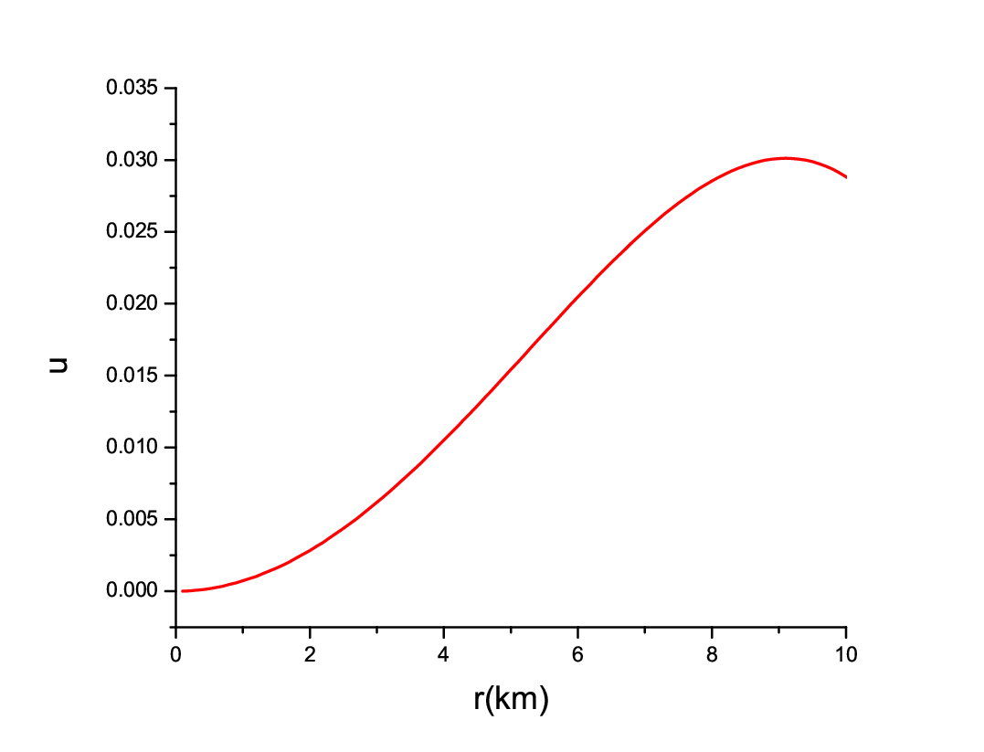
The surface redshift ( $Z_{s}$ ) corresponding to the above compactness ( $u$ ) is obtained as

1+Z_{s}=\left[1-(2u)\right]^{-\frac{1}{2}},

(23)

where

Z_{s}=\frac{1}{\sqrt{1-\frac{b^{2}}{R^{2}}+4\frac{b^{4}}{A^{4}}}}-1

(24)

Thus, the maximum surface redshift for the anisotropic strange stars of different radius could be found very easily from the Fig. 10. We calculate the maximum surface redshift for our configuration using the numerical values of the parameters as $b=9.5,R=16.9,A=24.18$ and we get $Z_{s}=0.375$ . The nature of surface redshift of the star is shown in Fig. 10.

IV Conclusion

In this work we have investigated the nature of anisotropic strange stars in the low-mass X-ray binary 4U 1820-30 by taking following considerations : (a) The stars are anisotropic in nature i.e. $p_{r}\neq p_{t}$ . (b) The space-time of the strange stars can be described by Tolman VII metric.

The results are quite interesting, which are as follows: (i) Though the radial pressure $(p_{r})$ vanishes at the boundary $(r=b)$ , tangential pressure $(p_{t})$ does not. However, at the centre of the star, it’s anisotropic behavior vanishes. (ii) Our model is well stable according to Herrera stability condition [17]. (iii) From mass-radius relation, any interior features of the star can be evaluated.

Therefore, our overall observations of anisotropic strange stars under Tolman VII metric satisfies all physical requirements of a stable star.
It is to be noted that while solving Einstein’s equations as well as for plotting, we have set c=G=1. Now, plugging G and c into relevant equations, the values of the central density and surface density of our strange star turn out to be $\rho_{0}=0.55~\times~10^{15}~gm~cm^{-3}$ and $\rho_{b}=0.27~\times~10^{15}~gm~cm^{-3}$ for the numerical values of the parameters as $b=9.5,R=16.9,A=24.18$ . Also, the mass of our strange star is calculated as $1.01M_{\odot}$ . Interestingly, we observe that the measurement of the mass, radius and central density of our strange star are almost consistent with the strange star in the low-mass X-ray binary 4U 1820-30 [22].

Recently, Cackett et al. [23] reported that the gravitational redshift of strange star in the low-mass X-ray binary 4U 1820-30, based on the modeling of the relativistically broadened iron line in the X-ray spectrum of the source observed with Suzaku is $Z_{s}=0.43$ . The surface redshift of our strange star with radius $9.5$ km turns out to be $0.375$ . This indicates that the measurement of redshift of our strange star is nearly reliable with the strange star in the low-mass X-ray binary 4U 1820-30.

Finally, we conclude by pointing that spacetime comprising Tolman VII metric with anisotropy may be used to construct a suitable model of a strange star in the low-mass X-ray binary 4U 1820-30.

Acknowledgments

MK, FR and SMH gratefully acknowledge support from IUCAA, Pune, India under Visiting Associateship under which a part of this work was carried out. FR is also thankful to UGC, for providing financial support under research award scheme. We are grateful to the referee for his valuable suggestions.

References

[1] Richard C. Tolman, Phys. Rev., 55, 364 (1939).
[2] F. Rahaman et al., Gen. Relativ. Gravit. 44, 107 (2012).
[3] F. Rahaman et al., Eur. Phys. J. C 72, 2071 (2012).
[4] M. Kalam et al., Eur. Phys. J. C 72, 2248 (2012).
[5] Sk. M. Hossein et al, Int. J. Mod. Phys. D 21, 1250088 (2012).
[6] M. Kalam et al., Int. J. Theor. Phys. 52, 3319 (2013).
[7] M. Kalam et al., Eur. Phys. J. C 73, 2409 (2013).
[8] F. Lobo, Class. Quantum. Grav. 23, 1525 (2006).
[9] K. Bronnikov and J.C. Fabris, Phys. Rev. Lett. 96, 251101 (2006).
[10] E. Egeland, Compact Star, Trondheim, Norway (2007).
[11] I. Dymnikova, Class. Quantum. Gravit. 19, 725 (2002).
[12] R.L. Bowers and E.P.T. Liang, Astrophys. J. 188 657 (1974).
[13] R.Ruderman, Rev. Astr. Astrophys. 10, 427 (1972).
[14] A.I. Sokolov, JETP 52, 575 (1980).
[15] H. A. Buchdahl, Phys. Rev., 116, 1027 (1959)
[16] J. P. de León , Gen. Relativ. Grav., 25, 1123 (1993)
[17] L. Herrera , Phys. Lett. A, 165, 206 (1992)
[18] H. Abreu , H. Hernandez and L. A. Nunez , Class. Quantum. Grav., 24, 4631 (2007)
[19] M. K. Mak , P. N. Dobson and T. Harko , Europhys. Lett., 55, 310 (2001)
[20] Stella et.al, ApJ,315,L49(1987).
[21] T.E.Strohmayer and E.F. Brown, ApJ,566,1045(2002).
[22] T. G $\ddot{u}$ ver et. al, ApJ,719, 1807(2010).
[23] E.M. Cackett, et al. 2008, ApJ, 674, 415