Charge-density-wave order with momentum and within the spin-fermion model: continuous and discrete symmetry breaking, preemptive composite order, and relation to pseudogap in hole-doped cuprates
Abstract
We analyze charge order in hole-doped cuprates within the the spin-fermion model. We show that magnetically-mediated interaction, which is known to give rise to -wave superconductivity and charge order with momentum along zone diagonal, also gives rise to charge order with momenta and consistent with the experiments. We show that an instability towards with or is a threshold phenomenon, but the dimensionless spin-fermion coupling is above the threshold, if the magnetic correlation length exceeds a certain critical value. At a critical , the onset temperature for the charge order terminates at a quantum-critical point distant from the magnetic one. We argue that the charge order with or changes sign under , but . In real space, such an order has both bond and site components, the bond one is larger. We further argue that and are not equivalent, and their symmetric and antisymmetric combinations describe, in real space, incommensurate density modulations and incommensurate bond current, respectively. We derive Ginzburg-Landau functional for four-component order parameters with or and analyze it first in mean-field theory and then beyond mean-field. Within mean-field we find two types of CDW states, I and II, depending on system parameters. In state I, density and current modulations emerge with the same or , breaking lattice rotational symmetry, and differ in phase by . The selection of or additionally breaks time-reversal symmetry, such that the total order parameter manifold is . In state II density and current modulations emerge with different and the order parameter manifold is , where in the two realizations of state II corresponds to either lattice rotational or time-reversal symmetry breaking. We extend the analysis beyond mean-field and argue that discrete symmetries get broken before long-range charge order sets in. For state I, which, we argue, is related to hole-doped cuprates, we show that, upon lowering the temperature, the system first breaks lattice rotational symmetry () at and develops a nematic order, then breaks time-reversal symmetry at and locks the relative phase between density and current fluctuations, and finally breaks symmetry of a common phase of even and odd components of at and develops a true charge order. We argue that at a mean-field is smaller than superconducting , but preemptive composite order lifts and reduces such that at large charge order develops prior to superconductivity. We obtain the full phase diagram and present quantitative comparison of our results with ARPES data for hole-doped cuprates.
I Introduction
Intensive experimental studies of hole-doped cuprates over the last few years have provided strong indications that the pseudogap region is a state (or even a set of states) with broken symmetry. First, X-ray and neutron scattering data on La1.875Ba0.125CuO4 strongly indicate [1, 2] that lattice rotational symmetry is broken from down to below a certain temperature . Evidence for rotational symmetry breaking has been also found in neutron scattering data on YBCO (Ref. [3]) and in STM data on Bi2Sr2CaCu2O8+δ, at energies comparable to (Ref. [4, 5]). Second, measurements of the Kerr angle at optical frequencies detected a polar Kerr effect [6], and polarized elastic neutron scattering measurements detected an intra-unit cell magnetic order [7, 8]. The onset temperatures for the Kerr effect and for intra-cell magnetic order are not equal, but roughly follow the same doping dependence as . The most natural interpretation of these two measurements would be that time-reversal symmetry is broken, although the absence of a sign change of a Kerr signal under the change of the direction of the applied magnetic field raises a possibility that the Kerr effect may be a non-reciprocal phenomenon, in which case it should be associated with the breaking of mirror symmetries. Recent optical experiments in the terahertz regime has found [9] a non-zero linear birefringence, which was also interpreted as the result of the breaking of mirror symmetries and of lattice rotational symmetry. The temperature dependence of the onset of a linear birefringence in YBCO closely follows the one for Kerr signal.
Third, X-ray measurements on YBCO (Refs. [10, 11]), Bi2Sr2-xLaxCuO6+δ (Ref. [12]), and Bi2Sr2CaCu2O8+δ (Ref. [13]) detected a static incommensurate charge density-wave (CDW) order with momenta and/or , and was determined to be equal to the distance between neighboring hot spots –points where the Fermi surface (FS) intersects with the magnetic Brillouin zone boundary [12, 13]. The observed order is not long-ranged, but this well may be due to pinning by impurities [14, 15]. Earlier NMR measurements [16, 17] and more recent sound velocity measurements [18] in a magnetic field found a true CDW order at . Quantum oscillation measurements [19] and measurements of Hall and Seebeck coefficients [20] were interpreted as feedbacks effect from the CDW order on fermions. The onset temperature of the CDW order was found to be smaller than but follow a similar doping dependence. Fourth, ARPES measurements deep under the superconducting dome have found [21, 22, 23] a change of system behavior at a certain doping, and were interpreted as evidence for the existence of a quantum-critical point (QCP) at , at which a new order emerges. It is tempting to associate this emerging order with CDW.
These and other experimental data [24, 25] pose a challenge to the theory. System behavior in the metallic region outside the pseudogap can be reasonably well described within a theoretical framework that fermions interact by exchanging quanta of collective excitations. One proposal along these lines [26], is that these excitations are charge fluctuations enhanced by phonons (a similar set of ideas has been recently displayed for Fe-pnictides [27]). An incommensurate CDW order with along or directions in the momentum space is a natural part of this scenario, and studies of a true and fluctuating CDW order within a microscopic Hubbard-Holstein model and using a more general reasoning of frustrated phase separation mechanism did indeed find [28] a CDW QCP at around optimal doping, identified the pseudogap temperature with the onset of CDW order [29] and obtained a number of features in Raman scattering [30], STM [31], and ARPES [32], consistent with the experimental data in hole-doped cuprates [33]. Furthermore, the residual momentum-dependent repulsive interaction mediated by charge critical fluctuations was argued to give rise to -wave superconducting instability, although additional interaction component, for fermions in antinodal regions, had to be included to match the experimental angular variation of the -wave gap [34]. An alternative proposal is that relevant collective excitations are spin fluctuations, peaked at or near antiferromagnetic momenta . The corresponding spin-fluctuation approach [35, 36, 37, 38] naturally explains -wave symmetry of the superconducting state and yields a non-Fermi liquid behavior of fermionic self-energy and optical conductivity [39, 40] in a rather wide frequency ranges, even when magnetic correlation length is only a few lattice spacings. This approach does describe precursors to magnetism [41, 42, 43] and accounts reasonably well for the phase diagram of electron-doped cuprates [44], where pseudogap behavior is very likely a crossover behavior due to magnetic precursors [45]. At the same time, until recently, spin-fluctuation approach was believed to be incapable to describe charge order and symmetry breaking in the pseudogap phase of hole-doped cuprates. Other explanations of charge order/symmetry breaking have been proposed, including loop-current order [46] or -density-wave (current) order [47, 48]. Other widely discussed scenarios of the pseudogap associate pseudogap behavior with precursors to either Mott physics [49, 50, 51, 52, 53], or superconductivity [54, 55, 56].
The spin-fluctuation scenario was revitalized by Metlitski and Sachdev [57] who found that the spin-mediated interaction is attractive not only in the -wave superconducting channel but also in the -wave charge channel, at momenta , where is the momentum of one of hot spot on a FS and are directed along one of Brillouin zone diagonals. In real space, an instability in a -wave charge channel implies a charge bond order, for which acquires an -dependent component of different sign for along and directions, while remains unperturbed. The analysis of CDW instability with within spin-fluctuation approach was extended by Efetov, Meier, and Pépin [58], who argued that the pseudogap behavior may be the consequence of the competition between bond order and superconductivity (in their scenario, the modulus of the combined SC/CDW “super-vector” order parameter emerges at but its direction gets fixed along the SC “axis” only at a smaller ). The “super-vector” scenario is appealing from theory perspective and allows one to explain some experimental data [59, 60]. However, it has three discrepancies with the experiments. First, the momenta are directed along one of the two Brillouin zone diagonals, while CDW momentum detected by resonant X-ray scattering [12, 13] and in STM [4, 5] is along horizontal or vertical axis in momentum space ( or . Second, bond-order instability is close to superconducting , but is below (Refs. [57, 58]), while experiments see the development of charge order above superconducting . Third, bond order with momentum does not break time-reversal or mirror symmetries and therefore does not explain Kerr, neutron scattering, and magneto-electric birefringence experimennts [6, 7, 8, 9].
In this paper we present a different scenario for the pseudogap due to spin-fluctuation exchange. We argue that magnetically-mediated interaction yields an attraction in the CDW channel for incoming momenta and , and, when magnetic correlation length is large enough, gives rise to a CDW instability at a nonzero temperature . That such critical temperature exists is not guaranteed a’priori, despite that, as we show below, there are logarithms in the perturbation theory. The reason is that magnetically-mediated interaction is dynamical, and the gap equation is an integral equation in frequency. For the latter, the summation of the leading logarithms does not necessarily give rise an instability [61, 62], and one one has to go beyond the leading logarithmic approximation to verify whether or not the interaction exceeds a certain finite threshold. We show that for CDW with or , the interaction is above the threshold, and the linearized gap equation, or, more accurately, the set of coupled equations for and , does have a solution at a finite . We compute first in Eliashberg-type calculations and then by treating the effects of thermal bosonic fluctuations beyond Eliashberg theory, and compare with obtained using the same procedures. In Eliashberg calculation, we show that and are finite at at . With more accurate treatment of thermal fluctuation (equivalently, the contribution from zero bosonic Matsubara frequency) we find that the ratio approaches one at infinite , i.e., and must be quite close at large . We also analyze non-ladder diagrams and show that they are small numerically.
The CDW order parameter changes sign under momentum shift by , as the bond order does, but it also has a non-zero on-site (a true CDW) component because . This agrees with the structure of the charge order extracted from STM and X-ray data [5, 63]. Because on-site component of is non-zero (albeit small) we will be calling this order a CDW, primarily to distinguish it from a true bond order with diagonal , for which, by symmetry, .
We analyze the structure CDW order in detail, first in mean-field approximation and then by going beyond mean-field. Within mean-field, we first assume that and are even functions in and discuss the interplay between CDW orders with and . The linearized equations for both CDW orders have solution at the same . What happens at a smaller depends on how the two orders and interact with each other. We show that the interaction is repulsive, i.e., the two orders tend to repel each other. If the repulsion is weak, the two orders appear simultaneously and with the same amplitude, and the system develops a checkerboard order. If the repulsion is strong enough, it becomes energetically advantageous for a system to spontaneously break lattice rotational symmetry from down to and develop CDW with only or . In the real space, such an order has the form of stripes, e.g., with . To understand which type of CDW order develops, we derive the Ginzburg-Landau action to order and analyze its form. We find that the repulsion is strong enough such that the system prefers to break symmetry down to and develop a stripe order. This is consistent with STM data [5]. A different scenario for CDW order with and has been proposed recently [64], in which CDW is induced by superconducting fluctuations. In that scenario, CDW emerges as a checkerboard order
We next take a more careful look at the dependence of on the center of mass momentum . CDW order with, say, can be constructed out of hot fermions with and (pairs 1-2 and 5-6 in Fig. 1). The CDW order parameters and are not identical because is not a reciprocal lattice vector. As a result, with generally has two components – one is even in and the other is odd (e.g., and , respectively). In contrast, for charge order with diagonal , only the even in solution is possible because the center of mass momentum is at ) or and and are equivalent points.
We show that the even component represents a variation of site and bond charge densities (a variation of the cite density is ), while the odd component represents a fermionic current This current gives rise to a non-zero orbital magnetic field and, by definition, breaks time-reversal symmetry (TRS). This, however, does not lead to orbital ferromagnetism as vanishes.
We compute for even and odd components and show that for the even component is larger, in agreement with Ref. [65, 66], but the one for the odd component is a close second. We derive the GL model for four CDW fields, , , , and . We argue that at low both density and charge components are generally non-zero, and the system develops a CDW order of one of two types, depending on the interplay between system parameters. We label the corresponding ordered states as states I and II, In the state I, density and current modulations emerge with the same (either or ) via a continuous second-order transition. Such an order spontaneously breaks lattice rotational symmetry down to , like in the case when only was set to be non-zero. The density and the current component with a given are both non-zero at low enough and the phase difference between them is locked at . The order parameter in this state breaks lattice rotational symmetry and symmetry of the common phase of the two order parameters, and breaks an additional symmetry by selecting the relative phase to be either or . It is natural to associate this additional symmetry with time reversal (TR), which is then explicitly broken in the state I.
In the state II incommensurate density and current modulations emerge with different via first-order transition. There are two realizations of state II: in the first all four CDW components are non-zero and have equal magnitudes, while relative phases between and and between and are, simultaneously, either or . This is a -symmetric checkerboard state with order parameter manifold , where is associated with TR. In the second realization, only one density and one current components are non-zero, e.g., and . Such an order breaks lattice symmetry down to , but does not additionally break TR symmetry because the phases of and are uncorrelated. The order parameter is again , with now associated with lattice rotational symmetry.
We extend the analysis of the Ginzburg-Landau (GL) action beyond mean-field by applying Hubbard-Stratonovich transformation to collective variables and analyzing the resulting action within saddle-point approximation, in close similarity to the analysis of the nematic order in Fe-pnictides [68]. We specifically focus on the state I, which in mean-field emerges via a continuous transition. We show that discrete symmetries get broken before long-range charge order sets in. We show that, upon lowering the temperature, the system first breaks lattice rotational symmetry () at and develops a nematic order. Below , becomes non-equal to (), while , i.e., density and current modulations do not develop, . Such a nematic order has been discussed in series of recent publications on the cuprates [69] and Fe-pnictides [68]. Then, at a smaller , another composite order parameter becomes non-zero (for the order with ), while still . Under time reversal, transforms into , hence this composite order breaks TRS. This order can be understood as the locking of a relative phase of and at or without the locking of the common phase of and . The emergence of a preemptive composite order which breaks time-reversal symmetry has been verified in Ref. [70] using a different computational technique. Finally, below the system breaks symmetry of the common phase and the system develops a true CDW order (a quasi-long-range order in 2D). Within our theory, we identify the temperatures and as the experimental pseudogap temperature .
The existence of the preemptive order is the crucial element in our scenario. Without it, CDW instability would be subleading to -wave superconductivity and to bond order with diagonal as in mean-field approximation both have larger onset temperatures than . However, superconducting order parameter and order parameter for bond charge order have only one, even in , component, and for these two there is no preemptive instability which would break time-reversal symmetry. Moreover, neither superconductivity nor bond order break symmetry. For bond order this is the consequence of the fact that bond orders with and only weakly interact with each other because in a fourth-order square diagram for the interaction term some fermions are necessary far away from the FS. As a result, the two orders appear simultaneously and form a checkerboard-type structure. If the system parameters are such that gets larger than the onset temperature for superconductivity/bond-order, the first instability upon lowering of is into a state with a composite CDW order with . Once composite order forms, it reconstructs fermionic excitations and tends reduce the onset temperatures for superconductivity/bond-order because composite charge order and superconductivity/bond-order compete for the FS. At the same time, a composite CDW order increases the susceptibility for the primary CDW fields and hence increases , much like a spin-nematic order in Fe-pnictides increases the Neel temperature of SDW order [68]. An increase of compared to the onset of superconductivity/bond-order becomes even stronger once we include into consideration 2D fluctuation effects because composite order only breaks discrete Ising symmetry, while near-degenerate -wave superconductivity and bond order form weakly anisotropic model, in which is strongly reduced by fluctuations from manifold.
The two transitions at and have been also found in the scenario [64] that CDW order is due to strong superconducting fluctuations, but in that case CDW order has only an even in component and there is no intermediate range where symmetry and/or TRS are broken.
We next consider doping evolution of and the interplay between charge order and superconductivity at various dopings. We argue that decreases when magnetic correlation length decreases and vanishes at some finite , setting up a charge QCP at some distance away from the magnetic instability (see Fig. 17(a,b)). A similar doping dependence holds for the onset temperature for bond order with diagonal , as we also demonstrate. The ideas about a non-magnetic QCP at around optical doping have been presented in earlier publications [71, 46, 72], in our theory we found such QCP in microscopic calculations. The onset temperatures of nematic and TRS-breaking composite orders follow the same doping dependence as . Within saddle-point Hubbard-Stratonovich theory, and merge with at some small below which the system undergoes a single first-order CDW transition [73]. Whether this holds beyond saddle-point approximation remains to be seen, but in any case near the critical , is higher than both and , and at larger dopings (smaller ) only superconducting order develops. The precise location of the CDW QCP will likely by affected by superconductivity, as it generally happens when one order develops under the umbrella of another [74, 75, 76].
We assume that charge QCP exists and combine the doping dependencies of , , , and into the full phase diagram, which we show in Fig. 17(c). We conjecture that the reduction of in the underdoped regime is primarily the result of a direct competition between superconductivity and composite CDW order, while a reduction due to fluctuations between superconductivity and bond order [58] plays a secondary role. We emphasize that in our model superconductivity and CDW order are produced by the same underlying spin-fluctuation exchange interaction, and in this respect they are, in the terminology of Refs. [77, 78], intertwined rather than competing orders. The situation is again similar to the one for underdoped pnictides where superconductivity and SDW orders are also intertwine orders as they originate from the same 4-fermion pair-hopping interaction [75, 76].
We compare our theoretical phase diagram with the one for hole-doped cuprates and present quantitative comparison of our theory with ARPES data, including Fermi arcs in the normal state [79] and the doping evolution of the spectral function at low , when the systems moves from a pure superconducting state into a state where superconductivity and charge order co-exist. We argue that the agreement with the data is quite good, but to describe the evolution of the ARPES dispersion along the cuts closer to zone diagonals one needs to go beyond what we did so far and solve for the CDW order parameter for rather far away from the mid-point between hot spots.
The structure of the paper is the following. In the next section we consider the model. In Sec. III we analyze the onset of CDW order with momentum and at near-infinite magnetic correlation length, when spin-fluctuation mediated interaction in the strongest and fermionic self-energy is large and cannot be neglected. We present our solution of the ladder set of equations for the CDW order parameter first to logarithmical accuracy and then beyond the logarithmical approximation. We show that the CDW problem belongs to a class of threshold problems, however the value of the coupling in our case is above the threshold. We compute first in Eliashberg-type calculations and then by treating the effects of thermal bosonic fluctuations beyond Eliashberg theory, and compare with obtained using the same procedures. We also analyze non-ladder diagrams and present non-linear equation for CDW order parameter. In Sec. IV we expand near the ladder solution, show that the solution corresponds to the minimum of the effective action within the CDW subset, and discuss the interplay between CDW and superconducting and bond-order instabilities. In Sec. V we discuss the structure of the CDW solution within mean-field approximation. We first approximate CDW order parameters by and in hot regions and analyze the interplay between CDW orders with and . We show that CDW order breaks lattice rotational symmetry down to and develops in the form of stripes. We then show that CDW order actually has two components, one is even under and the other is odd ( and , respectively). Both are fields, and the odd component changes sign under time-reversal. We derive GL functional for four coupled CDW order parameters , , , and and argue that either state I or state II is realized at low , depending on the interplay between the two input parameters. We show that in the state I, CDW order still breaks lattice symmetry down to , and, in addition, the phases of and differ by . The selection or breaks TRS. In Sec. VI we analyze GL action for the state I beyond mean-field, by introducing collective variables (bi-products of ) and search for non-zero expectation values of these variables within saddle-point approximation. We argue that CDW order develops in three stages, via two intermediate phases, one with pure nematic order and another with additional breaking of TRS. In Sec. VII we consider the interplay between composite CDW orders, a true CDW order, and superconductivity, and obtain the phase diagram of hole-doped cuprates as a function of hole doping whose increase we identify with the decrease of a magnetic correlation length . Here we show that , , and decrease with decreasing and vanish at (the same) finite setting up a CDW quantum-critical point at some distance from a quantum-critical point associated with the onset of a magnetic order. In Sec. VIII we compare our results with the ARPES data both above and below . We present our conclusions in Sec. IX. The discussion on several technical issues is moved into Appendices. For completeness, in Appendix F we also discuss the doping dependence of the onset temperature for bond order and the corresponding phase diagram.
In our consideration we approximate the electronic structure and collective spin excitations as two-dimensional, i.e., neglect fermionic and bosonic dispersions along direction. We believe that the essential physics is captured within 2D treatment, although a coherent interlayer tunneling maybe important for the stabilization of the stripe phase [80]. We also assume that near CDW instability the system remains a metal, albeit with strong incoherence caused by quantum criticality. A development of stripe CDW order from a quantum antiferromagnet in the strong coupling regime has been recently considered in Ref. [81].

II The model
We use the same spin-fermion model as in earlier studies of magnetically-mediated -wave superconductivity [35, 37] and non-Fermi liquid physics outside of pseudogap region[38, 57]. The model describes low-energy fermions with the FS shown in Fig. 1 and with 4-fermion interaction mediated by soft spin collective excitations peaked at or near . We focus on hot regions on the FS, for which shifting by keeps a fermion near the FS, and expand fermionic dispersion near a hot spot as , where is a Fermi velocity at a hot spot, is a deviation from a hot spot along the FS, and dimensionless specifies the curvature of the FS. The Fermi velocities at hot spots , and , in Fig. 1 are , , and . The amplitude of the Fermi velocity and the value of are the same at all hot spots. The effective 4-fermion interaction is mediated by soft spin excitations is
| (1) |
where , , are fermionic (bosonic) Matsubara frequencies, and
| (2) |
where the last term in the denominator is the Landau damping with the coefficient (Ref. [38]). The Landau damping contains the same as in (1) because Landau damping of collective spin excitations also originates from the spin-fermion interaction.
Following earlier works [38, 57, 58], we assume that the coupling is small compared to the Fermi energy and focus on instabilities which occur at energies well below and at , before the system becomes magnetically ordered. One such instability is towards a -wave superconductivity [35, 36, 37, 62]. It involves fermions from hot and lukewarm regions on the FS (with the self-energy and , respectively), and, taken alone (i.e., without competition with CDW order) occurs at , which is non-zero at all and interpolates between at large , with weak dependence on , (Refs. [62, 82]), and BCS-like result , at smaller , when dimensionless coupling is small (see panel b in Fig. 17). Another instability, considered in [57, 58], is towards a -wave charge bond order with diagonal momentum , where . This instability develops at , which is smaller than at any non-zero , although rather close to it at (Refs. [57, 58]). We analyze the form of in (see Appendix F) where we show that vanishes at a certain , when .
Our goal is to analyze another CDW channel, the one with momentum or . This pairing involves fermions from hot/lukewarm regions 1-2, 3-4, etc. in Fig. 1. The analysis of a potential CDW instability involving these fermions is a bit tricky, because fermions in the two regions connected by (e.g., regions 1-2 and 3-4 in Fig. 1) are different in the sense that parallel (antiparallel) velocities are () in the first set and () in the second. Accordingly, the CDW order parameter does not obey a particular symmetry relation under , and one has to solve the coupled set of equations for and .
In the next two sections we consider CDW instability with momentum along either or axis near the onset of SDW order, when the magnetic correlation length is near-infinite. We consider what happens at smaller later in Sec. VII. We perform our analysis in two stages. In the next section (Sec. III) we solve the set of linearized gap equations for and within the ladder approximation and show that this set has non-trivial solution at a non-zero . In Sec. IV we re-derive the same set by performing Hubbard-Stratonovich transformation from original fermions to bosonic CDW variables and show that diagrammatic ladder approximation is equivalent to saddle point approximation in Hubbard-Stratonovich approach. We expand around Hubbard-Stratonovich solution within the CDW subset and show that saddle-point solution is the minimum of the effective action, i.e., fluctuations around saddle point solution do not diverge. We then discuss the interplay between our CDW and superconductivity/bond-order. We argue that our CDW order and the other orders can be treated within a generic Ginzburg-Landau functional. Taken alone, each order is stable and is not destroyed by fluctuations. This internal stability implies that the system develops the order which sets up at the highest . At a mean-field level, , hence superconductivity develops first. However, we show in Sec. VI that composite CDW order develops at and this temperature well may exceed . Once this happens, composite charge order provides negative feedback on superconducting/bond order, reducing the corresponding mean-field onset temperatures, and gives positive feedback on which in some parameter range becomes larger than .
III The onset of CDW order with momentum and at
Borrowing notations from superconductivity, we will be calling the equations for and as “gap” equations. We will first solve for the onset of CDW instability in the ladder approximation without discussing its validity and later show that non-ladder contributions to the gap equation are small numerically. We start with hot regions 1-2 and 3-4 in Fig. 1. These two pairs forms a closed set for the CDW gap equations, and pairing in other hot regions should simply follow due to symmetry.
The gap equations in the ladder approximation are shown in Fig. 2. The CDW order parameters and are expressed via each other, and one needs to solve a set of two coupled gap equations to find an instability. Each equation is, in general, an integral equation in both frequency and momentum. Besides, fermionic propagators in the r.h.s. of the gap equations contain the self-energy which is large and depends on frequency and on the deviation of an internal fermion from a corresponding hot spot in the direction along the FS (Refs. [38, 57]). We present the calculation of in which we keep only frequency dependence in the fermionic self-energy and in the gap functions, i.e., approximate , when is near , and when is near . Such an approximation has been verified [62] to be a valid one the calculation of a superconducting and we expect it to be valid also for a CDW instability. The full gap equations, with momentum-dependent CDW order parameters and momentum-dependent self-energy are presented in Appendix A.
In analytical form the set of the two linearized integral equations in frequency for and is
| (3) | ||||
| (4) |
where , and are momentum deviations from the corresponding hot spots, , and the fermionic self-energy is the solution of the self-consistent equation
| (5) |
The fermionic Green’s function is related to as
| (6) |
where is fermionic dispersion which in Eqs. (3) and (4) we expanded around hot spots. For hot fermions in regions 1 and 2 in Fig. 1, is near , in which case .
At , the summation over frequency in (5) can be replaced by the integration. The equation for the fermionic self-energy becomes
| (7) |
One can easily make sure that at small enough frequencies. Earlier calculations [38, 57] of neglected self-energy in the r.h.s. of (7). In this approximation, the equation for is no longer of self-consistent form, and integration over and over yields
| (8) |
where . By order of magnitude, coincides with the spin-fermion coupling constant . For consistency with previous works, below we will use as the overall scale for the self-energy.
When the self-energy is kept in the r.h.s of (7) the self-energy at frequencies retains the same functional form as in (8), but with the extra prefactor
| (9) |
where, to a good numerical accuracy, .

To get an insight where the instability comes from, consider momentarily the case , . Then Fermi velocities at the two hot spots near (points 1 and 2 in Fig. 1) are antiparallel to each other, while the ones at the two hot spots near (points 3 and 4 in Fig. 1) are parallel. In this limit, Eqs. (3) and (4) reduce to
| (10) | ||||
| (11) |
In earlier large calculations of (Refs. [37, 38, 57]), the dependence of the bosonic propagator on the momentum transverse to the FS (i.e., the dependence in the last term in Eq. 10) and the dependence in Eq. (11) was neglected. If we used the same approximation here, we would obtain no CDW instability because the integral over in Eq. (10) would vanish. However, in our case the bosonic propagator does depend on and its poles are in both upper and lower half-planes of complex x. As a consequence, the momentum integration over in the r.h.s. of (10) gives a non-zero result even if we assume that Fermi velocities at points 3 and 4 in Fig. 1 are parallel. Furthermore, because at , , the poles in the bosonic propagator are located at comparable to that of the double pole. As a result, the result of the integration over is comparable to what one would get from integrating over in the two fermionic Green’s functions, if the poles there were in different half-planes of . In other words, the fact that the velocities at the hot spots at points 3 and 4 in Fig. 1 are parallel does not make the r.h.s. of Eq. (10) parametrically smaller compared to the case in Eq. (11), where the velocities at the two hot spots are anti-parallel and the momentum integral over the product of the two Green’s function already gives a non-zero result. In Eq. (11), the contributions from the poles in the Green’s function and in the bosonic propagator are of the same order and just add up in the overall prefactor.
We now return back to Eqs. (3) and (4) for and . We first integrate over in Eq. (3) and obtain
| (12) |
Introducing then and and using zero-temperature form of , we re-write (12) as
| (13) |
Integrating over in Eq. (4) and re-writing the result in the same variables and we obtain
| (14) |
The value of depends on the geometry of the FS. When Fermi velocities at hot spots 1 and 2 in Fig. 1 are nearly antiparallel, and the ones at hot spots 3 and 4 are nearly parallel, we have . When Fermi velocities at hot spots 1 and 2 are nearly perpendicular to each other, we have . For the FS as in hole-doped cuprates, is non-zero, but small numerically.
The negative signs in the right hand sides of (13) and (14) imply that the solution is only possible when and have opposite signs, i.e., CDW order parameter changes sign under . This does not imply, however, that the order has only a bond component (Ref. [57]). In our case, and differ in magnitude, and both on-site and bond components are present. For the on-site charge density we have
| (15) |
III.1 Gap equations to logarithmic accuracy
III.1.1 Neglecting frequency dependencies of and
As a first pass on Eqs. (13) and (14) we approximate gap functions as frequency-independent constants and , set the lower limit of integration over internal fermionic frequency to , and neglect the dependence on external frequency in (13) and (14). Evaluating the integrals with two fermionic and one bosonic propagators, we find that they are logarithmically singular, no matter what is. To logarithmical accuracy, we obtain
| (16) |
where
| (17) |
We emphasize that these two functions remain finite even if we set (i.e., set the velocities at hot spots 3 and 4 in Fig. 1 to be parallel to each other). Note also that and depend on the ratio of but not on , which cancels out between the overall factor in the spin-fermion interaction and in the Landau damping. This cancellation is typical for an instability mediated by a massless Landau-overdamped collective mode [82].

Evaluating and numerically, we found (see Fig. 3) that as long as . In the limit when (i.e., when the velocities at hot spots 1 and 2 are antiparallel, and the ones at hot spots 3 and 4 are parallel), we have and (). At non-zero , the values of and are closer to each other. That implies that the CDW order parameter in the region with nearly antiparallel Fermi velocities (region 1-2 in our case) is smaller than in the region with nearly parallel velocities (region 3-4 in our case). Solving the set (16) we immediately obtain that the linearized gap equation has a non-zero solution at
| (18) |
i.e., at . This is of the same order of magnitude as superconducting , which at the onset of SDW order is also of order (Refs. [37, 62]). Right at we have from (16)
| (19) |
III.1.2 Keeping frequency dependencies of and
Eq. (18) has been obtained within the approximations that (i) CDW order parameters and do not depend on frequency, and (ii) one can neglect the dependence on external in the r.h.s. of Eqs. (13) and (14). For a more accurate treatment, we need to keep the frequency dependence in and in .
Plugging Eq. (14) into Eq. (13) we get rid of and obtain integral equation for in the form,
| (20) |
where the kernel depends on both external and internal frequency.
We first analyze the pairing susceptibility. For this we add the source term to the right hand side of Eq. (20) and search for the divergence of at . At first order of iterations we replace by in the integral part and obtain . This is the same result as we had before, except for the additional factor which is due to the requirement that, when we compute , the internal frequency must be much larger than the external one in order to obtain correction. If subsequent iterations would transform into , as it happens in BCS theory, we would obtain similar to Eq. (18). However, we found that in our case the series of terms actually sum up into a power-law form . The implication is that, within the logarithmic approximation, the ratio does not diverge at any finite , i.e., Eq. (18) is an artifact of neglecting frequency dependence of . A similar situation holds in the superconducting channel. There, previous works have found [37, 62, 83] that the instability does develop, but to detect it one has to go beyond logarithmic accuracy, solve the full integral equation in frequency and search whether or not there is an instability at . This is what we do next.
III.2 Beyond logarithmic approximation
III.2.1 Pairing susceptibility at
The first step in the analysis is to consider , when the summation over Matsubara frequencies can be replaced by integration. At , the lower cut-off of the logarithm is set by frequency rather than by , hence within the logarithmic approximation
| (21) |
We now verify whether the actual pairing susceptibility at behaves similarly to (21) or changes sign, at least in some frequency ranges. The latter would indicate that that the normal state is unstable, hence is non-zero.
A similar strategy has been applied to superconducting problem at the onset of SDW order, when magnetic [37, 62]. We briefly discuss how it worked there and then apply it to our case. Like in our case, the summation of the leading logarithms for the superconducting problem does not lead to the instability and instead yields for the superconducting order parameter , where is again a source term and is some positive number of order one [84]. The solution of the full integral equation for at also yields a power-law form at , like in (21), however turns out to be a complex number. In this situation, there are two solutions, one with , another with . The linear combination of these two solutions yields oscillating
| (22) |
with a “free” phase variable . The presence of plays the crucial role when the analysis is extended to finite and the source term is set to zero. The power-law behavior at a finite exists in the frequency range between and and has to satisfy boundary conditions at the two edges. This requires two adjustable parameters. The temperature is one of them and the phase is the other one. Solving for the two boundary conditions requires care, but the result is that, very likely, they can be satisfied at a non-zero , i.e., at this the linearized gap equation has a solution. Whether this is the actual is a more subtle issue as there may exist some other solution of the linearized gap equation, with different behavior at small frequencies. In any case, however, the fact that Eq. (22) is the solution of the linearized gap equation at a finite implies that must be finite. From this perspective, the fact that the exponent is complex is a sufficient condition for the existence of the pairing instability at a finite in the quantum-critical regime.
We follow the same strategy for the CDW case. We keep the frequency dependencies of and in Eqs. (13) and (14), solve these two equations as integral equations in frequency, search for a power-law solution and analyze whether or not the exponent is complex. To shorten the presentation, we only consider the limiting case , and replace the soft upper cutoff at with a hard one. With this simplification, we obtain, replacing the sums by integrals
| (23) | ||||
| (24) |
We search for the solution in the form . One can easily verify that convergence of integrals requires . Substituting this trial solution into (23) and (24) we find after simple algebra a self-consistency condition
| (25) |
where is the universal dimensionless coupling constant for our quantum-critical problem and
| (26) |
We solved Eq. (25) for and found that the solution is a complex number: . The corresponding eigenfunction has the form , where is a free phase factor. Like we said, this is the sufficient condition for a CDW instability at a non-zero .
III.2.2 The computation of
Because the effective coupling is of order one, the only relevant energy scale in the quantum-critical regime is , hence must be of order . From this perspective, the estimate of in Eq. (18) is actually not far off as it also gives of order . To get the right ratio of , one need to solve the set of the two linearized gap equations numerically.
There is one caveat, however, associated with the special role of zero bosonic Matsubara frequency term in the gap equation. Indeed, the frequency sum in each of Eqs. (23) and (24) contains the term with . For this particular Matsubara frequency the integral over diverges logarithmically, as , and, if there was no counter-term, would vanish at .
This issue is known in the superconducting problem [37, 82, 61, 85]. The term with zero Matsubara frequency represents scattering with zero frequency transfer and a finite momentum transfer and from this perspective acts like an “impurity”. The logarithmical divergence of the integral over in (23) and (24) implies that “impurity” has an infinite strength at . Still, for an -wave superconductor, the contribution to from impurities must vanish by Anderson theorem. To see this vanishing in our formalism, one needs to do calculations more accurately than we did so far and re-evaluate fermionic self-energy at a finite , as it also contains a contribution coming from zero bosonic Matsubara frequency. For an -wave superconductor, the two contributions cancel each other. For other cases, the situation is less obvious. For -wave pairing, the divergent terms coming from zero bosonic Matsubara frequency do not cancel out within the Eliashberg approximation and this eventually gives rise to first-order superconducting transition [61]. For -wave pairing, earlier calculations within spin-fermion model used the Eliashberg approximation, in which the momentum integration is factorized – the one transverse to the FS is performed over the two fermionic propagators, while the one along the FS is performed over the bosonic propagator. Within this approximation, the contributions from zero Matsubara frequency to the pairing vertex and to the fermionic self-energy either completely cancel out in the gap equation [37, 85], when fermionic self-energy is approximated by its value at a hot spot, or the divergent terms cancel out and the remaining non-divergent terms give rise to a modest reduction of , when the momentum dependence of the fermionic self-energy on along the FS is kept (Ref. [82]). On the other hand, in our solution of the CDW problem, it was crucial to go beyond Eliashberg approximation and include the contributions from the poles in the bosonic propagator in the integration along and transverse to the FS. (We recall that, for interactions mediated by collective modes of fermions, there is no small parameter to justify Eliashberg approximation, except for special cases near three dimensions [86, 87]). To see whether or not the cancellation of the divergent contributions from zero Matsubara frequency holds in our case we have to keep the summation over Matsubara frequencies not only in the equations for but also in the self-energy. For definiteness, we consider the case , when Fermi velocities at one pair of hot spots are anti-parallel to each other and at the other are parallel. Like before, we neglect momentum dependencies of , and the fermionic self-energy, i.e., approximate these quantities by their values at hot spots. The inclusion of the dependence of the self-energy modifies Eqs. (23) and (24) to
| (27) | ||||
| (28) |
where , and
| (29) |
In (27)-(29) we used rescaled variables , , and . Let’s first analyze the equation for the self-energy . We recall that at we have . At a finite , the leading contribution to the sum in the r.h.s of (29) is from the term with . Restricting with only this term and neglecting bare (i.e., neglecting the difference between and ), we obtain from (29)
| (30) |
where . Solving (30) we obtain
| (31) |
where dots stand for terms of order one. This formula is valid when is a large number.
Substituting this into the first two equations and assuming that relevant and are of order one (we later verify this), we pull out and after integration over obtain
| (32) |
where . We see that, as long as we neglect non-logarithmic terms, . As a result, in this approximation CDW with has pure -wave form-factor and in real space represents a bond order, just like CDW with diagonal . A cite component (a true CDW) appears once we include corrections to (32) (labeled as dots in (32), and is small in . Such a structure of the charge order parameter is consistent with Refs. [65, 66, 67] and with the form of extracted from recent measurements [5, 63].
The reason why and become almost equal by magnitude in spite of the difference in the arrangements of Fermi velocities in regions 1-2 and 3-4 in Fig. 1 is that at large , the term in the fermionic propagator becomes larger than the term. Then the difference between nesting and anti-nesting becomes almost irrelevant as each fermionic propagator can be approximated by .
The r.h.s. of each of the two Eqs. (32) contains coming from in the denominator and the logarithmical term in the numerator due to the presence of zero bosonic Matsubara frequency term in the summation over . The logarithmical terms in the numerator and denominator exactly cancel each other, i.e., at this level there is no information what is. To obtain one has to keep terms with in the formulas for and for . We follow the strategy used in Eliashberg-type theories and introduce and . Substituting this into any of the two equations in (32) and using we obtain []
| (33) |
where we defined . The second term in the last bracket in the r.h.s. of this equation (the one with ) comes from the self-energy, once we express and in the l.h.s. of the two equations in (32) via . We see that term with zero Matsubara frequency vanishes, in agreement with what we found a few lines above (the term inside the parenthesis in the r.h.s. of (33) vanishes when ), and the value of is determined by the contributions from non-zero boisonic Matsubara frequencies. The vanishing of term is similar to what happens in an wave superconductor. However, contrary to an -wave case, here the effective coupling in (33) does depend on .
Eq. (33) has been studied in the context of color superconductivity [88] and of the pairing mediated by collective excitations in (Refs. [42, 70, 83, 86, 87]) and we just borrow the result: at weak coupling (small ) is determined by
| (34) |
Solving this equation, we obtain, in actual units
| (35) |
We see that thermal fluctuations reduce the CDW instability temperature by a factor compared to what we would obtain by using zero-temperature gap equation and just setting as the lower cutoff.
III.3 The interplay between and
There is another consequence of strong effect of thermal fluctuations – the onset temperature for CDW order with becomes almost indistinguishable from the onset temperatures for superconductivity and for bond order with diagonal . Indeed, the equation for superconducting is the same as Eq. (28) if we replace and . To logarithmic accuracy, this leads to the same gap equation for as Eq. (33). This is an expected result as superconducting problem and CDW problem with differ in the interplay between the directions of Fermi velocities in the two hot regions connected by . For superconducting problem the velocities at hot spots at and are strictly antiparallel, while for CDW they are almost antiparallel in one hot region and almost parallel in the other. In a situation when the frequency dependent term in the fermionic propagator becomes parameterically larger than , the difference in the directions of Fermi velocities becomes irrelevant and superconducting and CDW onset temperatures are both given by Eq. (35) to leading order in , and differ only in the subleading terms, which are small in , i.e.,
| (36) |
In real quasi-3D systems, the logarithm remains finite even when magnetic . In this situation, both and remain finite at the onset of CDW order (i.e., on a phase diagram they both cross line at finite ) and both are of order . Still, if is large enough, is close to , and the relative difference between the two temperatures is parametrically small in .

III.4 The role of non-ladder diagrams for
So far, in our consideration of the onset temperature for CDW instability, we analyzed the set of gap equations within ladder approximation, i.e., used the same type of diagrams as in BSC/Eliashberg theory of superconductivity, only in particle-hole channel. The ladder approximation is justified either at weak coupling, when the kernel in the gap equation is logarithmically singular and ladder diagrams contain higher powers of logarithms than non-ladder diagrams, or in the Eliashberg theory, when the coupling is not small but bosons, which mediate pairing, are slow modes compared to electrons. In this last case, non-ladder diagrams for the pairing vertex are small in Eliashberg parameter. Neither of this approximations can be justified in our case – the effective coupling is of order one and Eliashberg parameter is also of order one because the interaction in the CDW channel is mediated by collective modes of electrons, which have the same Fermi velocity as fermions themselves. Eliashberg parameter can be artificially made small by extending theory to large (Refs. [38, 57, 86]), but we do not use this extension in our analysis.
In the absence of any small parameter, non-ladder diagrams for the CDW order parameter are of the same order as the ladder ones, and one has to check whether they can significantly affect the result for . We do a simple check to verify this. Namely, we return back to the logarithmical approximation and check how much the prefactor of the logarithm obtained from one-loop ladder diagram changes when we include two-loop non-ladder diagrams. Specifically, we compare the prefactors from the two diagrams shown in Fig. 4. The one-loop diagram has been analyzed above, see Eqs. (16). To logarithmical accuracy it yields
| (37) |
where we used the fact that . For the case when Fermi velocities at hot spots 1 and 2 in Fig. 1 are anti-parallel, . For the same geometry the two-loop diagram in Fig. 4 yields, to logarithmic accuracy,
| (38) |
We see that the prefactor in Eq. (38) is ten times smaller than in Eq. (37), i.e., at least at this level of consideration, the two-loop non-ladder diagram in Fig. 4 only contributes a small correction to the one-loop ladder diagram. We take this result as an indication that the ladder approximation for the CDW order, while not justified parametrically, is reasonably well justified numerically.
IV The stability of the CDW solution
The existence of the solution of the gap equation for CDW order parameter by itself does not guarantee that there is an instability towards an CDW state. To prove that the system is truly unstable one has to verify that the solution with a non-zero CDW order parameter corresponds to a minimum of the Free energy, rather than a maximum. For a single order parameter , bilinear in fermionic operators a way to verify the stability is to use Hubbard-Stratonovich (HS) transformation, introduce as a real HS field, integrate out fermions, and expand the effective action in powers of . The expansion generally has the form
| (39) |
where and must be positive for a continuous transition. The saddle-point solution yields a conventional result . Expanding around saddle point to quadratic order in fluctuations and evaluating fluctuating contribution to the Free energy one finds that fluctuations increase and the Gaussian integral over fluctuations of nicely converges, i.e., the saddle point solution is a stable minimum. This simple reasoning, however, implies that . If was negative, saddle-point solutions with at and at would correspond to a maximum rather than a minimum of the effective action. One can formally convert these states into minima, but for this one has to transform the integration contour over from real to imaginary axis.
In our case there are two CDW orders, and hence one has to introduce two HS fields. We show below that the saddle point solution for is along real axis, while the saddle point solution for is along imaginary axis. Given that solutions along real and imaginary axis have very different physical meaning in the case of a single field, one has to perform a more detailed analysis of fluctuations around the saddle-point solution to verify whether in our case a disordered state is stable at and the ordered state is stable at .
Another complication in our case is associated with the fact that there are several directions of fluctuations around the CDW solution. The system can fluctuate in the CDW subset (i.e., within the plane set by and ), but it also can fluctuate in the directions of different orders, including superconductivity and bond order. All these fluctuations must be included in the full analysis of stability of CDW order [89].
We perform the stability analysis in several stages. First, we analyze the solution of the set of non-linear ladder equations and show that the mean-field solution with a non-zero appears continuously below . Then we analyze fluctuations around the mean-field solution in the and plane. Finally, we discuss the interplay with bond order and superconductivity.
To simplify the analysis, below we neglect the complications associated with the frequency dependence of and with pair-breaking effects of thermal fluctuations, i.e., approximate by as set as the lower cutoff of formulas. Within this approximation, . The inclusion of the frequency dependence of and thermal fluctuations will complicate the analysis but not change the conclusions.
IV.1 The non-linear gap equations at
The set of non-linear gap equations for CDW order with has been obtained in Ref. [90] and we reproduced their formula. For completeness, we briefly outline the details of our derivation. We again assume that Fermi velocities at hot spots 1 and 2 in Fig. 1) are anti-parallel, while the velocities of hot spots 3 and 4 are parallel. In regions 1 and 2 a non-zero acts in the same way as superconducting order parameter, i.e., is replaced by . In regions 3 and 4 a non-zero just shifts quasiparicle dispersions by , and the new fermionic operators which diagonalize the quadratic form, are and . In both regions we have normal Green’s functions of original fermions () and “anomalous” Green’s functions and . Combining the contributions to the ladder renormalizations of and from diagrams with two normal and two anomalous Green’s functions, we obtain, restoring momentarily the frequency dependence of :
| (40) | ||||
| (41) |
For definiteness, we set both and to be real.
At slightly below , one can expand the r.h.s. of (40) and (41) in powers and . Approximating now by frequency-independent values and restricting with the logarithmic approximation, we obtain to order ,
| (42) |
where and . Eliminating from these equations we obtain
| (43) |
where
| (44) |
and
| (45) |
We see that , hence the CDW transition is continuous.
IV.2 Fluctuations within the CDW subset
To analyze fluctuations within the CDW subset, we derive the effective action in terms of fields and , show that the saddle-point solution is equivalent to the solution that we found by summing up ladder diagrams, and then expand and around the saddle-point solution and analyze the stability of the effective action.
To make presentation easier to follow, we temporarily replace the actual momentum and frequency-dependent spin-mediated interaction by a constant . We restore the actual momentum and frequency dependence of the interaction in the final formulas for the effective action.
Consider for definiteness the ordering with , between regions 1-2 and 3-4. The 4-fermion interaction, which provides the glue for CDW, is
| (46) |
We define , and , and rewrite 4-fermion interaction as
| (47) |
The Free energy and the partition function is .
We use the HS identities [73, 91],
| (48) |
where ’s are in general complex fields, and apply these identities to and to decouple bilinear terms in in (47). The partition function is now and the action is now quadratic in fermionic fields. Integration over fermionic variables can be carried out explicitly and we obtain
| (49) |
We analyze the action in the saddle-point approximation and consider fluctuations around saddle point solutions. Because and couple linearly to and , non-zero saddle-point solutions for and/or imply that the corresponding and are also non-zero: and . In our notations then, and . (this does not mean that and are related by complex conjugation, since and are in general complex.) For our CDW solution , hence we expect non-zero saddle-point values of both and .
IV.2.1 Fluctuations at
We first consider the situation at , when we expect that the minimum of the effective action corresponds to . Integrating out fermions and expanding the result to quadratic order in and we obtain the effective action in the form
| (50) |
where
| (51) |
and
| (52) |
where the Green’s functions were introduced in (6). We show diagrammatic expressions for and in Fig. 5. The overall negative signs in Eq. (52) are due to the presence of fermion loops. Evaluating and , we find that they are both positive.

The action in (50) contains two terms with real prefactors of different sign ( and terms) and one term with imaginary prefactor. This apparently leads to some uncertainty as for a single field fluctuations described by converge if and diverge if . In our case, the prefactor for term is positive and the one for is negative, i.e, without the coupling provided by the term in (50) fluctuations of field would diverge. We will show, however that the term makes fluctuations of both and convergent at .
To prove this, we first notice that the effective action in (50) can be written in the form
| (53) |
Expressing complex and as , , where are all real, we re-write
| (54) |
as . Introducing then and as new variables, we find that integration over reduces to
| (55) |
This integral obviously converges. Integrating then over and before integrating over and we obtain that fluctuating part of the effective action reduces to
| (56) |
The prefactor is
| (57) |
The combinations and in the numerator have the same forms as the kernels in the gap equations for and . To see this we note that is the product of magnetically mediated interaction and two fermionic propagators with momentum difference . Restoring frequency and momentum dependence of and evaluating with logarithmic accuracy, we obtain
| (58) | ||||
| (59) |
Hence
| (60) |
Comparing this with Eq. (18) we immediately find that , and the prefactor is positive. This obviously implies that disordered state is stable at .
Another variable, whose fluctuations are convergent, is . The prefactor of the corresponding term in the effective action equals and remains positive at . Hence the combination , does not acquire a non-zero value even when becomes negative and the field condenses. Because , the condition together with yields
| (61) |
This is exactly the same as Eq. (19), which we obtained by summing up ladder diagrams.
We now pause momentarily and summarize what we just did. We re-expressed the effective action (50) as in (53), shifted variables and into the complex plane by adding to them and , respectively, and then integrated first over and along the direction parallel to real axis, and then over and . We found that all Gaussian integrals are convergent at , i.e., the disordered state appears as stable at .
We could, however, combine the three terms in (50) differently, by keeping as one variable and shifting by a term proportional to . This way, we re-write (50) as
| (62) |
Shifting now real and imaginary parts of by and , respectively, and integrating first over and parallel to real axis and then over and we obtain two divergent Gaussian integrals. Taken at a face value, this would imply that fluctuations of and diverge at , when . In reality, however, fluctuations do not diverge even if we integrate this way. To see this, one has to keep the limits of integration finite and set them to infinity only at the end of the calculation. One can then explicitly verify that in this computational scheme the Gaussian integral with as in (62) yields the same result as we found before. Specifically, the integral , obtained by integrating over first, yields
| (63) |
If, instead, we integrate first over and then over , but each time will keep the limits of integration finite, from to , we obtain
| (64) |
In Fig. 6 we plot as a function of for a fixed set of . We see that has an oscillating component, but clearly tends to one when gets larger. The conclusion here is that, no matter in which the integration is done, the disordered state is stable at and becomes unstable at when changes sign.

We discuss additional technical aspects of the evaluation of the partition function for complex effective action in Appendix C.
IV.2.2 Fluctuations at
The HS analysis can be straightforwardly extended to , however to perform it we need to expand the effective action up to quartic terms. Applying HS transformation and expanding to fourth order in we obtain
| (65) |
The coefficients and are given by square diagrams made out fermions and are shown in Fig. 7. In analytical form,
| (66) |

The integrals and are evaluated in Appendix B using linear dispersion around hot spots. In this approximation, is negative and finite and . Expanding further the dispersion relation, we find that is also non-zero, but is smaller than . The discussion below does not rely on the precise numerical values of and , and we keep both and as finite.
Differentiating (65) with respect to we find from the relation , with the prefactor renormalized from by a non-zero :
| (67) |
Solving then the other saddle-point equation and using , we obtain
| (68) |
Restoring the frequency and momentum dependence of , like we did before, we immediately find that this set is analogous to Eq. (42), which we obtained by expanding in in the set ladder gap equations (it is important to keep for this comparison). The equivalence shows that the set of ladder gap equations is equivalent to saddle-point of the effective action.
We next replace in Eq. (65) by its saddle-point value and expand in powers of . We obtain
| (69) |
where, we remind, and
| (70) |
where, again, and hence, when is close to zero. Because is negative, is much smaller than , and is also small, it follows from (70) that , as expected. We verified that, if we restore the frequency and momentum dependence of , the order parameters and , obtained by minimizing (69) with respect to and using (67) to obtain , are equivalent to the solution of the non-linear ladder equations (43). Gaussian fluctuations around the HS solution can be obtained by usual means and indeed show that the saddle-point solution is a minimum with respect to variations of .
IV.3 The interplay between CDW order and superconductivity/diagonal bond order
So far, we considered only fluctuations within the CDW subset. The discussion in the preceding section shows that within this subset the CDW solution is is a local minimum and fluctuations are convergent. The order parameters and are proportional to each other and the effective action can be expressed in terms of one of them, which we label :
| (71) |
with and , .
There are indeed also fluctuations in the other directions, including the direction of -wave superconductivity and diagonal bond order. There fluctuations are longitudinal ones for CDW order and describe the change of when the magnitude of decreases and the magnitude of superconducting order of diagonal bond order increases. To describe these fluctuations we extend the GL expansion of the effective action to include the competing channels. To avoid complex formulas we only consider superconducting channel with order parameter .
A straightforward analysis shows that the full effective action has the form
| (72) |
where dots stand from higher-order terms, , and . The effective action of this form has been presented in Ref. [92]. The prefactor doesn’t have to be the same as for CDW order but can be adjusted to match that of by rescaling the magnitude of .
We know from the analysis in Sec. III that the instability temperature in the superconducting channel is close to , but still larger than (see Eq. (36)). Analyzing the effective action (72) within mean-field theory, we find that immediately below only superconducting order emerges, while CDW order emerges at a lower :
| (73) |
provided that two conditions are met[93, 75, 76]
| (74) |
The first condition makes certain that the mixed state has lower energy than either of the two pure states and the second one guarantees that . If any these two conditions is not met, the system remains in a pure superconducting state down to and CDW order does not develop.
We show below that beyond mean-field the situation is more involved and the first instability upon lowering can actually happen within CDW subset, before superconducting order or bond order with diagonal develop. The reason is that the manifold for the CDW order parameter includes one or two additional discrete symmetries, depending on the actual structure of the CDW order. We demonstrate this in Sec. V. In Sec. VI we show that composite charge orders, associated with there symmetries, develop at temperatures larger than . Given that is close to , the onset temperature for composite charge order likely exceeds . Once a composite orders sets in, it gives a negative feedback on superconductivity and reduces , and, at the same time, increases the susceptibility for the primary CDW order and hence enhances . It the enhanced becomes larger than the reduced , the same GL analysis as we just did below shows that is further reduced and whether it develops in co-existence of CDW at a lower depends on the same conditions as in (74).
V The structure of charge order: Mean-field analysis
In previous sections we considered CDW order with momentum either or and assumed that with a given is a single field, i.e., that .
In reality, the CDW order can emerge with either only or , or with both momenta, and also and are in general not identical because is not a high-symmetry point in the Brillouin zone. Indeed, by construction, the order parameter satisfies . This condition implies that an incommensurate charge order parameter has an overall phase factor associated with the breaking of symmetry, but does not specify how changes under . For set 1-2 and 3-4 in Fig. 1, relevant are near and . For the set 5-6 and 7-8 in Fig. 1, relevant are near and . As long as typical are smaller than (i.e., as long as is smaller than, roughly, ), the two regions are weakly connected and at zero-order approximation can be considered independent on each other, in which case the gap equation does not distinguish between the solutions for , which are even and which are odd under . One can easily check [65] that under time reversal , hence the odd in solution changes sign under time-reversal, and its emergence therefore implies that CDW order breaks time-reversal symmetry. We emphasize that the possibility to have two types of solutions is specific to CDW order with (). For a charge order with a diagonal , the center of mass momentum is at , and only an even in solution is possible.
We label the even in solution as and the odd in solution as . We will show later in this Section that in real space describes an incommensurate cite or bond charge density modulation, while describes an incommensurate bond current.
Combining two different with two components of for a given , we find that the full order parameter for CDW order has two components: , and . In this Section, we obtain the effective action for 4-component CDW order parameter and analyze it in the mean-field approximation. In Sec. VI, we preform the analysis beyond mean-field and study preemptive composite orders.
V.1 Truncated effective action: stripe vs checkerboard order

As a first pass on the structure of , we assume that has only an even-in- component (i.e., that ) and analyze the GL model for two-component order parameter and , subject to and . Our goal here is address the issue whether CDW order develops simultaneously with both and , in which case it preserves the underlying lattice symmetry and gives rise to checkerboard charge order in the real space, or with either or , in which case it spontaneously breaks symmetry down to and gives rise to stripe order The order with corresponds to CDW between fermions in regions 1-2 and 3-4 in Fig. 1 and the order with corresponds to CDW between fermions in regions 1-5 and 3-8. We introduce and as two HS fields, integrate over fermions, and obtain the effective action . The prefactors for and are identical by symmetry, and the full action to order is
| (75) |
Extending the result to fourth order in , we obtain
| (76) |
where, we remind, , . At a mean-field level, the effective action (76) gives rise to a checkerboard order when , and to a stripe order when . The coefficients and are expressed via the square diagrams with four fermionic propagators as
| (77) |
where is the ratio , which, we remind, is (see Eqs. (19, 61)). The terms are the convolutions of four fermionic propagators
| (78) |
We show graphically in Fig. 9, using the notations from Fig. 8. The overall minus sign in every line in (78) is due to the presence of a fermionic loop. The abbreviations for the Green’s function as , etc, and the integrals are performed over running frequency and momenta and . The integrals and have been already introduced in Sec. II.

We evaluate - in Appendix B, by expanding to linear order in the deviations from hot spots, and here quote the results. We obtain
| (79) |
Using these results we find that the prefactors and in Eq. (175) are given by
| (80) |
Because , we have at low , , i.e., the system chooses the stripe order in which only or emerges. Such an order spontaneously breaks lattice rotational symmetry.
Phenomenological arguments for stripe charge order in hole-underdoped cuprates have been displayed earlier [78], and our microscopic analysis is consistent with earlier works. We caution, however, that more accurate treatment is needed when CDW order emerges either from a pre-existing superconducting state, or in an applied magnetic field. Both a superconducting gap and a magnetic field cut the divergencies in and at low , and it may happen that in this situation becomes larger than , in which case the checkerboard CDW order develops.
V.2 The full effective action
We next analyze the effective action for the full 4-component CDW order parameter. We split into even and odd parts as
| (81) |
and, to shorten notations, define , , and as , , and , respectively. The four order parameters transform differently under translation along and directions in real space, lattice rotation by , and inversion of time. We list the symmetry properties of the four ’s in Table 1.
| Translation along | ||||
|---|---|---|---|---|
| Translation along | ||||
| lattice rotation | ||||
| Time reversal | - | - |
We again use HS transformation from the action written in terms of fermionic operators to the action in terms of collective bosonic variables and obtain the prefactors for quadratic and quartic terms in by integrating over the loops made out of two and four fermions, respectively. The full analysis is somewhat involved and to give insights what CDW configurations may emerge we first approximate the CDW order parameters by their values at hot spots, which in technical terms implies that we approximate vertices in the square diagrams for the prefactors for terms by their values at hot spots. Following the same steps as in the previous subsection, we obtain the effective action in the form
| (82) |
where , and . For , Eq. (82) reduces to (76) with . The expressions for are presented in (79). For these , all ’s are positive and and well exceed because corresponding are larger and also because is larger than one. The ratio of does not depend on and is given by . At low this ratio is large, but at it is generally of order one. To account for all possible phases, we will treat and as the two parameters of comparable strength, but will keep .
We parametrize the four fields , , and as
| (83) |
where all angles are taken between 0 and . Plugging this into Eq. (82) and varying over we find that the action is minimized when
| (84) |
This condition “locks” the phase difference between ’s and ’s for CDW order parameters along the two directions of to be simultaneously either or both . Plugging Eqs. (83, 84) back into Eq. (82) we obtain
| (85) |
where in the last line we have used the approximation .
The structure of the CDW order is now obtained by varying this action over , , and . We found two types of states, I and II, depending on the interplay between and (see 10).
For , we find that the minimum of corresponds to , and arbitrary . The implication is that CDW order develops either with or , i.e., is in the stripe form, like we found before. We see, however, that both and develop, in general, and the relative phase between the two is . We label this state as state I. The relative magnitude of and is arbitrary at this level of consideration, but we show in the next subsection that it gets fixed when we include the dependence of vertices.
For , the action (85) is minimized when and . In terms of ’s this implies and . We label this state as state II. The relative phases of and and of and are again fixed at either or (with the same value for and components), but the relative phase of and and the relative magnitude of and remain arbitrary at this level of consideration. We show in the next subsection that the relative magnitude gets fixed once we include the dependence of vertices, but the relative phase of and still remains arbitrary.
In the next two subsections we present a more detailed study on states I and II.

V.3 Properties of state I
Suppose for definiteness that the ordering is along , i.e., and become non-zero below . The corresponding from (82) is
| (86) |
As we already said, at this level, while the phase difference of and is locked to be , the relative magnitude of and can be arbitrary, only is specified by minimizing Eq. 86. In fact, in this approximation one can easily make sure that the fields and decouple – the first line in (86) exactly reduces to
| (87) |
One implication of this equivalence is that in the hot spot approximation the fact that the phases of and are locked at does not have a physical consequence in the sense that the parameter manifold is , where the two ’s are the two completely decoupled order parameters at and , and symmetry is for the choice between and , and there is no additional component associated with the two choices for the phase locking. However, as we will see below, the decoupling between and is the artifact of the approximation of by its value at . Once we go beyond this approximation, and become coupled and symmetry associated with the two choices of phase locking becomes physically relevant part of the order parameter manifold.
To account for the effects due to momentum dependence of we adopt a simple “toy model” approach and assume that odd and even components of behave near as
| (88) |
where is along direction. The correspondent momentum dependence then appears in the vertices in 2-fermion and 4-fermion loop diagrams for and terms. Re-evaluating the GL action with these vertices we obtain
| (89) |
where
| (90) |
Here and are GL coefficients in the approximation and the corrections and are given by
| (91) |
where the integration extends to a finite range around hot spots. Expanding in (91) in we obtain
| (92) | ||||
| (93) |
where . In Bi2Sr2-xLaxCuO6+y, (Ref. [12]) hence and . From Eq. (92) we then find that , i.e., the renormalized mean-field CDW transition temperature for the even component, is larger than that for the odd component . This agrees with Refs. [65, 66]. We note, however, that the two are still very close to the original because and are very small numerically. A complimentary approach how to go beyond hot spot treatment is presented in Appendix E. It also leads to . We also have
| (94) |
For , .
Analyzing the effective action (89) in the mean-field approximation we observe that a relative phase between and is locked at , like in the case of a constant . In other words, if is real, should be imaginary. From we obtain
| (95) |
Assuming that both orders are non-zero, we obtain from (95)
| (96) |
An elementary analysis shows that this solution is a minimum of the effective action when . In our case
| (97) |
i.e., this condition is satisfied. The temperature at which acquires a non-zero value is
| (98) |
Below this temperature both order parameters acquire non-zero values and the relative phase is either or . The broken symmetry in the phase when both and are non-zero is , where continuous corresponds to the common phase of and and Ising corresponds to the choice or for the relative phase.
What happens at lower depends on the sign of , and the two orders co-exist down to . Interestingly, when , there is another temperature
| (99) |
at which disappears and at smaller only is non-zero.
It is also instructive to re-write the effective action (89) in terms of the original CDW order parameters and at the hot spots. From Eqs. (81,88) we have and , which is the same relation as in the hot spot approximation. Plugging them into Eq. (89), we obtain,
| (100) |
For momentum-independent vertices, and decouple in the effective action (87). However, we see that the fields and now interact with each other. To make this more clearly visible, let’s neglect small differences between and and between and , but keep a larger difference between and . In this approximation, the effective action reduces to
| (101) |
This can be equivalently re-expressed as
| (102) |
The advantage of this last expression is that it clearly shows that, for , is reduced when and appear together, and and because then the last term in (102) becomes . At the same time, the prefactor for the “nematic” term is positive, which implies that and must be equal. This holds when and are orthogonal to each other.
V.3.1 Physical properties of the coexistence state
We now consider physical properties of the coexistence state, when both even and odd CDW order parameters are non-zero. The generic condition imposes the constraint that must be even in and must be odd in . We then re-express the at hot spots 1-2 and 3-4 as (for )
| (103) |
where and are numbers. This breaks time reversal symmetry because under time reversal transforms into . The choice of relative sign in (103) specifies one of two non-equivalent solutions which transform into each other under time-inversion. On the other hand, the parity is not broken as under parity operation transforms into . Note that the order parameter (103) is similar, but not equivalent, to incommensurate complex -density wave order proposed in [94, 95].
Converting to real space, we find that the term corresponds to an incommensurate modulation of local charge and bond density in direction
| (104) |
The term corresponds to an incommensurate bond current, which flows along direction and has incommensurate modulation in direction (see Fig. 11 (a))
| (105) |
Note that the bond current modulation is in anti-phase with the density modulation. An incommensurate bond current in turn creates an incommensurate magnetic field . This, however, does not lead to orbital ferromagnetism as the total magnetic field, integrated over the volume of the system, vanishes: . To be more precise, current lines have to close at the boundary of a sample, and it is natural to expect that they close through the regions of excess charge, as shown in Fig 11 (b). This gives rise to a set of loop currents with circulation along the same direction, which do create a uniform magnetic field. However, a uniform field scales as the area of the sample rather than its volume and vanishes in the thermodynamic limit. This is very different from triangular loop currents proposed in Ref. [46].
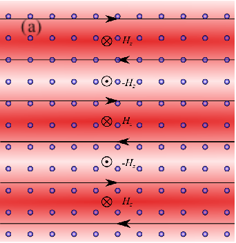

V.4 Properties of state II
We recall that in hot spot approximation, the minimum of the effective action, Eq. (85) for (state II) is at and , which in terms of ’s implies that and . The relative phases between and and between and are either both or . Substituting these relations into (85) and using and as two variables, we obtain the same effective action (86) as for the state I, namely
| (106) |
Like for the state I, the relative magnitude between and is not fixed in the hot spot approximation, and to find the actual CDW ordering one has to include the dependence of vertices. This gives rise to an effective action similar to Eq. (89), however for the state II the full effective action is more involved as all four CDW components are different from zero. We will not discuss the full form of the action because we believe that the state II is less relevant to the cuprates than the state I, and rather describe two potential realizations of the freezing of the relative magnitude of and , i,e., the breaking of the freedom associated with the realization of . One obvious choice is , another is , or , .
V.4.1 , ,
In this case all four CDW components, , , , , develop with the same magnitude . In real space this order corresponds to a checkerboard type incommensurate charge density modulation and incommensurate current in both and directions. We show this in Fig. 12 (a). The order parameter manifold is , where two continuous symmmetries are associated with the phases of and , and the Ising is associated with the relative phase between and , which is or , simultaneously for and components. This CDW order preserves lattice rotational symmetry but breaks time-reversal symmetry.
V.4.2 , ,
In this case, develops along direction and develops along direction, i.e., and . In real space this order corresponds to incommensurate charge density modulations in the direction and incommensurate current in direction. We show this in Fig. 12 (b). Such an order breaks two phase symmetries and breaks lattice symmetry down to such that the order parameter manifold is , where corresponds to . However the order parameter manifold does not has additional component, which one would associate with time-reversal symmetry, because only or appear along a particular direction of . Indeed, changes sign under time reversal, but this change is absorbed into phase symmetry.
The effective action for non-zero and is obtained from (82):
| (108) |
Because , the transition is again first order, into a state in which and have equal magnitudes.


VI Preemptive composite CDW order
We now go beyond mean-field theory and discuss potential preemptive transitions, when a discrete Ising symmetry gets broken at a higher than a continuous phase symmetry. We focus on the state I because in this state transitions are second order and the analysis of preemptive instabilities can be carried out within the GL expansion. This state is also more favorable for applications to hole-doped cuprates as phase transitions there are likely continuous ones. We will briefly discuss a potential preemptive order in the state II at the end of this section. We remind that the order parameter manifold in the state I is , where one is associated with the breaking of lattice rotational symmetry down to and another is associated with Ising symmetry breaking associated with the relative phase between even and odd in components of with a given . The lattice symmetry is broken by strong interactions ( and terms in the action), while associated with the relative phase is broken by weaker interactions, of order .
Below we discuss two preemptive composite orders associated with the breaking of each of the two discrete Ising symmetries without breaking of the phase symmetry. We analyze composite orders within “stage II” HS formalism, by which we mean that we introduce HS fields associated with composite orders, apply HS transformation to effective action written in terms of fields to decouple terms, integrate over fields and analyze the effective action for composite fields in the saddle point approximation. A similar procedure was applied in the study of a preemptive nematic order in Fe-pnictides [68] and of a preemptive translational symmetry breaking in doped graphene [91].
The saddle-point approximation for the action in terms of composite order parameters is valid when fluctuations around saddle-point solution are weak. This is the case when the number of components of the primary field field is large. The HS approach assumes that the original model can be safely extended to large number of field components in the sense that the results obtained in the controlled analysis at large are at least qualitatively correct for the original model with . We will perform large calculation below and show that composite orders associated with the breaking of each of symmetries in our case emerge at a higher than the one at which the primary field orders. A caveat here is that in 2D a primary field with does not order down to (Ref. [96]), hence a breaking of a symmetry at any non-zero is a preemptive order. Whether the actual system shows the same behavior depends on the type of the problem. For Fe-pnictides, the (magnetic) order parameter is a three- component unit vector, and it indeed does not order down to in 2D, like in large approximation. In quasi-2D systems, the primary field does order, but at a very low , which for weak coupling along the third direction is certainly smaller than a finite critical at which symmetry gets broken. In our case, however, the primary field is a two-component unit vector (a field), and the temperature at which the primary field orders in a quasi-2D system is finite and tends to Berezinskii-Kosterlitz-Thouless temperature in the 2D limit. Whether this temperature is still smaller than the one at which composite order develops is a’priori unclear and cannot be addressed within HS-based, large analysis. Fortunately, the emergence of preemptive composite orders has been verified within the approach specifically designed for a primary field [70]. We use the result of [70] as a verification that for the issue of a preemptive order a model with a two-component primary field is not qualitatively different from models with larger number of field components and proceed with the HS-based analysis.
VI.1 A nematic transition
We first discuss whether the breaking of lattice rotational symmetry down to can occur before the continuous phase symmetry gets broken. For this discussion, the presence of the two components of with a given does not play a role (the analysis of the truncated and full GL functional yield the same results with regard to breaking in the ordered state I). To simplify presentation, we then analyze the truncated GL functional with only component present. Our analysis of a preemptive nematic order will closely follow that in Ref. [68], but we also discuss the stability of the nematic phase.
The effective action for coupled order parameters and is presented in Eq. (76). Adding gradient terms and rescaling, we re-express (76) as
| (109) |
where, in comparison with (76), with , and . Because both and are positive and , we have . In principle, one should also include frequency dependence of the fields add the dynamical Landau damping term to , but to analyze the transition at a finite it is sufficient to consider only thermal fluctuations, i.e., the ones coming from .
We extend each field to components and re-write as
| (110) |
We introduce two HS fields: , conjugated to , and , conjugated to , as
| (111) |
Substituting these integrals into the the partition function and integrating over and , we obtain , where
| (112) |
The extremum of is obtained from and . This gives two equations
| (113) | ||||
| (114) |
The solution exists for an imaginary .
We follow Ref. [68] and introduce and . The primary fields get ordered when changes sign and becomes negative. This doesn’t happen in 2D, as long as . Replacing by , we obtain from Eq. (114):
| (115) |
VI.1.1 The solution
The set of equations (115) obviously allows a “trivial” solution . We have then
| (116) |
One can easily check the stability of this solution by verifying how the effective action changes when one moves along the trajectory which passes through a saddle point. For this implies shifting from along the real axis, for this implies shifting along the real axis from , where is the solution of (116). Introducing and , substituting into the action, and expanding to second order in and , we obtain
| (117) |
We see that the prefactor for is definitely positive, i.e definitely increases along the trajectory on Fig. 1. The prefactor for term is positive as long as . Combining this with Eq. (116), one finds that this holds when , where
| (118) |
The condition implies that , where .
VI.1.2 The solution with
Solving the set of saddle-point equations for , we obtain
| (119) |
where . The equation on takes the form
| (120) |
where, we remind, Expanding the l.h.s. of (120) at small , we obtain
| (121) |
We see that, if , gradually increases when becomes smaller than . To put it simply, the solution of the non-linear saddle-point equation shows that the order in emerges below , as it is expected for a continuous, second-order transition. We see the same behavior from Fig. 13 where we plot from (120) as a function of .

Let’s now see what we get if we expand near the saddle point solution. Introducing and , where, for definiteness, is the positive solution of Eq. (120), and expanding to second order in and , we obtain after a straightforward algebra
| (122) |
where
| (123) |
Obviously, , and are positive for .
Eq. (122) has the same form as Eq. (50) in the main text and Eq. (264) in Appendix F. Like we did there, we re-express in (122) as
| (124) |
The contour has to be chosen such that the variable is real, i.e we integrate over parallel to real axis.
As we already know, the condition that the saddle-point is the minimum of the action along the integration contour is . Substituting the expressions from (123), we find
| (125) |
where
| (126) |
The condition that the saddle-point is the minimum of the action along the integration contour is then . Expanding at small we obtain
| (127) |
We see that when . This is the same condition as in Eq. (121). One can easily verify that when , is positive for all values of .
VI.1.3 First-order transition at
For larger , the prefactors in (127) and (121) are negative. The analysis of the full saddle-point solution, Eq. (120) shows that, as gets smaller, the saddle-point solution (i.e., the solution of (120) first emerges at a finite , i.e., the transition is first order (see Fig. 14, in which we plot from (120) vs for .)

As gets smaller, two saddle-point solutions appear, one at , another at . By obvious reasons, the solution with is expected to be stable, while the one at is expected to be unstable. We see from Fig. 14 that the solution at corresponds to , and the solution at corresponds to . Now, evaluate
| (128) |
Comparing this with (126), we see that
| (129) |
Hence the solution with a positive corresponds to and is stable, as expected.
VI.2 Preemptive time-reversal symmetry breaking
We now return to the full GL model for and and consider a possibility of a preemptive breaking of symmetry associated with the relative phase, , between complex and . We recall that a nematic order is selected already within the hot spot model, while part of the order parameter manifold associate with phase locking becomes relevant only once we go beyond hot spot approximation and include the interaction between CDW order parameters and . Accordingly, the coupling constant associated with the nematic symmetry is larger than the one associated with the phase symmetry, and, hence , at which a nematic order sets in, is larger than a temperature, at which the other symmetry get broken. Still, it is essential to understand whether is larger than , i.e., whether symmetry associated with or gets broken at a temperature higher than the one when symmetry of the common phase gets broken.
We assume that nematic order selects, say, and consider GL model for and . A preemptive instability with respect to the relative phase of and would imply that at some and form a bound state with zero total momentum. In between and , , but becomes non-zero. Under time reversal, transforms into , hence this order breaks time reversal symmetry.
VI.2.1 Direct computation
One way to see that a preemptive transition is possible is to follow the same strategy as in the analysis of a spin-current order in anisotropic triangular antiferromagnets [97] and in Heisenberg-Kitaev model on a hyperhoneycomb lattice [98, 99], introduce a “two-particle” collective variable , and solve for the emergence of a two-particle bound state instability in the same way as it is done for superconductivity. For illustrative purposes we consider the effective action (86), although the actual calculation has to be performed for the more generic action (89) as we will do below using HS approach. We re-write (86) as
| (130) |
The ladder equation for is presented in Fig. 15 There are two terms in the r.h.s. of this graphic equation – the first contains a “direct” interaction from the first term in the second line of (130), and the second one contains the interaction between and . Both interactions are repulsive, hence no solution is possible if is real. However, if we search for a solution with a complex , we obtain for infinitesimally small
| (131) |
where stand for convolution of the propagators of and fields.

The only information about relevant to us at this stage is that it diverges at when both propagators become massless. Hence, if Eq. (131) has a non-trivial solution, the corresponding is larger than . A simple analysis of Eq. (131) shows that the solution does exist if we set to be purely imaginary, , because then the combination becomes equal to , and the minus sign compensates the overall minus sign in the r.h.s. of (131). We emphasize that this is possible because the prefactor for interaction term (the last term in (130)) is 4 times larger than the direct interaction term. That is purely imaginary is entirely consistent with the fact that in mean-field approximation is real and is imaginary, hence in below , is also purely imaginary.
VI.2.2 Hubbard-Stratonovich approach
Another way to see the emergence of a preemptive transition is to follow the same strategy as in the analysis of a pre-emptic nematic order and apply HS transformation to the effective action (89) by introducing collective variables conjugated to quartic terms in . For this purpose, it is convenient to rescale as , add the gradient terms and re-write Eq. (89) as
| (132) |
where , , where, we remind, and are (near identical) mean-field transition temperatures for even and odd in components of . Also
| (133) |
The prefactors for the two terms in (132) as well as the prefactors for and do not have to be equal, but this complication does not lead to new physics and we neglect it.
There are three quartic terms in (132). Accordingly we introduce three HS bosonic fields , congugated to , , congugated to , and , congugated to . The expectation value of each HS field is proportional to the corresponding bilinear combination of and . The field describes Gaussian fluctuations of the modulus of a two-component order parameter and its expectation value is obviously non-zero at any . The field describes fluctuations of a relative magnitude of and . For , order parameters and are non-equal and is non-zero at any , hence the expectation value of is also non-zero for all . The field is different from the other two because the expectation value of and hence of becomes non-zero only due to spontaneous symmetry breaking.
We assume, without going into details, that the model is extended to large , as in the case of a nematic transition, and analyze the effective action for composite HS fields within saddle-point approximation. A similar HS approach has been recently used to study TRS breaking in Fe-pnictides [100, 101, 102] We use, as before,
| (134) |
Substituting this transformation into (132) and performing Gaussian integration over the fields and we obtain the effective action in terms of collective variables , , and in the form
| (135) |
where .
We analyze in the saddle-point approximation, by solving the coupled set of saddle-point equations
| (136) |
where and .
Our goal is to verify whether a solution with emerges before the primary CDW order sets in. In our 2D case, the primary order sets in when , hence the emergence of at any finite will be a preemptive instability.
Introducing , , and , we re-write the last two equations in (136) as
| (137) |
Evaluating the integrals we obtain
| (138) |
( is arc-hyperbolic-cotangent of ).
The primary fields and get ordered when becomes equal to zero. We see from (137) that this only happens at . This is specific to and to systems with components, as we already discussed.
At high temperatures, , , hence . In this range, the physically meaningful solution of 138 is , . As temperature decreases, and decrease, while increases. Still, according to first equation in (138), remains larger than . Eventually, changes sign and becomes negative. The quantities and evolve as shown in Fig. 16. At finite but large negative , and are both large and Eqs. (138) simplify to
| (139) |
From the second equation we obtain . Plugging this back to both sides of the first equation and introducing we find, at ,
| (140) |
Solving this equation we obtain
| (141) |
Note that, because and are close to each other at large , the susceptibility of the primary fields is strongly enhanced. Still, , i.e., the primary order does not develop.

We now look at the first equation in (136). Evaluating the integral, we find that the solution with infinitesimally small emerges when
| (142) |
Using the second equation from (138) we re-write this as the condition on a critical ,
| (143) |
This critical is some positive number because and [see Eq. (97), is equivalent to ]. We next use the fact that monotonically increases as the temperature decreases. Hence, must reach at some finite , and below this temperature the expectation value of becomes non-zero. A non-zero in turn gives rise to a non-zero value of the composite order parameter .
In the consideration above we used the fact that , in which case the expectation value of is never zero (see Eq. (136)), and only field acquires a non-zero value due to spontaneous symmetry breaking. In general is non-zero and positive. However, we found earlier that it is quite small because both and are very close to the original , which, we remind, is a mean-field CDW transition temperature in the “hot spot” approximation, when and are equivalent fields. If we set , i.e., set , we immediately find from (136) that the field can also order only due to symmetry breaking. The self-consistent equations for and now have equivalent kernels, and which of the two acquires a non-zero value depends on the ratio . Like we just said, in our case, , hence field orders under proper conditions, but . In this situation, only first two equations (136) matter, and solving them we obtain that acquires a non-zero value when the two conditions are met:
| (144) |
Solving this set we obtain that, like in a more general case, a non-zero emerges at a negative but still finite
| (145) |
At larger negative , i.e., at smaller , a non-zero gives rise to a non-zero value of the composite order parameter .
When , or, equivalently, , the equations for and are identical, and one can immediately make sure that and in (136) can be cast as “real” and “imaginary” components of the “super-vector” . In the HS analysis, the magnitude of becomes non-zero at some finite , however neither nor order at any finite because of fluctuations between the directions of and of . In other words, in this situation, there will be no preemptive order which would break TR symmetry. This is entirely consistent with the fact that without distinction between different and , the effective action decouples between and , such that both orders appear simultaneously at . This last result shows that non-equivalence of terms, namely the inequality , is the necessary condition for the existence of a preemptive state with composite order which breaks TRS.
VI.2.3 Preemptive order for state II
Before we proceed with the phase diagram, we briefly discuss potential preemptive orders for state II. As we found in the previous Section, the CDW transitions into both versions of state II are first-order. In this situation, the analysis within the GL model is meaningless. One can still argue, though, that because order parameter manifold in the CDW-ordered state has additional component (ether or for the relative phase between and , depending on the realization of state II), there may be a preemptive transition into a state with a composite order parameter. However, to investigate this possibility, one has to go beyond GL expansion in powers of . We will not pursue this issue further.
VII The phase diagram
For the rest of the paper we focus on state I, for which phase transitions are continuous ones. To construct the phase diagram for state I, we first consider how evolves when hole doping increases and magnetic correlation length decreases. We found that at a finite , the scale serves as the lower energy cut-off for the logarithm, i.e., in (16) gets replaced by, roughly, . As the consequence, decreases with increasing and vanishes when , i.e. when the dimensionless coupling constant . We show this behavior in Fig. 17(b). The vanishing of sets up a charge QCP at some distance away from a magnetic QCP. The temperature at which composite nematic order sets in, and the temperature at which the preemptive TRSB order sets in, also gets smaller as increases. We analyzed the emergence of the composite and CDW orders at using the same approach as in Ref. [73] (this requires one to include the dynamical term into in equation (135)) and found that the three lines, , , and all terminate near the CDW quantum-critical point QCP 2, which actually becomes the point of weak first-order transition [73]. It is possible, although not proven yet, that a preemptive order survives down to , in which case QCP 2 splits into two or even three quantum-critical points. We show the behavior of , and in Fig. 17(b).
The behavior of is different from that of superconducting . The latter does not vanish at a finite and just interpolates between quantum-critical form at large and BCS form at smaller , when becomes a small parameter. This behavior of superconducting has been studied in Ref. [37] and we also discuss it in detail in Appendix F below.
Panels (a) and (b) in Fig. 17 show the onset temperatures for superconducting order and for CDW and composite orders, when the CDW and SC are considered independent on each other. In reality, charge and superconducting orders compete for hot fermions on the FS, and the competition implies that the order, which sets up first, tend to suppress the other one. In the spin-fluctuation approach, the value of is larger than , but the two are of the same order and comparable in magnitude The values of and are larger than , and we assume that at large , we have , i.e., the composite charge orders set up first upon the lowering of . The composite order suppresses and gives rise to a non-monotonic behavior of already in the paramagnetic phase. At the same time, it increases the correlation length for the primary CDW order parameter [68], i.e, the composite order tends to increase . At larger , then well may become larger than the reduced , in which case charge order develops prior to superconductivity. At the lowest , our calculations in Sec. IV show that CDW and superconducting orders co-exist. The phase diagram for state I is shown in Fig. 17(c). It has a number of features consistent with the experimental data on hole-doped cuprates. Namely, the theoretical phase diagram contains regions of SDW and -wave superconductivity, and also a region with a nematic order, a region where time-reversal symmetry is broken, and a region of a true CDW order. The CDW order at co-exists with superconductivity and terminates at a CDW quantum-critical point QCP 2, distinct from the magnetic quantum-critical point QCP 1. It is tempting to associate the line with the onset of nematic order seen in neutron scattering [1, 2, 3, 5] and in Nernst experiments [103], associate line with the onset temperature for the Kerr effect [6], intra-unit cell magnetic order [7, 8], the magneto-electric birefringence [9], and associate with the onset temperature of CDW order [10, 11, 12, 13, 16, 17, 18], perhaps pinned by impurities[14, 15]. In our model calculations, the nematic transition temperature is larger than the onset temperature for time-reversal symmetry breaking. In general, the two temperatures are comparable, and the position of and lines on the phase diagram may depend on the type of material. The association of with these three experiments requires care because, as we said in the Introduction, Kerr effect does not change sign in a magnetic field over (Ref.6) and linear birefringence is often associated with the breaking of a mirror symmetry rather than with breaking of time-reversal [9]. To address this issue in more detail one needs to study 3D systems, particularly the arrangements of the charge currents between neighboring layers.

VIII Comparison with ARPES data
In this section we discuss in some detail the comparison between our theory and ARPES data. The data on the fermionic spectral function in the pseudogap region all show [21, 104, 105, 106, 107, 79] that below a certain , the spectral weight in the antinodal regions transforms from the FS to high frequencies, and the FS looks like a set of four disconnected Fermi arcs. We show below that this is an expected behavior for a system with strong CDW fluctuations, but without a true CDW order.
A generic charge order with an ordering momentum introduces a new term into the Hamiltonian. Then fermions with momenta all become coupled. For commensurate , where and are integers, the “chain” of coupled momenta gets closed when after steps, for incommensurate it is not closed, but for practical purposes one can approximate by a close commensurate value. To diagonalize such a Hamiltonian one has to solve a -dimensional matrix equation [65]. The energy eigenstates with eigenvalues are linear combinations of the original fermions,
The ARPES spectral function measures the correlator of fermions and contains contributions from all eigenstates, with different weights
| (158) |
We keep the damping term finite to model the state in which CDW fluctuations are well-developed but a true CDW order does not yet occur [108].
We use this procedure to obtain the spectral function at , as a function of for “damped” stripe CDW order with either or . The position of the peak in this spectral function yields the location of the reconstructed FS in the CDW-ordered state, a gives a finite width to the peak. In a macroscopic system, there exist domains with stripes in both directions, and we assume that the measured ARPES intensity is the sum of for and .
We show our result for the photoemission intensity in Fig. 18. The Fermi arcs, terminating at hot spots, are clearly visible. The actual FS’s in the CDW-ordered state indeed cannot terminate inside the BZ, but other pieces of the FS have small spectral weights and are washed out by a finite . In the calculations we used the dispersion from Ref. [21]: , with , , , , and we took , slightly different from in [21], to get a commensurate instead of in [21]. We then used , and set .

The appearance of the arcs can be understood analytically. Consider and focus on the region around hot spot 1 in Fig. 8, with momenta near . One can easily verify that the most relevant momenta involved in CDW-induced mixing are and , since for the other momenta in (VIII) either the gap is smaller, or the states are away from the FS. The effective Hamiltonian can then be diagonalized by the standard Bogoliubov transformation. Defining , , , , and , with we obtain
where
| (165) |
The nergy eigenvalues are
| (166) |
the ARPES spectral function at is
| (167) |
The peaks in the momentum distribution curves are at , which correspond to . This condition defines a hyperbola in the momentum space around the hot spot 1, as shown in Fig. 19. The solid and dashed lines in this figure are the original FS and the “shadow” FS . At small , there is another part of the FS, to the right of point 1 in this figure, but for large enough , used in the plot, this part is pushed out the BZ boundary. The spectral weight along the red line in Fig. 19 depends on coherence factors and is much larger for the part which is close to the original FS than for the part close to the shadow FS. As a result, the only visible spectral peak at in the momentum space is along the former FS , and it effectively terminates at the hot spot, as in Fig. 19. The contribution from the domain with is obtained in a similar manner, and the full result is the spectral function with the largest intensity at four Fermi arcs, as in Fig. 18.
The Fermi arcs in the disordered CDW state and the Fermi pocket in the ordered CDW state, whose position and size are consistent with quantum oscillation measurements [19, 109] have been recently obtained in the analysis [110], similar to the one we presented here, but extended to the full Brillouin zone.

We next consider the dispersion along the BZ boundary in the antinodal (AN) regions. Experiments [21] performed on (Pb-Bi2201) have detected two prominent features: (1) upon cooling below about the same temperature where arcs appear, the measured dispersion evolves into a band which comes towards a FS and then moves away from the FS, (2) the momentum, at with the reconstructed dispersion has a minimum, shifts from to a larger value , (3) once the system is further cooled down below , a weak, “shoulder”-like peak in appears in the energy distribution curve at the binding energy . We find that all these features can be accounted for within our theory.
Because the features are at finite energy, we can safely neglect and compute ARPES dispersion assuming a true CDW order. However, we still need to consider two domains: domain I with CDW order with and domain II with CDW order with . For simplicity, we will assume both CDW gaps can be approximated by constants, in which case , with . Because typical energy scale for the fermionic dispersion in the AN region is much smaller than the bandwidth, we again can neglect high-energy electronic states. A simple analysis shows that for low-energy consideration it is sufficient to include three states with momenta . We show this in Fig. 20 (a) and 20 (b).
In domain I, the two states with momenta and cross at a small positive energy at , which is larger than the original simply because the distance between the two neighboring hot spots (one on top of the other) is larger than the distance between the two points and , at which the FS crosses BZ boundary. The energy of the state with momentum is much larger in this region, so we can further reduce the three-state system to a two-state system. The energy eigenvalues at the crossing point are . Once exceeds , one of the energies, , becomes negative, and the corresponding state becomes visible by ARPES. Evaluating at different , we find that initially follows the original dispersion and moves towards zero, but deviates from the bare dispersion as approaches , passes through a minimum at some finite negative energy, and then moves away from the Fermi level. We show this in Fig. 20 (a). The minimum of the reconstructed dispersion is right at , where the two unreconstructed states with momenta and cross. That the minimum of the reconstructed dispersion is at momentum larger than the original is consistent with the experiment [21]. One can easily make sure that the shift of the minimum to is the consequence of the fact that the momentum of CDW order is along or . If CDW order parameter was with along the zone diagonal, the result would be the opposite – the position of the local minimum would shift to a smaller momentum. This is yet another indication that CDW order does emerge with or rather than with the diagonal . Note in this regard that would remain equal to if the reconstruction of the fermionic dispersion was due to precursors of superconductivity.
We used the experimental value of meV, and set meV to match the energy of the local minima at at meV, as in [21].
In domain II, with CDW order with , two out of three states are degenerate, and we define . We also define . Solving 3-by-3 matrix equation on eigenvalues and eigenfunctions, we find that the dominant contribution to the spectral function comes from the peak at . The value of is positive for the set of parameters which we used. Because ARPES can only detect filled states, the peak at is invisible to ARPES. In other words, in the normal state, the full dispersion, measured by ARPES, comes from domain I.
Once superconductivity sets in at , electron and hole states get mixed up, and the system develops a shadow image of at a negative energy, at . The superconducting gap is rather small in Pb-Bi2201, hence the image is approximately at . We show this in Fig. 20 (b). The emergence of the new band below is again consistent with the experiment [21]. To match the measured position of the new band at around meV, we use experimental values of meV, meV, and set meV, larger than meV. This is consistent with theoretical and .
In Fig. 20 (c) we show the combined peaks from both domains. This is our theoretical result for the spectral function for comparison with ARPES. In our view, the theoretical spectral function is quite consistent with the data.

The above analysis is valid in the vicinity of hot spots. More efforts are needed to see whether our CDW order is compatible with ARPES along the cuts away from hot regions, particularly near zone diagonals. The data in these regions have been successfully fitted by the theory based on pair-density-wave scenario [111]. To compare with the data within our CDW scenario one needs to go beyond what we did so far and to solve for CDW order parameter outside hot regions. This would require full model calculations on a lattice.
IX Conclusions
The goal of this paper was two-fold. First, to understand whether spin-fluctuation approach, which describes -wave superconductivity and non-Fl physics in the normal state, also allows one to understand the development of charge order in hole-doped cuprates. Second, to study the structure of charge order parameter and potential preemptive instabilities which break discrete symmetries but leave a continuous phase symmetry intact. We argued that magnetically-mediated interaction gives rise to charge order with momenta and , as seen in the experiments. The critical temperature for the onset of the charge order is comparable to superconducting at large values of magnetic correlation length and the ratio tends to one at . At the same time, as decreases with increasing doping, the ratio decreases, and at some finite doping vanishes, setting up the second quantum critical point at some distance away from the magnetic one.
Our most significant observation is that CDW order parameter with a given , say, has two components, one () is an even function of the center of mass momentum , another (), is an odd function of . In real space, these two components describe, respectively, an incommensurate site and bond density variation , and an incommensurate current . We derived and analyzed the full GL functional for four CDW components , first in the mean-field approximation and then beyond mean-field. Within mean-field, we found two CDW states – state I and state II. Which of the two states is realized depends on the interplay between two system parameters, which are comparable to each other and which we only know approximately. The state I emerges via a continuous transition and is of stripe type: non-zero CDW components have either or . Both and are non-zero, and the relative phase between these two fields is locked at . The full order parameter manifold for state I is where one is associated with the choice between and , another with the choice between and for phase locking, and is the symmetry with respect to the common phase of and . To obtain a phase with this order parameter manifold it was essential to include the center-of-mass momentum dependence of for near the mid-point between neighboring hot spots.
For state II, the CDW order emerges via a strong first-order transition, and in the ordered state and . There are two realizations of state II and the choice is dictated by the interplay between parameters which become non-equal only due to dependence of . One realization is the checkerboard order (all four ’s are non-zero and equal by magnitude), another is a stripe state with only two non-zero components, say, and . For both realizations, the order parameter manifold is , where in the first realization is associated with the phase locking at between and (same locking for and components), and in the second is associated with the symmetry between choosing with or .
We focused on the state I because it emerges via a continuous transition and analyzed the GL action beyond mean-field. Our goal was to understand whether the two Ising symmetries can be broken at higher temperatures than at which symmetry gets broken. We used HS approach, introduced composite fields conjugated to composite order parameters, which order if the corresponding symmetry gets broken, integrated over the primary fields, and analyzed the resulting effective action for the composite fields. We found that each of degrees of freedom gets broken before a true CDW order sets in. We found that at a highest a nematic order sets in, i.e., the system selects or , while phase symmetry remains intact. Then, at , another symmetry gets broken, and the relative phase between and gets locked at or , while symmetry of the common phase of and remains unbroken. In real-space picture, below both density and current components fluctuate, such that , however their fluctuations are correlated, and is non-zero. Such an order breaks time-reversal symmetry. Finally, at , symmetry gets broken and a true CDW order sets in.
The existence of the preemptive order is the crucial element in our scenario. Without it, CDW instability would be subleading to -wave superconductivity and also to bond order with diagonal as in the mean-field approximation both have slightly larger onset temperatures than (). However, superconducting order parameter and order parameter for bond charge order do not break lattice rotational symmetry and have only one, even in , component. Accordingly, there are no preemptive instabilities for these orders. Because and are close to each other at large and , it is likely that they also exceed and , in which case the first instability upon lowering of is into a state with a composite CDW order. Once composite order forms, it reconstructs fermionic excitations and tends reduce the onset temperatures for superconductivity/bond-order because composite charge order and superconductivity/bond-order compete for the FS. At the same time, a composite CDW order increases the susceptibility for the primary CDW fields and hence increases , much like a spin-nematic order in Fe-pnictides increases the Neel temperature of SDW order [68]. An increase of and compared to the onset of superconductivity/bond-order becomes even stronger once we include into consideration 2D fluctuation effects, because near-degenerate -wave superconductivity and bond order form weakly anisotropic model, in which is strongly reduced by fluctuations from manifold.
The phase diagram resulting from our analysis is shown in Fig. 17c. It has numerous features consistent with the experiments on hole-doped cuprates. We performed a more detailed comparison with ARPES studies and found good quantitative agreement with the data.
Overall, we believe that the most significant result of our theory is that it shows that pseudogap physics can be well understood within the same spin-fermion model which was earlier shown to yield -wave superconductivity and non-Fermi liquid physics. We believe that, with our result, the spin-fermion model re-emerges as the strong candidate for the theoretical model for the cuprates.
Several issues are not covered by this analysis and are left for further study. One issue is the interplay between our spin-fluctuation scenario and the one based on microscopic analysis of charge fluctuations [28]. Another issue, specific to our model, is to what extend for a true CDW order and for preemptive transitions vary between different families of hole-doped cuprates. The third issue is the detailed analysis of the relation between our composite charge order which breaks time-reversal symmetry, and Kerr effect [6] and neutron scattering results from Refs. [7, 8]. And the fourth issue is the interplay between our incommensurate charge order and incommensurate pair-density-wave (PDW) order discussed in Refs. [77, 78, 111]. The two orders are “cousins” in the same way as SC and diagonal bond order are. Whether fluctuations between our CDW order and PDW order further complicate the phase diagram remains to be seen.
Note added (06/27/2014) The phenomenological GL model for PDW order parameter has been considered in a very recent preprint by D. Agterberg and M. Kashuap [115]. They introduced two order parameters with along and directions in momentum space, and argued that and are not necessary the same. The “cousins” CDW and PDW order parameters transform into each other by changing one into and replacing spin dependence for CDW into for PDW, but without changing the momentum. A cousin of our CDW order parameter with the enter of mass momentum is PDW order with the total momentum . The orders and are then cousins of our and , and the non-equivalence of and explored in [115] is the PDW analog of the non-equivalence between and , which we explored in this paper. Agterberg and Kashuap also identified an additional component of the order parameter manifold, associated with time-reversal symmetry, and argued that can be broken at a higher than the one at which a true PDW order develops.
IX.1 Acknowledgement
We thank Ar. Abanov, E. Abrahams, D. Agterberg, H. Alloul, P. Armitage, W.A. Atkinson, D. Basov, E. Berg, Ph. Bourges, D. Chowdhury, C. Di Castro, P. Coleman, A. Finkelstein, K. Efetov, R. Fernandes, P. Goswami, M. Greven, M. Grilli, M-H. Julien, A. Kapitulnik, B. Keimer, S. Kivelson, D. Le Boeuf, P. A. Lee, S. Lederer, H. Meier, E. Mishchenko, M. Norman, A. Paramekanti, C. Pépin, N. Perkins, D. Pesin, D. Reznik, S. Sachdev, D. Scalapino, J. Schmalian, S. Sebastian, O. Starykh, L. Taillefer, A. Tsvelik, P. Wölfle, and V. Yakovenko for fruitful discussions. The work was supported by the DOE grant DE-FG02-ER46900.
Appendix A Gap equations for momentum and frequency-dependent CDW order parameters
In this Appendix we present the full linearized equations for the CDW order parameters as integral equations in momentum and frequency. We measure frequency and temperature in units of : , , , and measure momentum in units of : . We recall that , where is spin-fermion coupling. We keep the momentum dependence of along the FS and neglect the momentum dependence transverse to the FS. We consider the FS geometry as in Fig. 1 and, to avoid too lengthy formulas, consider the limit when Fermi velocities at hot spots 1 and 2 are anti-parallel and the ones at hot spots 3 and 4 are parallel. In this limit, the momentum dependence along the FS is along axis for and along axis for . Integrating over momentum transverse to the FS we obtain
| (168) | ||||
| (169) |
where and . For the self-energy we obtain
| (170) |
The term numerator is even in and renormalizes the Fermi velocity. We follow the standard procedure and incorporate this term into the bare dispersion. The expression for is obtained from (170) by interchanging and .
For large , the dependence on momentum in the self-energy and in the CDW order parameters can be neglected, i.e., , , . In this approximation, Eqs. (168) - (170) reduce to Eqs. (3) - (5) from the main text. In general, however, the gap equations are integral equations in both momentum and frequency. Moreover, at deviations from hot spots 1 and 2 along the FS acquires an imaginary part, which is also odd in frequency: , where and are even functions of momentum and frequency. To match this behavior, also acquires an imaginary part, odd in frequency, but at deviations from hot spots 3 and 4 transverse to the FS: , where and are again even functions of momentum and frequency.
In the same approximation, the linearized equation for wave superconducting order parameter is
| (171) |
The equation for rescaled gap function for the most generic case, when (i) the gap depends on momentum along the FS and (ii) fermionic self-energy is not assumed to be larger than other terms in the pairing kernel, is
| (172) |
We see that the term with zero bosonic Matsubara does not cancel out completely. However, when is larger than other terms, the dependence of on and of on become weak, and Eq. (172) reduces to Eq. (33) in the main text.
Appendix B Evaluation of the terms
In this Appendix we evaluate the terms - , which we need to decide whether the system develops stripe or checkerboard order. Each is a convolutions of four fermionic propagators:
| (173) |
The abbreviations for the Green’s function are , etc, where and label hot spots in Fig. 1). The integrations are performed over running frequency and momenta and . We use Green’s functions for Free fermions and expand to linear order near hot spots. The Fermi velocities at relevant hot spots are , , and .
For we obtain
| (174) |
We keep the upper cutoff in the momentum integrals. i.e., integrate over a finite momentum range around hot spots. We will take the limit and . The ratio can, in principle, be arbitrary for , but is definitely large for . We will keep in our calculations.
Introducing the new parameters,
| (175) |
we re-write as
| (176) |
We separate the -integral into . For we obtain
| (177) |
Note that the original integrand is singular in the infra-red, so it is important to keep the temperature finite as a regulator of the singularity and set only at the very end of calculations. We will use the same procedure for the other integrals.
The contribution to from is
| (178) |
In the first line we used the fact that . As we see, both contributions are small in . The full result for is
| (179) |
For we have
| (180) |
We again separate the integral over as . This time, the integral over from to vanishes because the poles are all located in the same half plane. The integral also vanishes:
| (181) |
As a result, .
Now we turn to . We explicitly write it down as
| (182) |
As before, we write . We evaluate by extending the integral over onto the half plane where the integrand contains a single pole
| (183) |
We see that is logarithmically singular at . The other part, , is regular at . Therefore, to logarithmic accuracy,
| (184) |
Finally, for we have
| (185) |
The most straightforward way to evaluate this integral is to first extend both - and -integrations to infinite limits and then check how the results change when we restore finite limits of integration. To evaluate the integral in infinite limits, we introduce new variables and and re-express as
| (186) |
We see that diverges as . The divergence comes from momenta much smaller than , hence the prefactor for term does not depend on whether the limits of momentum integration are infinite or finite. Integration in a finite limits gives rise to corrections to (186) of order .
Appendix C On the stability of HS saddle-point in a complex plane
In the main text we discussed the stability of the mean-field CDW solution. We used HS transformation and obtained the effective action in terms of HS collective variables and , proportional to the two CDW order parameters and . We found that the saddle-point solution below is such that one variable is real and another is imaginary. Expanding near the saddle-point solution, we obtained the effective action which contains bilinear combination of fluctuations of and with imaginary prefactor. This form of the action persists also if we expand around at . The complex form of the action requires extra care when one analyzes the convergence of the Gaussian integrals over fluctuations of and
The same situation with two HS fields emerges in the analysis of a spin-nematic order in Fe-pnictides [68]. There, the solution of the saddle-point equations for collective nematic variables is again such that one variable is along real axis and the other is along the imaginary axis. When one expands next the saddle-point solution, one faces the same issue of convergence of Gaussian integrals, taken by shifting one of variables into a complex plane.
In this Appendix we discuss several generic issues, associated with the expansion near the saddle points in the complex plane and with the accuracy of using saddle-point approximation for HS fields. Specifically, we follow the suggestion put forward in Ref. [89] and consider the model with no momentum dispersion (formally, in dimension ).
In this case the partition function can, in certain limits, be evaluated explicitly with or without HS transformation. We use this fact to demonstrate that the computational procedure, which we used in the main text, yields the results identical to the one which one obtains in a direct integration over the primary fields.
We consider two extensions of the original bosonic model, which allow us to put the calculation of the partition function under control. One is the extension to large . It is obtained by extending the underlying fermionic model to fermionic flavors (for details see, e.g., Ref. [68]). The net result of such an extension is the appearance of the overall factor of in the effective action for bosonic variables. Another is the extension to the number of components of the bosonic fields to large . This gives rise to more complex form of the action as quadratic and quartic terms in bosons change differently. We argue below that HS transformation is useful in the large limit, while at large it is easier to evaluate the partition function by integrating directly over the original variables, without introducing HS collective variables. To put it differently, large and large limits are the two examples when one has to take care in choosing the variables whose fluctuations are weak. At large , fluctuations of the original bosonic fields around mean-field solution are weak and there is no need to perform HS transformation. If one does transform to HS fields, one finds that fluctuations of HS fields around their mean-field solution are strong. On the contrary, at large , fluctuations of the original bose fields are strong, while fluctuations of the HS fields around their saddle-point values are weak. In this limit, HS transformation and the subsequent saddle-point analysis of the effective action in terms of the HS fields are fully justified.
Which extension better describes the original model is a’priori unclear and requires complimentary analysis [68, 70], particularly in the cases when the analysis in terms of HS variables yields a preemptive transition into a state with a composite order. In principle, such a transition may exist only at large enough and disappear when is reduced to the original value of order one. At the same time, we are not aware of the examples when a composite order, detected in the model, extended to large , does not exist in the original model with .
C.1 The model with one real field
We assume that HS transformation from the original fermionic variables to collective bosonic variables is already performed and consider the action in terms of bosonic fields. As a warm-up, consider the effective action for one real single-component bosonic field :
| (187) |
The partition function is
| (188) |
At a mean-field level, at and at .
C.1.1 Large .
Consider first the extension of the model to large (large number of flavors of original fermions). This extension adds as the overall factor to the action [68]
| (189) |
We first compute the partition function directly and by using HS transformation to composite bose fields.
For and , the quartic term can be neglected and we immediately obtain
| (190) |
For and , we expand near and after simple integration obtain
| (191) |
(the overall factor comes from summing up contributions from positive and negative ).
The crossover between the two results for occurs in the range . In this range, more accurate analysis is needed to compute the partition function.
We now use HS transformation
| (192) |
Substituting this into (188) and integrating over , we obtain
| (193) |
So far, this is exact (the argument of the log is perfectly well defined for real ), and the integration over indeed gives the correct I, as one can easily check. However, the reason we use HS transformation is that we hope that the integration over the field can be done by expanding around a saddle point. Let’s see what we get if we do this.
First, let’s obtain the saddle-point solution. Differentiating from (193) over , we obtain
| (194) |
The solution is along the imaginary axis: . Introducing , we re-express (194) as
| (195) |
There are two solutions of this equation. For one, , for the other . At large positive , is obviously small and hence . Because never crosses zero (see (195)), only the solution with a positive is physically relevant. We have
| (196) |
Now let’s expand around this saddle-point. Introducting via and substituting into (193), we obtain, without making any approximation,
| (197) |
where
| (198) |
Then
| (199) |
where
| (200) |
So far, all transformations were exact. Now let’s see whether we can treat as small and expand near the saddle point. Let’s start with positive . At and we have and . Expanding in (200) to second order in , we obtain
| (201) |
The integral over in (200) is perfectly convergent, and evaluating it we obtain
| (202) |
which is the same result as in (190).
For (and, still, ) the situation is more complex as now and . Substituting these forms into (199), (200), and rescaling, we find
| (203) |
where in rescaled variables
| (204) |
and . The exponent comes from the saddle point and is the same as in (191). However, the prefactor cannot be obtained by expanding around the saddle point – we clearly see from (204) that typical are of order one, hence one cannot approximate the logarithmical term in the exponent in (204) by expanding to order . Rather, one has to evaluate the full integral. This shows that saddle-point approximation is only partially valid at large – the exponent in comes out right, but the prefactor cannot be obtained by expanding near the saddle point to order .
The integrand in (204) converges at , and the integral can be easily evaluated by closing the integration contour in the lower half-plane (, ). There is a branch cut along negative imaginary axis, at . Integrating over the boundaries of the branch cut we obtain after simple algebra
| (205) | |||||
Substituting this into (203) we obtain
| (206) |
This expression coincides with (191), as it indeed should.
The message from this analysis is that, at large , there is no advantage of using HS transformation and expanding around a saddle point – it is more straightforward to compute by directly integrating over and expanding around its mean-field solution along the real axis. For , one has to expand around the minimum of at a non-zero , and this expansion is controlled by . Still, one can get the correct result for even from HS analysis. The exponent at comes from the saddle point, but to get the prefactor right one has to do full integration, without expanding to quadratic order in the deviations from the saddle point.
C.1.2 Large .
Let’s now consider different extension of Eq. (187). Suppose that the field has components, and .
At large , it is convenient to rescale the prefactor for term to 1/M and analyze the action
| (207) |
The partition function is
| (208) |
As in the previous Section, we compute in two ways: (i) by directly integrating over and (ii) by using HS transformation
We begin with direct computation. Introducing M-dimensional spherical variables, one can re-write (208) as
| (209) | |||||
where is the area of a dimensional sphere with unit radius. At large , .
Because of prefactor in the exponent in (209), the integral over can be evaluated by expanding around the minimum of . The position of the minimum is at , where
| (210) |
Introducing and expanding around saddle point we obtain perfectly convergent integral over with in the exponent, which justifies the expansion. Evaluating the integral over and adding the contribution from the saddle point, we obtain
| (211) |
where . Note that only a portion of the exponential prefactor in (211) comes from the saddle point, another portion comes from (the area of dimensional sphere).
We next evaluate the partition function using HS transformation. Using a generic formula for for real :
| (212) |
applying it to and integrating over the components of the field, we obtain
| (213) |
The saddle point is at , where
| (214) |
Like before, we can re-write the equation for the saddle point as
| (215) |
where . This equation formally has two solutions, for one , for the other . However, only the solution with is meaningful because (i) at large positive , is small and and (ii) doesn’t change sign as a function of because is not a solution of (215).
Introducing and expanding the exponent around the saddle point we obtain
| (216) |
The integration is elementary and yields
| (217) |
Using Eq. (214) and the fact that , one can easily verify that the expressions for the partition functions obtained directly and using HS transformation, Eqs. (211) and (217), are identical.
The message here is that the partition function in the large limit can computed directly by integrating over field, but it can also be obtained by using the HS transformation and expanding around the saddle point. This expansion is perfectly well justified at large and, moreover, the exponent in in (217) contains the action taken right at the saddle-point. In the direct integration, the exponent in comes partly from the action at the minimum and partly from .
Note that in both calculations we computed the partition function by expanding around the extremal value of the action (first derivative of the action vanishes). In the direct integration over , the point for which is along the real axis, and the integration over fluctuations of is also along the real axis. Within the HS approach, the extremum of the action is along the imaginary axis, and by writing we shift the integration contour into the complex plane. For one-component model this is not a dangerous procedure as the only requirement on the integration over in the HS approach is that the integration contour should merge with the real axis at infinite . Still, the agreement between obtained via HS transformation and by direct integration over along the real axis tells us that the shift into the complex plane, used in the HS calculation, is perfectly legitimate procedure. For one-field case, there is little doubt that this is true, but we will see below that the analogy between direct and HS calculations helps us to justify the integration over HS fields over the contour in the complex plane in a more involved case of two bose fields.
C.2 The model with two order parameters
For definiteness, consider the two-field model discussed in Ref. [68] in connection with a preemptive spin-nematic order
| (218) |
where .
As before, we extend the model separately to large and to large .
C.2.1 Large .
The extension to large is straightforward – one just has to multiply the effective action in Eq. (218) by . We have
| (219) |
We begin with a direct computation of . Introducing and substituting into (219), we obtain
| (220) |
For and , the term in the exponent is irrelevant and we get
| (221) |
For negative and, again, , one can complete the square in the exponential term, introduce as a new variable, and integrate over in infinite limits. This yields
| (222) |
The exponent has a maximum at . Expanding near the maximum, we obtain
| (223) |
Evaluating then the integral over , we obtain
| (224) |
Now let’s see whether we can reproduce this result using the HS analysis. We use
| (225) |
Substituting these integrals into (219) and integrating over and , we obtain
| (226) |
where
| (227) |
The equations on the extremum of the action are
| (228) |
One obvious solution is , , where, like in the previous case,
| (229) |
and
| (230) |
Introducing and expanding around this saddle point, we obtain
| (231) |
where
| (232) |
For and , and . In this case, saddle point is a minimum along real and real . The effective action can be approximated by
| (233) |
Substituting this into the integral for and integrating over and over , we obtain
| (234) |
which coincides with (222).
For and , the situation is different. Now and the prefactor for the term in (231) becomes negative: . This obviously implies that the extremum at is a maximum rather than a minimum, and one has to search for a solution of the saddle-point equations with . Such solution is a “nematic” solution in the current nomenclature, although a true nematic order is indeed impossible in zero-dimensional case.
Expanding near and , we obtain,
| (236) |
where
| (237) |
where and is assumed to be small. As in the case of one field, we cannot expand under the logarithm as typical and are such that the argument of the logarithm is of order one. The integrals over and over are, however, fully convergent, and the integration can be performed in any order. We notice that the integrand vanishes for all large in the lower half-plane and integrate over by closing the contour in the lower half-plane of . There is again a branch but along the negative imaginary axis of . Closing the contour such that it doesn’t cross the imaginary axis of in the range where the branch cut exists, and integrating over , we obtain, after straightforward algebra,
| (238) |
In writing (238) we used the fact along the branch cut and . To leading order in we then have , such that in the exponent in (237) can be approximated by .
Integrating finally over in (238) and substituting the result into (236), we obtain
| (239) |
This is exactly the same result as Eq. (224).
Furthermore, can easily check that the direct calculation and the one using the HS transformation yield the same values of average quantities. In particular, the direct evaluation of
| (240) |
yields for and for . In both cases, calculations are under control at . The analysis based on HS transformation yields the same result. The crossover from small to occurs in a narrow range . In principle, one can compute in this range and obtain the full crossover behavior of and related quantities. This, however, requires more computational efforts.
The conclusion of large analysis is that we can reproduce the result for the partition function at large by using the HS transformation. At , to do so we need to expand near the “nematic” solution . Typical deviations from the saddle-point solution at non-zero are small in . We cannot expand under the logarithm in (237) because typical values of the argument are of order one, but the integrand, viewed as a function of , is nicely convergent and can be evaluated using standard means. Once we integrate over , the remaining integral over is a conventional gaussian integral with large prefactor in the exponent. Obviously, typical are of order and are small.
C.2.2 Large .
Let’s now extend the original model of two scalar field to the model of two component fields, and take the limit . We have
| (241) |
and
| (242) |
We again compute in two ways – directly and via HS transformation. We will see that HS approach is advantageous because the part of the action associated with the deviations from the saddle point contains large in the prefactor. At the same time, the action written in terms of and has cross-term with imaginary coefficient. The validity of the evaluation of the gaussian integral over fluctuations in this situation has been questioned in Ref. [89]. We will see that the computation of I by direct integration over and is free from such complications as the integrals do not have to be shifted from the real axis. We argue that the way how the gaussian integration has to be done in HS approach is set by the necessity to obtain the same I as in the direct calculation. In this respect, zero-D case is a blessing, as for any there is no way to check HS calculation by directly integrating over (the term contains components with four different momenta, subject to momentum conservation).
We begin with the direct calculation of . Using dimensional spherical coordinates for each of the two M -component fields, we re-write (242) as
| (243) |
where, as before is the area of a unit sphere in M-dimensions. At large , .
Introducing
| (244) |
we re-express as
| (245) |
Introducing and , we re-write Eq. (245) as
| (246) |
where
| (247) |
Because the exponent in (246) contains an overall factor of , we search for the extreme of at and . Differentiating over and over , we obtain
| (248) |
The second equation in (248) has two solutions: and . For the first solution we have from the first equation in (248) , where
| (249) |
(we recall that, by construction, ). For the second solution, we have
| (250) |
where . Obviously, the solution with a non-zero exists only for , when . At the critical value , .
We now expand the action near each of the solutions. Expanding near , we obtain
| (251) |
We see that the prefactor for the term is definitely positive, but the one for term may have either sign. The solution with is the minimum of the effective action in the region where . An elementary calculation shows that this holds when . We checked the second solution for these and found that it corresponds to the maximum of the action and is therefore irrelevant. Evaluating the Gaussian integrals over and over , we obtain
| (252) |
The case is more interesting for our purposes. Now the solution with becomes a maximum with respect to variations of , and we need to look at another extremal solution and . Expanding in and , we obtain
| (253) |
where
| (254) |
One can immediately make sure that
| (255) |
The integral
| (256) |
then perfectly converges, no matter in what order we integrate. There is indeed no need to shift the integration contour from the real axis. Integrating in (256), we obtain
| (257) |
Substituting this result into the expression for and multiplying the result by because there are two extremal points and and one has to expand near both, we obtain
| (258) |
This result is valid as long as exceed typical . The corresponding condition is .
We next compute by applying HS transformation. The computational steps are the same as at large , and the expression for is
| (259) |
where
| (260) |
The saddle-point equations have the same form as at large N: and , where
| (261) |
One solution is obviously
| (262) |
The other solution is
| (263) |
where is the same as the one introduced after Eq. (251).
For , one can easily show that the solution with corresponds to the minimum of . Expanding near this point and evaluating the (fully convergent) gaussian integrals over and over , we immediately reproduce Eq. (252).
For , we need to consider the second solution and expand around a non-zero and . There are two solutions: and . We expand near one of them, say, , assume that we are in the region where , and multiply the result by . Expanding near and , we obtain
| (264) |
where
| (265) |
One can immediately make sure that all three pre-factors are positive, but now
| (266) |
The quadratic form (refa71) has exactly the same form as the one in our analysis of the stability of the CDW solution, see Eq. (50) in the main text. Here, however, we have a benchmark – the result for must agree with Eq. (258).
We first follow the analysis in the main text and combine the last three terms in the r.h.s. of (264) in the same way as we did there, into
| (267) |
We then integrate first over by shifting the integration variable by adding an imaginary constant, and then over . Both integrals are fully convergent, and integrating over and and assembling the prefactors, we obtain
| (268) |
This is exactly the same result as Eq. (258). The agreement justifies the integration procedure we used in the main text. Like we said there, we could alternatively integrate over first by combining the last three terms in the r.h.s. of (264) into
| (269) |
and then integrate over . In this integration procedure both integrals are formally divergent if we integrate in infinite limits. However, as we said in the main text, if we integrate in finite limits and set the limit of integration to infinity only after the integration, we do reproduce the same result as in Eqs. (258) and (268).
The conclusion of large analysis is that it is perfectly legitimate to expand near the saddle point in which one variable is along the real axis and the other is along the imaginary axis, and the way to obtain the correct result is to combine variables such that we get two convergent integrals. Here we explicitly verified this by comparing the answer, Eqn (268), with the one obtained by integrating over real axis, without shifting the contour, Eqn. (258).
Another way to see that the integration around the saddle point in HS scheme is non-controversial is to consider the last three terms in the r.h.s. of (264) as a matrix and evaluate its two eigenvalues. This is a simple exercise, and the result is that both eigenvalues have positive real parts when , which implies that Gaussian integrals over fluctuations are convergent.
Indeed, in zero-D case there is no true nematic order. Still, the analysis in this Appendix shows that one can successfully apply the HS procedure and reproduce the exact results for the partition function by integrating in the near vicinity of the saddle point. The key message is that the need to integrate over fluctuations along the contour in the complex plane is not an obstacle – Gaussian integrals over fluctuations near the saddle point nicely converge.
Appendix D An alternative HS analysis, with saddle points along real axis
In Sec. IV.2 of the main text we represented the 4-fermion interaction in the CDW channel as in Eq. (47), i.e. as
| (270) |
In this Appendix we consider a more general representation
| (271) |
in which we initially treat and are arbitrary positive parameters. We see that we have two Hermitian interactions, the first one is repulsive and the second is attractive. We now introduce two HS fields and for these interactions and perform HS transformation. We introduce , and we use the same identities as Eq. (48),
| (272) |
All integrals converge along the real axis. We apply these identities to and and obtain the effective action
| (273) |
where contains the fermionic part of the action.
D.1 Fluctuations at
Now, let’s integrate out the fermions and expand the effective action in powers of and . To quadratic order in the HS fields we obtain
| (274) |
where and are defined in Eq. (52). We now choose
| (275) |
With this choice, the effective action becomes Hermitian and we the HS fields and decouple:
| (276) |
We see that the prefactor for is always positive, i.e. . Using this condition, we find the relation between the average values of and :
| (277) |
The prefactor for term becomes negative at , for which, in original parameters,
| (278) |
Restoring the frequency and momentum dependence of , we find the same CDW instability condition as in Eq. (60). One can easily make sure that Eq. (277) is also equivalent to the condition on , which we obtained by solving the linearized gap equations (16).
D.2 Fluctuations at
D.2.1 Near
Next suppose that we at a temperature and is small. In this range, the order parameter is also small, and one can restrict with only fourth-order terms in the expansion in powers of . Expanding in we ontain
| (279) |
We first find the modified relation between parameters and , which will keep as an extremum of the action and then show that this extremum is a local minimum. The need to modify ratio comes from the fact that in the CDW-ordered state fourth-order terms bring Gaussian corrections to quadratic terms in and . A simple experimentation shows that we need to keep as an extremum we need to choose
| (280) |
From the fact that we find that
| (281) |
One can straightforwardly check that this equation is consistent with Eq. (67).
Next we verify that and correspond to a local minimum of the effective action. We write down the effective action as
| (282) |
where is a number of order one. Expanding around
| (283) |
we immediately find that this solution is the local minimum of .
It we now neglect the non-critical fields and , we obtain the effective action in terms of the order parameter along the real axis. The action has the form
| (284) |
where and . This agrees with Eq. (69) (we recall that in (69)). If we wouldn’t neglect but rather integrated over it, (assuming that fourth order term is irrelevant) we obtained the same effective action as in (284) but with slightly modified prefactors.
D.2.2 Smaller temperatures, full non-linear analysis
When is not small we can no longer expand in . We go back to the original effective action Eq. (273)
| (285) |
where we defined , , and
Explicitly integrating out fermionic degrees of freedom we obtain
| (290) |
The summations over frequency and momentum are assumed.
Like before, we must tune and such that remains an extremum of the action, and then to show that this extremum is actually a local minimum.
First we differentiate the effective action with respect to , and we find,
| (291) |
where in the last line we have defined
| (292) |
Diagrammatically, and are nothing but the polarization bubbles with fully dressed normal and anomalous propagators. Imposing the condition on the extremum of the action, we obtain
| (293) |
which is to be compared with Eq. (199). Taking derivative with respect to , we find that the CDW instability sets in when
| (294) |
Next we show that is a local minimum. We define the real part and imaginary parts of and as
| (295) |
Substituting this into the action we obtain
| (296) |
Differentiating twice with respect to and using Eq. (294) we obtain
| (297) |
where
| (298) |
These two are given by the same square diagrams from Fig. 7, which we used before, but for the case when CDW order is already developed Evaluating the integrals we find that is positive no matter what is. The same holds for differentiation over . Hence, is a local minimum.
The rest of the analysis proceeds the same way as near . Namely, if we neglect , the effective action in terms of has a conventional form, and increases as decreases. This still holds even if we perform Gaussian integration over fluctuations of .
Appendix E An alternative method to go beyond hot spot treatment
In this Appendix we present a complimentary approach to go beyond hot spot treatment of the CDW order parameters and . The conclusion we reach here is the same – has a stronger instability. For GL coefficients in Eq. (89), this corresponds to . In the main text we assumed that even and off components of behave as and , respectively, along the direction of the center-of-mass momentum . Here we assume a more simple momentum dependence of and , namely, assume that the CDW gap is concentrated around anti-nodal regions, and even component is a constant and the odd component by a linear dependence on momentum in a hot region:
| (299) |
where is the center-of-mass momenta when connects two fermions right at hot spots. Obviously, and are symmetric and antisymmetric about the point, respectively. We approximate the interaction by a constant within some momentum window and and set it to zero outside this window. We then explicitly compute the eigenvalues for even and odd in solutions and compare them. The two eigenvalues are given by ( is for even solution)
| (300) |
where is the Fermi function. We set and and evaluated the two integrals numerically using the dispersion relation for (see Ref. [21]). In Fig. 21 we show our results for as a function of the size of the momentum window .

Appendix F Bond order with diagonal momenta

For completeness and for comparison with our results on CDW order with or , we also consider charge order with momenta , as depicted in Fig. 22. A charge order with diagonal momentum has been studied in Refs. [57, 58]. The critical temperature for the instability towards such order is exactly the same as superconducting if one neglects the curvature of the FS near the hot spots. The gap function for a diagonal charge order has a -wave structure , the same as a wave superconducting order parameter. A wave charge order does not create a charge density modulation , but it introduces modulations of the correlation function between neighboring sites:
| (301) |
where and are vectors along and directions, in units of interatomic spacing . A charge order of this kind is called bond order (Bo)
To obtain the onset temperature for BO, , and compare it with SC in the presence of FS curvature, we add to the spin-fermion action two infinitesimal vertices and , where stands for 2+1 momentum . These vertices gets renormalized by spin-fermion interaction, and the critical temperature ( or ) is obtained when the corresponding susceptibility diverges, i.e., the solution for fully renormalized or exists even when the bare vertices are set to zero.
The authors of [57, 58] have demonstrated that a superconducting instability and an instability towards bond order come from the fermions located in the same hot regions, only for bond order one of the regions is shifted by . The ladder renormalizations of and are shown in in Fig. 23, where the wavy line is the spin-fermion interaction. In analytical form we have, at the corresponding critical temperatures,
| (302) |
where the spin-fermion coupling and the dynamical spin susceptibility are defined in Eqs. (1) and (2) in the main text. The difference in the overall sign in the r.h.s is due to different Pauli algebra – for superconducting vertex , while for bond vertex . One can easily verify [57] that, if one neglects the curvature of the FS, one finds , and hence . In this approximation, the kernels in the two equations (302) become identical, hence, . Once the curvature of the FS is included, the degeneracy is lifted and . The reasoning is that superconductivity involves fermions with strictly opposite , and the momentum integration can still be replaced by the integration over , with a constant prefactor, even in the presence of the FS curvature. For BO, the relation no longer holds in the presence of the FS curvature, and this reduces the kernel in the Eq. (302) for .

Explicitly, expanding near a hot spot, we obtain
| (303) |
where and are momenta parallel and perpendicular to the FS, respectively, and is a dimensionless parameter characterizing the curvature of the FS. We will use dimensionless parameters
| (304) |
where is the magnetic correlation length, present in . The dimensionless coupling , dimensionless correlation length , and dimensionless FS curvature are three input parameters for the consideration in this Section. An additional parameter, set by the FS geometry, is the angle between Fermi velocities at hot spots separated by . To simplify the presentation, we assume that these two velocities are orthogonal to each other.
In this Appendix we follow earlier works [37, 38, 57, 58, 86, 112] and assume that the spin-fermion interaction can be well approximated by its value between fermions on the FS. Integrating over momenta transverse to the FS in the fermionic propagators, we obtain integral equations for and , which depend on frequency and on momenta along the FS. The equations are
| (305) | |||
| (306) |
where stands for and
| (307) |
F.1 and at the onset of SDW order,
It is convenient to introduce the set of rescaled variables
| (308) |
where was introduced in the main text. In these notations, the linearized gap equation for BO becomes
| (309) |
where the rescaled self-energy is[38, 57]
| (310) |
We verified, using the same strategy as in our earlier work [62] on superconducting at , that the leading contribution to the r.h.s of Eq. (309) comes from the region where and . In this region, the momentum dependence of is more relevant than its frequency dependence. Keeping only the momentum dependence in and introducing and , we re-write (309) as
| (311) |
For superconductivity, the same procedure yields
| (312) |
Comparing Eqs. (311) and (312), we find that extra terms in the logarithm in (311) make it smaller than the logarithm in (312), hence in the presence of a FS curvature gets smaller than . Specifically, the curvature term couples to and provides a soft upper cutoff to the integral over , at . At the same time, remains finite, no matter how large is. Indeed, at large we have . In other words, at , there is no threshold value of above which BO would not develop.
To check our analytical reasoning, we solved Eqs (305) and (306) numerically and obtained the same result, namely decreases with increasing but remains finite. We show the results in Fig. 24. We set , , and varied .

F.2 and at a finite
When the system moves away from the magnetic QCP, it eventually recovers a conventional FL behavior in the normal state. Indeed, as the correlation length decreases, becomes the upper energy cutoff for the pairing [38, 113]. Below this scale, the spin susceptibility can be treated as frequency-independent and the fermionic self-energy is linear in frequency:
| (313) |
In the last line we have defined . Plugging this into Eq. (305) for superconducting and using the condition that typical are all small in this limit compared to , we integrate over momentum and obtain
| (314) |
For superconducting we then have a conventional BCS-McMillan result [114]
| (315) |
Hence, as the system moves away from the QCP, it crosses over to a BCS behavior, and gradually decreases as decreases and gets smaller.
For BO, the gap equation in the rescaled variables becomes, in this limit,
| (316) |
where we defined
| (317) |
Typical are of order , and in the second term in the denominator we can safely replace by . We see that the curvature now appears in a combination with a constant term and provides a lower cutoff for the BCS-like logarithmic behavior. This is qualitatively different from the behavior at the magnetic QCP, where the curvature was coupled to the running variable . Because of the cutoff, the frequency integral in (316) no longer diverges at . Hence, at some critical , the linearized gap equation for BO vertex has a solution at . Setting in (316) and integrating over , we obtain the condition when :
| (318) |
Canceling out and integrating over frequency, we find
| (319) |
This defines a critical at which BO vanishes:
| (320) |
At smaller , the equation on only allows a trivial solution , hence BO does not develop at any .


To verify this, we solved for and numerically. We set and and varied . We found that superconducting crosses over to BCS behavior at small enough and that for BO there exists a critical at which . We show the results in Fig. 25.
Although the behavior of resembles that of for CDW order with , the physics behind the reduction of these temperatures with decreasing magnetic is different. For BO with diagonal , the reduction of compared to and its eventual vanishing is solely due to the FS curvature. If we set to zero, and remain identical at any . For CDW order with , the reduction and eventual vanishing of upon decreasing of is not related to curvature and holds even if we set curvature to zero. At a small curvature then, , but which temperature is larger at depends on numbers. We emphasize again in this regard that for CDW with the first instability upon lowering is at , towards the state which breaks an Ising symmetry. No such transition holds for BO with a diagonal .
F.3 Interplay between superconductivity and bond order
In Fig. 26 we present the phase diagram for the (artificial) case when the only two competing states are superconductivity and BO with a diagonal , i.e. when CDW order with is just neglected. Because is larger than , the leading instability upon lowering is always into a superconducting state, BO may appear only at a lower . At the same time, at large , by itself is reduced because over some range of the system fluctuates between superconductivity and BO [58, 65] (a light blue region in Fig. 26). The phase diagram in Fig. 26 is similar to that in Ref. [58], but differs in that in our analysis BO only emerges at , i.e., there exists a quantum-critical point towards BO (QCP 2) at some distance away from a magnetic quantum-critical point QCP 1.
References
- [1] M. Hücker, M. V. Zimmermann, G. D. Gu, Z. J. Xu, J. S. Wen, Guangyong Xu, H. J. Kang, A. Zheludev, and J. M. Tranquada, Phys. Rev. B 83, 104506 (2011).
- [2] J. M. Tranquada, G. D. Gu, M. Hücker, Q. Jie, H.-J. Kang, R. Klingeler, Q. Li, N. Tristan, J. S. Wen, G. Y. Xu, Z. J. Xu, J. Zhou, and M. v. Zimmermann, Phys. Rev. B 78, 174529 (2008).
- [3] V. Hinkov, P. Bourges, S. Pailhès, Y. Sidis, A. Ivanov, C. D. Frost, T. G. Perring, C. T. Lin, D. P. Chen, and B. Keimer, Nat. Phys. 3, 780 (2007).
- [4] K. Fujita, A. R. Schmidt, E-A Kim, M. J. Lawler, D.-H. Lee, J. C. Davis, Hiroshi Eisaki, S. Uchida, J. Phys. Soc. Jpn. 81, (2012) 011005.
- [5] K. Fujita, M. H. Hamidian, S. D. Edkins, C. K. Kim, Y. Kohsaka, M. Azuma, M. Takano, H. Takagi, H. Eisaki, S. Uchida, A. Allais, M. J. Lawler, E.-A. Kim, S. Sachdev, and J. C. Séamus Davis, arXiv:1404.0362.
- [6] H. Karapetyan, M. Hücker, G. D. Gu, J. M. Tranquada, M. M. Fejer, Jing Xia, and A. Kapitulnik, Phys. Rev. Lett. 109, 147001 (2012) and references therein. For the discussion on how Kerr effect can be understood without time-reversal symmetry breaking see P. Hosur, A. Kapitulnik, S. A. Kivelson, J. Orenstein, and S. Raghu, Phys. Rev. B 87, 115116 (2013).
- [7] for the latest review see Y. Sidis and P. Bourges, arXiv:1306.5124.
- [8] Yuan Li, V. Balédent, G. Yu, N. Barišić, K. Hradil, R. A. Mole, Y. Sidis, P. Steffens, X. Zhao, P. Bourges, and M. Greven, Nature 468, 283 (2010).
- [9] Y. Lubashevsky, LiDong Pan, T. Kirzhner, G. Koren, and N. P. Armitage, Phys. Rev. Lett. 112, 147001, (2014).
- [10] G. Ghiringhelli, M. Le Tacon, M. Minola, S. Blanco-Canosa, C. Mazzoli, N.B. Brookes, G.M. De Luca, A. Frano, D. G. Hawthorn, F. He, T. Loew, M. Moretti Sala, D.C. Peets, M. Salluzzo, E. Schierle, R. Sutarto, G. A. Sawatzky, E. Weschke, B. Keimer, and L. Braicovich, Science, 337, 821 (2012).
- [11] A. J. Achkar, R. Sutarto, X. Mao, F. He, A. Frano, S. Blanco-Canosa, M. Le Tacon, G. Ghiringhelli, L. Braicovich, M. Minola, M. Moretti Sala, C. Mazzoli, Ruixing Liang, D. A. Bonn, W. N. Hardy, B. Keimer, G. A. Sawatzky, and D. G. Hawthorn, Phys. Rev. Lett., 109, 167001 (2012).
- [12] R. Comin, A. Frano, M. M. Yee, Y. Yoshida, H. Eisaki, E. Schierle, E. Weschke, R. Sutarto, F. He, A. Soumyanarayanan, Y. He, M. Le Tacon, I. S. Elfimov, J. E. Hoffman, G. A. Sawatzky, B. Keimer, and A. Damascelli, Science 343, 390-392 (2014)
- [13] E. H. da Silva Neto, P. Aynajian, A. Frano, R. Comin, E. Schierle, E. Weschke, A. Gyenis, J. Wen, J. Schneeloch, Z. Xu, S. Ono, G. Gu, M. Le Tacon, A. Yazdani, Science 343, 393-396 (2014).
- [14] T. Wu, H. Mayaffre, S. Krämer, M. Horvatić, C. Berthier, W.N. Hardy, R. Liang, D.A. Bonn, and M.-H Julien, arXiv:1404:1617.
- [15] L. Nie, G. Tarjus, and S. A. Kivelson, Proc. Nat. Acad. Sci. 111, 7980 (2014).
- [16] Tao Wu, Hadrien Mayaffre, Steffen Krämer, Mladen Horvatić, Claude Berthier, W. N. Hardy, Ruixing Liang, D. A. Bonn, and Marc-Henri Julien, Nature 477, 191-194 (2011).
- [17] Tao Wu, Hadrien Mayaffre, Steffen Krämer, Mladen Horvatić, Claude Berthier, Philip L. Kuhns, Arneil P. Reyes, Ruixing Liang, W. N. Hardy, D. A. Bonn, and Marc-Henri Julien, Nat. Commun., 4 2113 (2013).
- [18] David LeBoeuf, S. Krämer2, W. N. Hardy, Ruixing Liang, D. A. Bonn, and Cyril Proust, Nat. Phys. 9, 79 (2013).
- [19] N. Harrison, and S. E. Sebastian, Phys. Rev. Lett. 106, 226402 (2011); S. E. Sebastian, N. Harrison, and G. G. Lonzarich, Rep. Prog. Phys. 75 102501 (2012).
- [20] N. Doiron-Leyraud and L. Taillefer, Physica C 481, 161 (2012).
- [21] R.-H. He, M. Hashimoto, H. Karapetyan, J. D. Koralek, J. P. Hinton, J. P. Testaud, V. Nathan, Y. Yoshida, Hong Yao, K. Tanaka, W. Meevasana, R. G. Moore, D. H. Lu, S.-K. Mo, M. Ishikado, H. Eisaki, Z. Hussain, T. P. Devereaux, S. A. Kivelson, J. Orenstein, A. Kapitulnik, and Z.-X. Shen, Science 331, 1579 (2011).
- [22] I. M. Vishik, M. Hashimotoc, R.-H. He, W.-S. Lee, F. Schmitt, D. Lu, R. G. Moore, C. Zhang, W. Meevasan, T. Sasagawa, S. Uchida, Kazuhiro Fujita, S. Ishida, M. Ishikado, Y. Yoshida, H. Eisaki, Z. Hussain, T. P. Devereaux, and Z.-X. Shen, Proc. Natl. Acad. Sci. 110, 17774 (2013).
- [23] A. Kaminski, T. Kondo, T. Takeuchi, and G. Gu, arXiv:1403.0492 and references therein.
- [24] D. N. Basov, R. D. Averitt, D. van der Marel, M. Dressel, and K. Haule, Rev. Mod. Phys. 83, 471 (2011).
- [25] H. Alloul, arXiv:1302.3473; C. R. Physique 15 (2014).
- [26] C. Castellani, C. Di Castro, and M. Grilli, Phys. Rev. Lett. 75, 4650 (1995); A. Perali, C. Castellani, C. Di Castro, and M. Grilli, Phys. Rev. B 54, 16216 (1996).
- [27] see S. Onari and H. Kontani, Phys. Rev. Lett. 109, 137001 (2012) and references therein.
- [28] see C. Castellani et al., J. Phys. Chem. Sol. 59, 1694 (1998).
- [29] S. Andergassen, S. Caprara, C. Di Castro, and M. Grilli, Phys. Rev. Lett. 87, 056401 (2001).
- [30] S. Caprara et al, Phys. Rev. Lett. 95, 117004 (2005); S. Caprara et al, Phys. Rev. B 84, 054508 (2011).
- [31] G. Seibold, M. Grilli, and J. Lorenzana, Phys. Rev. Lett. 103, 217005 (2009).
- [32] G. Mazza, M. Grilli, C. Di Castro, and S. Caprara, Phys. Rev. B 87, 014511 (2013).
- [33] for a review, see G. Seibold et al, Physica C 481, 132 (2012) and references therein.
- [34] A. Perali el al, Phys. Rev. B 62, R9295(R) (2000).
- [35] D. J. Scalapino, Rev. Mod. Phys. 84, 1383 (2012).
- [36] P. Monthoux, D. Pines, and G. G. Lonzarich, Nature 450, 1177-1183 (2007)
- [37] Ar. Abanov, A. V. Chubukov, and M. A. Finkelstein, Europhys. Lett. 54, 488 (2001).
- [38] Ar. Abanov, A. V. Chubukov, and J. Schmalian, Adv. Phys. 52, 119 (2003).
- [39] S. A. Hartnoll, D. M. Hofman, M. A. Metlitski, and S. Sachdev, Phys. Rev. B 84, 125115 (2011).
- [40] A. V. Chubukov, D. L. Maslov, and V. I. Yudson, Phys. Rev. B 89, 155126 (2014).
- [41] D. B. Kyung, S. S. Kancharla, D. Sénéchal, A.-M. S. Tremblay, M. Civelli, and G. Kotliar, Phys. Rev. B 73, 165114 (2006).
- [42] J. Schmalian, D. Pines, and B. Stojkovich, Phys. Rev. Lett. 80, 3839 (1998).
- [43] T. A. Sedrakyan and A. V. Chubukov, Phys. Rev. B 81, 174536 (2010).
- [44] Y. Wang and A. V. Chubukov, Phys. Rev. B 88, 024516 (2013).
- [45] see, e.g., N.P. Armitage, P. Fournier, and R.L. Greene, Rev. Mod. Phys. 82, 2421-2487 (2010)
- [46] C. M. Varma, Phys. Rev. B 55 14554 (1997).
- [47] Z. Wang, G. Kotliar, and X.-F. Wang, Phys. Rev. B 42, 8690 (1990).
- [48] S. Chakravarty, R. B. Laughlin, D. K. Morr, and C. Nayak, Phys. Rev. B 63, 094503 (2001).
- [49] P. A. Lee, N. Nagaosa, and X.-G. Wen, Rev. Mod. Phys. 78, 17 (2006).
- [50] E. Gull, O. Parcollet, and A. J. Millis, Phys. Rev. Lett. 110, 216405 (2013).
- [51] A.-M. S. Tremblay, arXiv:1310.1481.
- [52] T.-P. Choy and Ph. Phillips, Phys. Rev. Lett. 95, 196405 (2005).
- [53] T. M. Rice, K.-Y. Yang, and F. C. Zhang, Rep. Prog. Phys. 75, 016502 (2012).
- [54] V. J. Emery and S. A. Kivelson, Nature 374, 434 (1994).
- [55] L. Benfatto, S. Caprara, C. Castellani, A. Paramekanti, and M. Randeria, Phys. Rev. B 63, 174513 (2001).
- [56] V. Mishra, U. Chatterjee, J. C. Campuzano, and M. R. Norman, Nature Physics 10, 357-360 (2014).
- [57] M. A. Metlitski and S. Sachdev, Phys. Rev. B 82, 075128 (2010).
- [58] K. B. Efetov, H. Meier and C. Pépin, Nat. Phys. 9 442, (2013).
- [59] L. E. Hayward, D. G. Hawthorn, R. G. Melko, and S. Sachdev, arXiv:1309.6639.
- [60] H. Meier, M. Einenkel, C. Pépin, and K. B. Efetov Phys. Rev. B 88, 020506(R)(2013).
- [61] Ar. Abanov, A. V. Chubukov, and A. M. Finkel’stein, Europhys. Lett. 54, 488 (2001).
- [62] Y. Wang and A. V. Chubukov, Phys. Rev. Lett. 110, 127001 (2013).
- [63] R. Comin, R. Sutarto, F. He, E. da Silva Neto, L. Chauviere, A. Frano, R. Liang, W. N. Hardy, D. Bonn, Y. Yoshida, H. Eisaki, J. E. Hoffman, B. Keimer, G. A. Sawatzky, and A. Damascelli, arXiv:1402.5415.
- [64] H. Meier, C. Pépin, M. Einenkel, and K. B. Efetov, Phys. Rev. B 89, 195115 (2014).
- [65] S. Sachdev and R. La Placa, Phys. Rev. Lett. 111, 027202 (2013).
- [66] J. D. Sau and S. Sachdev, Phys. Rev. B 89, 075129 (2014).
- [67] W. A. Atkinson, A.P. Kampf, and S. Bulut, arXiv:1404.1335.
- [68] R. M. Fernandes, A. V. Chubukov, J. Knolle, I. Eremin, and J. Schmalian, Phys. Rev. B 85, 024534 (2012).
- [69] S. Lederer, Y. Schattner, E. Berg, and S. A. Kivelson, arXiv:1406.1193
- [70] A. M. Tsvelik, Phys. Rev. B 89, 184515 (2014).
- [71] C. Castellani, C. Di Castro, and W. Metzner, Phys. Rev. Lett. 72, 316 (1994).
- [72] C. M. Varma, Phys. Rev. B 73, 155113 (2006).
- [73] R. M. Fernandes, S. Maiti, P. Wölfle, and A. V. Chubukov, Phys. Rev. Lett., 111, 057001 (2013).
- [74] E. G. Moon and S. Sachdev, Phys. Rev. B 82, 104516 (2010).
- [75] B. A. Vorontsov, M. G. Vavilov and A. V. Chubukov, Phys. Rev. B 81, 174538 (2010).
- [76] R. M. Fernandes and J. Schmalian, Phys. Rev. B 82,014521 (2010).
- [77] E. Fradkin and S. A. Kivelson, Nature Physics 8, 865-866 (2012).
- [78] E. Berg, E. Fradkin, S. A. Kivelson,and J. Tranquada, New J. Phys. 11, 115004 (2009).
- [79] M. R. Norman, H. Ding, M. Randeria, J. C. Campuzano, T. Yokoya, T. Takeuchi, T. Takahashi, T. Mochiku, K. Kadowaki, P. Guptasarma, and D. G. Hinks, Nature 392, 157 (1998).
- [80] A. V. Maharaj, P. Hosur, and S. Raghu, arXiv:1406.4154.
- [81] Mark H. Fischer, Si Wu, Michael Lawler, Arun Paramekanti, and Eun-Ah Kim, arXiv:1406.2711.
- [82] Ar. Abanov, A. V. Chubukov,and M. R. Norman, Phys. Rev. B 78, 220507(R) (2008).
- [83] E-G. Moon and A.V. Chubukov, J. of Low Temp. Phys. 161, p 263 (2010).
- [84] This result holds when fermionic self-energy is approximated by its value at hot spots. When the dependence along the FS is included, the summation of the leading logarithms still does not lead to the instability [62], but the form of is more complex [57, 62].
- [85] A. J. Millis, S. Sachdev, and C. M. Varma, Phys. Rev. B 37, 4975 (1988).
- [86] D. F. Mross, J. McGreevy, H. Liu, and T. Senthil, Phys. Rev. B 82, 045121 (2010).
- [87] M. A. Metlitski, D. F. Mross, S. Sachdev, and T. Senthil, arXiv:1403.3694.
- [88] D. T. Son, Phys. Rev. D 59, 094019 (1999).
- [89] K. B. Efetov, private communication.
- [90] K.B. Efetov and C. Pépin, private communication.
- [91] G.-W. Chern, R. M. Fernandes, R. Nandkishore, and A. V. Chubukov, Phys. Rev. B 86, 115443 (2012).
- [92] D. Chowdhury and S. Sachdev, arXiv:1404.6532.
- [93] M. G. Vavilov, A. V. Chubukov, and A. B. Vorontsov, Supercond. Sci. Technol. 23, 054011 (2010).
- [94] S. Tewari, C. Zhang, V. M. Yakovenko, and S. Das Sarma, Phys. Rev. Lett. 100, 217004 (2008).
- [95] C.-H. Hsu, S. Raghu, and S. Chakravarty, Phys. Rev. B 84, 155111 (2011).
- [96] A.M. Polyakov, Phys. Lett. B 59 (1), 79-81 (1975).
- [97] A.V. Chubukov and O. A. Starykh, Phys. Rev. Lett. 110, 217210 (2013).
- [98] A. Dhar et al., Phys. Rev. A 85, 041602 (2012).
- [99] A. Dhar et al., Phys. Rev. B 87, 174501 (2013).
- [100] S. Maiti and A. V. Chubukov, Phys. Rev. B 87, 144511 (2013).
- [101] M. Marciani, L. Fanfarillo, C. Castellani, and L. Benfatto, Phys. Rev. B 88, 214508 (2013).
- [102] A. Hinojosa, R. Fernades, and A. V. Chubukov, arXiv:1405.7077.
- [103] R. Daou et al, Nature 463, 519-522 (2010).
- [104] A. A. Kordyuk et al, Eur.Phys.J. 188, 153 (2010).
- [105] T. Kondo et al Phys. Rev. Lett. 111, 157003 (2013).
- [106] U. Chatterjee et al, Proc. Nat. Acad. Sci., 108 9346 (2011).
- [107] H.-B. Yang et al, Phys. Rev. Lett. 107, 047003 (2011).
- [108] A. V. Chubukov, M. R. Norman, A. J. Millis, and E. Abrahams, Phys. Rev. B 76, 180501(R) (2007).
- [109] N. Harrison and S. E. Sebastian, arXiv:1401.6590.
- [110] A. Allais, D. Chowdhury, and S. Sachdev, arXiv:1406.0503.
- [111] P. A. Lee, arXiv:1401.0519.
- [112] Ar. Abanov, A. V. Chubukov, and M. R. Norman, Phys. Rev. B 78, 220507(R) (2008).
- [113] A. V. Chubukov and D. L. Maslov, Phys. Rev. B 86, 155136 (2012); Phys. Rev. B 86, 155137 (2012).
- [114] W. L. McMillan, Phys. Rev. 167, 331 (1968).
- [115] D. Agterberg and M. Kashuap, arXiv:1406.4959.