Quasi-periodic motions in a special
class of dynamical
equations
with dissipative effects:
a pair of detection
methodsThanks: Key words and phrases: frequency analysis,
normal form methods, KAM theory, attractors, dissipative
spin–orbit problem in Celestial Mechanics, numerical and
semi-analytic methods in Dynamical Systems. 2010 Mathematics
Subject Classification. Primary: 34C20; Secondary: 34D10,
37J40, 70F15, 70F40.
Abstract
We consider a particular class of equations of motion, generalizing to degrees of freedom the “dissipative spin–orbit problem”, commonly studied in Celestial Mechanics. Those equations are formulated in a pseudo-Hamiltonian framework with action-angle coordinates; they contain a quasi-integrable conservative part and friction terms, assumed to be linear and isotropic with respect to the action variables. In such a context, we transfer two methods determining quasi-periodic solutions, which were originally designed to analyze purely Hamiltonian quasi-integrable problems.
First, we show how the frequency map analysis can be adapted to this kind of dissipative models. Our approach is based on a key remark: the method can work as usual, by studying the behavior of the angular velocities of the motions as a function of the so called “external frequencies”, instead of the actions.
Moreover, we explicitly implement the Kolmogorov’s normalization algorithm for the dissipative systems considered here. In a previous article, we proved a theoretical result: such a constructing procedure is convergent under the hypotheses usually assumed in KAM theory. In the present work, we show that it can be translated to a code making algebraic manipulations on a computer, so to calculate effectively quasi-periodic solutions on invariant tori.
Both the methods are carefully tested, by checking that their predictions are in agreement, in the case of the so called “dissipative forced pendulum”. Furthermore, the results obtained by applying our adaptation of the frequency analysis method to the dissipative standard map are compared with some existing ones in the literature.
1 Introduction
Why the Moon shows us always the same side? This is one of the most ancient scientific questions raised by the observation of the sky. The data made available by modern spatial missions clearly showed that the spin-orbit periodic motion is a rather common phenomenon in our solar system. Here, a : spin-orbit resonance means that the satellite turns on its spin axis times while doing revolutions around its star/planet. Actually, more than 20 planet–satellite pairs have been observed to stay into the 1:1 spin-orbit resonant state, while just one planet (Mercury) shows a different periodic behavior, because it rotates three times on itself during two complete revolutions around the Sun. A convincing explanation of the capture in resonance for the case of Mercury is provided in [25], where its present state is explained as a consequence of the fact that in the past the Mercury’s orbit was much more eccentric. This scenario is discussed within the framework of a spin-orbit model including a dissipative force depending linearly on the relative angular velocity (for its introduction see also [33], [34], [52] and [58]). In this model, different periodic orbits can coexist and the measure of their basins of attraction can be evaluated both in a numerical and in an analytic way (see [17] and [5]). Within the different context of a viscoelastic model of the satellite, it has been recently shown that the capture into the 1:1 spin-orbit resonance is the generic final fate of such a dissipative system (see [3] and [37]).
In the last few years, the data about the rotational motion of some planets and satellites (e.g., Mercury, Titan and Europa) has been related to the study of their internal structure; this renewed the interest in the rotational dynamics of a non-rigid celestial body. In this context, an important role is played also by small oscillations around periodic orbits, which are also due to the perturbations exerted by other planets (see, e.g., [27]). Therefore, more and more sophisticated numerical tools are required to analyze this kind of weakly-dissipative systems.
In the present work, we adapt a numerical method and a semi-analytic one usually devoted to the study of Hamiltonian systems, in order to improve the description of the invariant attractors in the dissipative framework. The first one is the frequency map analysis and the semi-analitical one is the constructive algorithm of the Kolmogorov’s normal form.
The frequency map analysis has been originally designed by J. Laskar to study conservative systems (see [43] and [44] for an introduction, while, e.g., [39], [40] and [56] are devoted to interesting alternative approaches). It is a powerful tool used to investigate the chaotic regions and those filled by invariant tori in several Hamiltonian systems (see, e.g., [23], [28], [46], and [57]) as well as in symplectic mappings (see [45]). In particular, the study of the variation of the fundamental frequencies allows to make a detailed cartography of the regular and chaotic regions in the Solar System (see [60]).
In the present work, we mainly focus on the so called dissipative forced pendulum; the Newton equation for this model can be written in the following form:
| (1) |
where is an angle, is a (small) parameter and the potential depends periodically both on and the time . Let us highlight the peculiar structure of the friction term appearing in (1): it is linearly depending on the momentum and it contains the so called external frequency parameter . The Newton equations of both the dissipative spin-orbit model and the dissipative forced pendulum are of type (1), but the numerical explorations of the latter system require less computational resources than those needed by the former one. By the way, let us recall that the KAM–like theorems described in [18] and [63] apply to models described by the equation (1); moreover, dynamical systems including dissipative terms (which, of course, are not Hamiltonian) have been extensively studied in the last decades (see, e.g., [6] and [7]).
Our numerical approach is based on the study of the regularity of the map , where the frequency is related to the eventually existing quasi-periodic solution of equation (1). We will show that our investigation method is very similar to the one focusing on the action-frequency map, which is commonly used for conservative systems; moreover, our approach applies also to dissipative mappings. In that context, a different frequency analysis has already been used in [21], for the study of the map relating the frequency to the dissipation coefficient , for various fixed values of the perturbing parameter .
One of the issues of our numerical method concerns the determination of the breakdown threshold (with respect to the small parameter ruling the size of the perturbing terms) of the invariant tori. This will allow us to compare our results with those given by other techniques, which have been widely tested in the literature. Among the known methods, Greene’s technique (for an introduction, see [36] and [53]) provides the smallest uncertainity on the value of the breakdown threshold for symplectic mappings, but it is not so effective when dissipative terms are taken into account. This is due to the fact that the Greene’s method is based on the calculation of a quantity (usually called residue), that is related to the eigenvalues of the monodromy matrix associated to a full cycle of a periodic orbit. Unfortunately, when the dissipation is introduced, each periodic orbit of fixed frequency exists if and only if the external frequency parameter ; moreover, when the order of resonance related to is increased, the interval gets smaller and smaller. Considering the mid value of the interval is a good way to adapt the Greene’s method to the dissipative standard map (as explained in [8] and [19]), but this interval is more and more difficult to locate for high order resonances; this limits the strength of the method. Another (recently established) technique evaluates the breakdown threshold, by studying the Sobolev norms of the function parametrizing the solution (see [11]). This approach apparently does not suffer any particular drawback, when dissipative terms are taken into account; therefore, it is able to determine the breakdown threshold with many significant digits (see [8]). Thus, the comparison with those results on dissipative mappings will represent a challenging test for our numerical method.
The semi-analytic method developed in the present paper strictly concerns with KAM theory adapted to dissipative systems. It is well known that the original versions of the KAM theorem ensure the existence of invariant tori filled by quasi-periodic orbits, in the context of both Hamiltonian systems and symplectic mappings, which are slightly perturbed with respect to some integrable approximations (see [42], [55] and [2]). In his first and last article on KAM theory, Kolmogorov pointed Celestial Mechanics as a field where such result could be naturally applied; his vision was definitely fruitful (see, e.g., [48], [26], [12], [13] and [16]). Actually, his proof scheme is based on the construction of sequences of canonical transformations and of the corresponding Hamiltonians, which are proved to converge (under suitable hypotheses) to the so called Kolmogorov’s normal form (see [4] and [24]). In [30], it is proved that such a constructive algorithm can be rewritten according to a classical scheme (being the size of the generating function of the –th canonical transformation), in such a way to avoid the original quadratic convergence analogous to the Newton method (where the generating functions are at –th normalization step). In [22], such a reformulation of the procedure constructing the Kolmogorov’s normal form is shown to be highly effective in practical applications; moreover, it is well suited to locate invariant tori in Celestial Mechanics realistic problems (see [49], [29], [50], [51] and [61]). Let us also stress that the Kolmogorov’s normal form can be used so to ensure the effective stability in a neighborhood of an invariant KAM torus, because the drift motion of the eventual diffusion can be estimated to be extremely slow (see [54] and [31]).
In [63], we have shown that equations of type (1) can be treated in the more general context of pseudo-Hamiltonian action–angle structures with degrees of freedom, where there are fixed additional frequencies and the friction terms are linear and homogeneous with respect to the actions; therefore, by using a technique of quadratic type, we proved the convergence of the algorithm constructing the Kolmogorov’s normal form adapted to this pseudo-Hamiltonian framework, if the perturbation is small enough. In the present work, we reformulate the constructive procedure according to a classical formal scheme; moreover, we explicitly calculate the expansions of the Hamiltonians defined up to a fixed finite normalization step, by algebraic manipulations on a computer. It is now rather common to say that such a method is semi-analytic, where we mean that we are going to use a constructive formal algorithm whose the convergence (at least for small perturbations) might be ensured by an analytic rigorous proof, but we limit us to show it, by directly checking the expansions produced on a computer.
For the sake of completeness, let us recall that recently the existence of quasi-periodic solutions for dissipative systems has been proved also in the more general context of conformally symplectic systems (see [9]). Such a result is based on a technique designed also to produce powerful applications to realistic models. Furthermore, that approach can be extended so to describe also the locally attracting dynamics in the neighborhood of the quasi-periodic solutions, although the proof scheme does not ensure the existence of any normal form (see [10]).
This paper is organized as follows. In section 2, we define the models, which will be studied by our numerical explorations. In section 3, we adapt the frequency map analysis method to dissipative systems and, as a first stressing test, we compare our results about the breakdown threshold of invariant tori for the dissipative standard map, with those obtained by computing the Sobolev norms. Section 4 is devoted to the exploration of the dissipative forced pendulum model, by applying our adaptation of the frequency analysis. In section 5, the algorithm constructing the Kolmogorov’s normal form is adapted to the general pseudo-Hamiltonian framework and it is applied to the dissipative forced pendulum model; this is done to check the agreement with some numerical results described in section 4 and, also, to describe some features of the local dynamics attracting to the invariant torus, whose existence is ensured by the corresponding Kolmogorov’s normal form. Conclusions are drawn in section 6.
2 Introducing the models: dissipative standard map and forced pendulum
In the present work we consider two simple but fundamental systems: the dissipative standard map and the forced pendulum with dissipation.
The standard map is certainly the most famous symplectic map; here, we add a dissipation which is linear in the action variable. Thus, we consider the model defined by the equations
| (2) |
where is the perturbing parameter controlling the size of the perturbation, is the friction coefficient ruling the dissipation rate and is an external forcing frequency. Let us remark that when the formula above covers also the usual definition of the conservative standard map . Moreover, in the unperturbed case (i.e., when ), the set is an invariant global attractor of the dynamics and is also the frequency value of the angular motion on that torus.
The dissipative standard map has been widely studied, like for example in [21], where it is defined as follows:
| (3) |
In that case, the obvious correspondence between variables and parameters appearing in (2) and in (3) is given by the equations , , and .
The second system considered here is the dissipative pseudo-Hamiltonian model of the forced pendulum. In order to define it properly, let us introduce the autonomous Hamiltonian describing the forced pendulum (with the variable playing the role of time)
| (4) |
where , and is a small positive parameter. Let us simplify the notation, by introducing the “Hamiltonian vector field operator” , which acts on a dynamical function (where is a generic number of degrees of freedom) so that
| (5) |
Therefore, our pseudo-Hamiltonian model of the dissipative forced pendulum is described by the following equation:
| (6) |
where the meaning of the symbols and is the same as in (2).
The dissipative forced pendulum introduced above is substantially defined by a system of three differential equations depending on the variables ; the evolution of the action is actually irrelevant, because it does not have any influence on the behavior of the other variables. Moreover, once the law of motion is known, the function can be determined by computing an integral. When one is interested in investigating numerically the behavior induced by the differential equation (6), it is natural to consider the corresponding Poincaré map. This allows us to reduce the numbers of variables from 3 to 2, by sampling the state of the system at times which are multiple integers of the period of the variable , that is . In other words, we are going to study the Poincaré map , that is defined so that
| (7) |
where is the –time flow induced by equation (6) and we do not take into account its effect on .
One can easily check that in the conservative case is a symplectic map. Let us recall that, apart a further rescaling of the parameters, the dissipative standard map is nothing but a very rough approximation of that is produced by a single step of the so called semi-implicit Euler method, covering a time interval equal to .
From a practical point of view, in all the numerical experiments described in the present paper, the Poincaré map is approximated by a numerical integration of the equations of motion (6), using the Taylor11 1 A software package implementing the numerical integration of the ordinary differential equations by means of the Taylor method is publicly available at the following website: http://www.maia.ub.es/angel/soft.html method (see [41]). In our tests, such a software package is able to numerically integrate the flow , performing less than steps; each step is affected by an uncertainity not greater than the round-off error on double type variables of the C programming language. The precision of the integration scheme could be further improved, by using long double type variables or multiple precision arithmetic, that can be very well performed also by using the TIDES software package (see [1] for an introduction). We consider that our numerical results should be very slightly modified by such a further improvement and, so, it has not been implemented.
An important feature of the dissipative systems is that they need a relaxation time before converging to the invariant attractor. From the computational point of view, this means that a certain number of preliminary iterations is necessary, in addition to those required by the frequency map analysis. In order to provide a criterion for the choice of the value of , let us consider the unperturbed case of the dissipative standard map (2) and assume the initial value of the ordinate is ; then, one can easily check that the sequence of the iterated points is such that , . In a numerical experiment, the value of is determined so that the initial point is rather close to the wanted invariant attractor. Therefore, we define so that is at most of the order of the machine precision , i.e.,
| (8) |
being the smallest integer greater than or equal to .
3 Adapting the frequency map analysis to dissipative systems
3.1 Frequency map analysis for Hamiltonian systems: a short overview
Since our investigation approach for dissipative systems is strongly reminiscent of the method designed by Laskar to study conservative systems (see, e.g., [43] and [44]), we think that it is convenient to recall some of its features in the present subsection. This will allow us to introduce our adaptation for dissipative systems in a more natural way.
Let us consider an –d.o.f. quasi-integrable system, described by an analytic Hamiltonian
| (9) |
where (being an open set) are action–angle variables. According to KAM theory (see, e.g., [59]), if the following conditions are satisfied:
(A) the integrable part is non-degenerate (i.e., the determinant of the hessian of is different from zero ),
(B) the parameter is small enough;
then, there exists a diffeomorphism having the following properties:
(I) is invertible and it is with respect to and analytic in ,
(II) there is a Cantor set such that for each (diophantine) frequency the law of motion is a solution of Hamilton’s equations on an invariant (KAM) torus,
(III) when is bounded, the Lebesgue measure of tends to zero for .
Let us recall that here the non-degeneracy condition on the integrable part can be replaced by the so called isoenergetical non-degeneracy (see, e.g., [15] for a definition). Moreover, while practically doing numerical explorations, the (very restrictive) smallness condition on the parameter can be ignored, because it is known that in a neighborhood of a generic invariant KAM torus, there is a canonical transformation leading the Hamiltomian to a form such that the above conditions (A) and (B) are satisfied (see [54]).
Let a signal (depending on time) in the complex plane, where is a function defined on the phase space. Let us suppose that the law of motion is quasi-periodic and is characterized by the frequency vector , being its corresponding orbit on an invariant KAM torus; then the property (II) above allows us to assume that the signal is as follows:
| (10) |
The basic software package implementing the numerical analysis of the fundamental frequencies (see, e.g., [45]) must allow us to calculate a suitable truncation of the expansion above. Actually, the values of the frequencies are numerically found by looking for the local maxima of the following function:
| (11) |
where is a weight function, i.e., an analytic, non-negative, even map such that . Moreover, is meant to be a time interval where the signal has been preliminarly computed (usually, by a numerical integration approximating the law of motion ). In practical applications, it is natural to sample such a signal with uniform subintervals of , being their width equal to . Therefore, the integral appearing in formula (11) can be approximated by using the trapezoidal rule or a similar quadrature formula. Of course, one expects that the numerical calculation of the Fourier decomposition (10) becomes better and better when the value of increases. We suggest to the reader (once again) the reviews [43] and [44] for the careful discussion about the accuracy of the numerical results and their dependence on the parameter , and the weight function . In all our numerical experiments (described below), we used the Hanning window filter ; here, we just recall that with this kind of weight function, the difference between the computed value of the frequency vector and the true one is for .
A first test to check if an orbit lies on an invariant KAM torus can be made by controlling that the Fourier decomposition (10) of a corresponding signal holds true, within the limitations due to the unavoidable numerical errors. Let us remark that the frequency vector is not given a priori, but its detection is often not so difficult, in practical applications. For instance, let us consider a quasi-integrable Hamiltonian of the type (9) and satisfying the conditions (A) and (B); , let us study the signal ; then the point corresponding to the absolute maximum of the function (11) gives an approximation of , that gets more and more accurate for .
Another natural numerical investigation concerns the local regularity and invertibility of the action-frequency map such that for any fixed value of . The frequency map analysis mainly aims to obtain directly, in a numerical manner, the map . The procedure, can be summarized as follows: we first arbitrarily fix the initial values of the angles ; we pick up the initial actions from a regular grid of values. For each initial condition, we consider the corresponding motion law and we analyze the signals with , ; for each signal, we find the value of corresponding to the absolute maximum of the function (11). Following this procedure, we can then calculate the frequency for all the initial values of the actions .
The analysis of the frequency map can distinguish among three different dynamical situations:
(a) when the values of the initial conditions are such that the corresponding motions are chaotic , then the map looks highly irregular;
(b) when the initial conditions are such that the orbits are on the regular manifolds inside a resonant region (these are the so called “librational” maximal tori in the neighborhood of a stable equilibrium point or an elliptic lower dimensional torus), some components of the frequency vector are constant while is changed;
(c) when the initial conditions are in a region (nearly) filled by KAM tori, a thin enough enlargement of the frequency map highlights a quasi-linear and invertible behavior. This is in agreement with the property (I) (that is described above and proved in [59]) joined with the approach described in, e.g., [54]: the signature of the existence of a KAM torus is the local regularity and invertibility of the action–frequency map such that for any fixed value of .

These three different regimes can be sharply highlighted with some numerical experiments on symplectic maps. For instance, let us consider the standard map , as it is defined by formula (2) when . The results plotted in Figure 1 are obtained by analyzing the signal with , where the pair is obtained by iterations of , starting from the initial condition . Let us remark that we are assuming that the signal is sampled in a trivial way, so that the “elapsed time” between an iteration of the standard map and the next one is . By looking at the definitions in (10) and (11), one can easily realize that changing the definition of would imply a harmless rescaling of the found value of the frequency by a factor . We can appreciate that the archetypical behaviors described at the points (a)–(c) are clearly detected by the numerical experiments, whose results are plotted in Figures 1a–c, respectively.
3.2 Frequency map analysis for dissipative systems
In some dissipative systems, there is just one global attractor for the dynamics. For instance, if we consider the unperturbed dissipative forced pendulum, described by the equation (6) setting in (4), the solution for the motion of the action can be written as
| (12) |
By the way, let us remark that the Hamiltonian (4) when describes nothing but a rotator plus a clock. Looking at the equation above, it is obvious that for . The motion law on the global attractor is given by the following equations:
| (13) |
In the perturbed case (i.e., when ), one can provide examples of weakly dissipative systems, where there are more than one single attractor (see, e.g., [17]). Since each basin of attraction usually contains open sets of the phase space, one immediately realizes that the study of the map loses sense for dissipative systems. In fact, there are many initial values of the actions corresponding to the same final frequency , therefore, the action–frequency map is obviously not invertible even when the final attractor is an invariant torus.
However, the trivial example of the unperturbed case can help us to explain the simple idea underlying our new approach. The solution (13) highlights that the frequency of the invariant attractor is , thus, when the map is obviously regular and invertible, because it is the identity. It is natural to expect that such a map somehow remains regular and invertible also in the perturbed case for small values of . Actually, this is guaranteed by the main result of Celletti and Chierchia in [18], at least for systems of type of the dissipative forced pendulum, that is defined by the equations (4)–(6). In fact, when the perturbing terms are small enough, Theorem 1 of [18] claims also the following relation between the frequency of the quasi-periodic motion (on an invariant torus) and the external forcing frequency :
| (14) |
when , being the set of diophantine numbers such that
| (15) |
for some fixed values and . Moreover, the function is Whitney22 2 Let us recall that a function is said to be Whitney , if it is a restriction on of a function. on the Cantor set . Therefore, the equation (14) leads us to conclude that the map is regular and locally invertible in the neighborhood of an invariant torus, if is small enough. As it has been claimed in remark (v) of section (1.1) of [18], it is expected that such kind of results can be extended to systems with more degrees of freedom. Thus, we conjecture that when a dissipative system is governed by the following equations of motion
| (16) |
and its Hamiltonian part satisfies the hypotheses (A)–(B) (described in subsection 3.1), then there exists a diffeomorphism which satisfies the same properties (I)–(III) (holding for the diffeomorfism of the conservative case), with the action vector replaced by the external forcing frequency vector .
The previous discussion leads us to conclude that the frequency map analysis can be adapted to the dissipative systems of the type (16), by simply using the external forcing frequency vector instead of the initial value of the action . Actually, here we can consider a set of motions, each of them corresponds to a different value of , got from a regular grid . For the sake of simplicity, we postpone to the next sections further details about the procedure calculating the corresponding frequencies of the motion on the attractors. By analogy with the points (a)–(c) of subsection 3.1, we guess that also here the analysis of the frequency map can distinguish among three different dynamical situations:
() when the values of the external forcing frequency vector are such that (for some set of initial conditions) the corresponding orbits converge to a strange attractor , then the map , should look highly irregular; actually, both a strange attractor and a chaotic orbit have fractal dimension larger than the degrees of freedom (see Figure 5 in [20]), therefore, it is natural to argue that the behavior will be the same as for the chaotic motions in Hamiltonian systems (see point (a) of the previous subsection 3.1);
() when the external forcing frequency vectors are such that some orbits converge to attractors that are regular manifolds inside a resonant region, some components of the frequency vector are constant as varies; for instance, this statement is well supported by the numerical experiments on the dissipative standard map; in that case, let us recall that each periodic orbit of fixed frequency exists if and only if the external frequency parameter ; moreover, when the order of resonance related to increases, the interval gets smaller and smaller (see, e.g., [19]);
() when the values of the external forcing frequency vector are in a region of the regular grid such that the corresponding attractors are invariant KAM tori, then a thin enough enlargement of the frequency map should highlight a quasi-linear and invertible behavior. This is in agreement with our conjecture about the systems governed by the equation of motion (16), when its Hamiltonian part satisfies the hypotheses (A)–(B) (described in the previous subsection 3.1).
Finally, let us remark that it is natural to expect that the behaviors described at the previous points ()–() should hold, also when the non-degeneracy condition (A) of subsection 3.1 is replaced by the weaker one we considered in [63] (i.e., condition (b) of theorem 3.1). Moreover, it is natural to guess that the analysis of the frequency map should highlight the same situations also for dissipative maps, that are obtained as a Poincaré map of the continuous flow induced by equations of motion of the type (16).
3.3 Numerical experiments on the dissipative standard map
The interpretation of the frequency map described in the previous subsection allows us to investigate the breakdown threshold of invariant tori for dissipative maps. This allows us to submit our method to some challenging test, because we can compare our results with some existing ones in literature.
Let us focus on the dissipative standard map (2). Figure 2 shows the frequency maps for and ; in both cases the friction parameter has been set equal to . Those maps have been drawn by analyzing signals of the type with , where the pair is obtained by iterations of the dissipative standard map (2), starting from the initial condition . Each point plotted in Figure 2 is actually related to a single analysis of an orbit corresponding to the value of reported in abscissa; such an analysis considers all the values of index ranging in , with given by formula (8) and . This means that we perform a “waiting” number of preliminary iterations (that are needed to let the orbit approach very closely an invariant attractor), before starting the calculation of the value corresponding to the absolute maximum of the map (11). Let us recall also that the integral appearing in formula (11) is approximated numerically by using the trapezoidal rule with subintervals (all with the same width) in , being and ; moreover, the “weight” function is the Hanning window filter .

Before discussing the results we need some preliminary remarks about the definition of the frequencies. First, let us recall that there is a special class among the Diophantine frequencies, that is given by “noble” numbers, having their continued fraction expansion ending with only ; in particular we will consider here the “golden number” . Moreover, in the case of the dissipative standard map, as for any discrete time map, frequencies that differ by an integer multiple of are equivalent, in the sense that their dynamics are undistinguishable. In the special case of the dissipative standard map, it is also obvious that the dynamics is also -periodic in the action. These properties mean that tori whose frequencies differ by any multiple of are equivalent, and in particular all the “golden tori” with frequencies , , , have the same shape and break in the same way. Moreover, for the dissipative standard map, the dynamics is also invariant when changing , and ; this also implies that tori having opposite frequencies and also behave in the same way. We thus decided to perform our numerical experiments on the torus with frequency , which is the only golden torus with positive frequency in . In Figure 2 (both on the left and on the right), the thin horizontal lines correspond to the value of the “golden torus” frequency .
According to our discussion in subsection 3.2, we are led to conclude that the attractor related to the golden mean frequency exists, if the map looks regular (i.e., quasi-linear) in a small neighborhood of the intersection with the thin horizontal line; otherwise, when the map shows sudden jumps where it is crossing the thin line, then that invariant torus does not exist. The left panel of Figure 2 clearly shows that “golden torus” still persists for , while the right panel makes evident that it is destroyed when the parameter ruling the perturbation is . This allows us to conclude that the breakdown threshold should be in the interval when and . By the way, let us remark that in Figure 2 the large “plateaus” appearing in the left plot and in the right one correspond to the resonant values of equal to , (left), , and (right).
| 0.972 | 0.973 | 0.979 | |
| 0.846 | 0.859 | 0.918 |
In Table 1 we collect some results obtained by applying our method to compute the critical values of the breakdown threshold for a pair of invariant tori and a few different values of the friction parameter . Let us stress that we repeatedly use the same procedure described for both the cases of the golden torus with and of the frequency . The cases studied here can be directly compared with those considered by Calleja and Celletti (see Tables I–III in [8]). Since the results listed in Table 1 are in agreement with both those based on the computation of the Sobolev norms and those obtained by applying the Greene’s method, we consider that this comparison strongly support the validity of our approach, that was heuristically motivated in the previous subsection 3.2.
A more detailed comparison of the results with those provided in [8] highlights that the most performing method (to determine the breakdown threshold) is that based on the computation of the Sobolev norms; in fact, it provides the largest number of significant digits (about five). We emphasize that our approach can be nicely visualized (as in Figure 2), but, as an evident drawback, it is not easy to make the whole procedure very automatic. For instance, the determination of a suitable range of abscissas often requires many trials and errors; moreover, the numbers of trials significantly increases when a high precision is required. This is because we limited ourselves to compute the breakdown threshold up to the third significant digit in all the cases listed in Table 1, except for that illustrated in Figure 2.
4 Numerical results about the dissipative forced pendulum
Let us now focus on the equation of motion (6) for the dissipative forced pendulum, where the Hamiltonian part is defined in (4). The aim of this section is also to determine the values of some parameters (for instance, the breakdown threshold and the external forcing frequency ), which must be known in advance, before starting any explicit calculation of Kolmogorov’s normalization algorithm, that will be discussed in the next section.
4.1 Breakdown of invariant tori in the dissipative forced pendulum
It is natural to adopt exactly the same approach used in subsection 3.3 to study the dissipative standard map, in order to investigate the behavior of the Poincaré map (7), related to the dissipative forced pendulum. Namely, after having somehow fixed the values of the parameters , and , we can produce frequency maps by analyzing the signals of the type with , where the pair is obtained by iterations of the dissipative map , defined in (7). Each signal is analyzed so to determine the value of the absolute maximum point of the map (11); such an integral is numerically approximated in the same way as we did in subsection 3.3. In particular, the endpoints of the interval are fixed so that and , where is given by formula (8) and .

As a first numerical investigation about the dynamics of the dissipative forced pendulum, we study the breakdown of the invariant “golden torus”. Let us remark that since we decided to sample the continuous dynamics with a timestep , the relation (14) still holds, but with frequencies now in the interval . The frequency maps for and are plotted in Figure 3, in both cases the friction parameter is equal to . Both in the left plot and in the right one, the thin horizontal lines correspond to the value of the ordinate equal to the frequency . According to the discussions in subsections 3.2–3.3, we can provide a clear interpretation of the results illustrated in Figure 3: the breakdown threshold of the wanted invariant torus is .
In the case of the dissipative forced pendulum, we think that it is interesting to study the dependence of the breakdown threshold on the friction coefficient . More precisely, we want check if the function behaves according to the KAM–like analytical estimates. For completeness, we recall below the discussion about some functional properties of the theoretical threshold (which depends on many parameters characterizing the system) included in sect. 3 of [63].
- (A)
There is a range of “small” values of the friction parameter, with , for which is a constant.
- (B)
There is an “intermediate” range of values of , with , for which the function is increasing.
- (C)
The value of depends on both the non-resonance assumptions about the frequency vector and those guaranteeing the non-degeneracy; actually, and the limit case should hold true just when the latter conditions are much weaker than the former ones.
- (D)
If , the function is decreasing; in particular, when the value of the friction parameter is very large, then for .
Let us recall that the previous points (A)–(D) cover also the so called anti-dissipative case with , because all the analytical estimates depend just on the absolute value of the friction parameter.
Here, we limit ourselves to investigate the function in the case of the “golden torus” with frequency (adopted for consistency with the experiment on the dissipative standard map), so to compare the predictions for the theoretical breakdown threshold with the behavior of the numerical one . Figure 4 includes (on the left) a table with some values of the correspondence , numerically determined by applying our frequency analysis approach to the study of the dissipative forced pendulum. When the friction coefficient gets smaller and smaller then the corresponding value of seems to converge to , that is the breakdown threshold of the golden torus in the conservative case (see, e.g., [35]). Since the map looks regular and we can guess that it is an even function (let us recall that the value of is preserved by the simmetry ), the fact that the scaling law for is clearly superlinear suggests that has a quadratic minimum in the origin. This is in agreement with the behavior of the theoretical breakdown threshold described at points (A)–(B). Moreover, the plot in logarithmic scale (on both axes) of Figure 4 highlights the (approximately) linear growth of the numerical breakdown threshold when .
It would be very interesting to study more widely the function , by investigating a set of values of the dissipative parameter larger than that considered in Figure 4. Unfortunately, a further extension of a few orders of magnitude for the plotted values of is very demanding from a computational point of view, because of two different reasons. For small values of , the calculation of the ordinate is meaningful just when the breakdown threshold is determined with many significant digits and this is a hard task for our method, as discussed in subsection 3.3. On the other hand, when a large value of the friction coefficient is considered, a plot similar to those reported in Figure 3 can require a too long CPU–time. Indeed, a few experiments with our numerical integrator allowed us to check that its internal time-step is automatically set so that for . Thus, we are far from being able to detect the behavior described at points (C)–(D). Let us remark that numerical experiments on the dissipative standard map are not affected by such a computational limitation (that is induced by any refined method integrating numerically the flow of the dissipative forced pendulum), when the value of is increased. Thus, the same exploration could be done for mappings, but, as far as we know, this case is not yet covered by a theorem providing a careful description of the behavior of the breakdown threshold as a function of the friction coefficient, in a similar way to what is reported at points (A)–(D).
| 0.005 | 0.02780 |
|---|---|
| 0.01 | 0.02807 |
| 0.02 | 0.0294 |
| 0.05 | 0.0322 |
| 0.1 | 0.0374 |
| 0.2 | 0.0497 |
| 0.5 | 0.1020 |
| 1.0 | 0.240 |
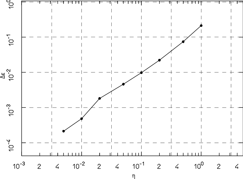
4.2 Numerical determination of the forcing frequency
In order to perform explicitly the algorithm constructing the Kolmogorov’s normal form (as described in the next section) for dissipative systems, we need to preliminarly determine the external forcing frequency. To fix the ideas, we limit ourselves to consider again the dynamics of the dissipative forced pendulum. The aim of this subsection is to determine, for a fixed invariant torus, the corresponding value of the parameter (appearing in the equation (6), where the Hamiltonian part is given in (4)). As discussed above, the frequency map provides the frequency of the quasi-periodic motion on an invariant torus as a function of the parameter . Now, the problem is the following: we fix the frequency related to an invariant torus and we need to approximate numerically the corresponding forcing frequency . Thus, denoting again the frequency map by , we want to find numerically the solution of the equation
This requires to invert the frequency map, or, more simply, to find the real zero of the function
For this purpose, we implement explicitly a Newton’s method which, as it is well known, is an iterative method to find numerically the solutions for this kind of problems. Let us stress that we expect to find a locally unique solution of the equation , because we obviously apply Newton’s method for values of the parameter smaller than the breakdown threshold of the invariant torus related to the frequency . Therefore, in a neighborhood of the unknown value , the function has a quasi-linear behavior, which looks strictly monotone, except in the resonant zones (see the left plots in Figure 2–3 and the discussions about them). Thus, if the initial approximation belongs to the region about the solution where the map looks mostly quasi-linear and monotone, Newton’s method is expected to be very efficient.
In order to be more definite, in the following we describe our procedure in detail. We denote with , the -th approximation of the solution ; then, the single step of Newton’s algorithm, applied to prescribes that the next approximation is given by
| (17) |
where the derivative is replaced by the finite difference and is a small parameter to be conveniently fixed so to ensure the numerical stability of this procedure. Of course, in formula (17) the values of and are numerically calculated, by using the frequency analysis. We stop the iterations when the relative correction on the value of is below a fixed precision , i.e., when
| (18) |
where is a small parameter that can be conveniently chosen so to be not much greater than the machine precision (let us recall that this is about for the standard double precision type numbers).
Let us remark that it is very unlikely that at some step the finite difference be close to , because it occurs that both and are in the same resonant region. In fact, the sizes of the resonant “plateaus” are smaller and smaller, when approaching the invariant torus; this fact can be seen in the left plots of Figures 2–3 and it has been clearly shown in the conservative framework (see, e.g., the numerical investigations in [47]). Thus, we limited ourselves to include a test in our code, to stop the running if the finite difference above is too small. This event is so rare that it never happened in our calculations; from a practical point of view, in such a case of failure, one has to look for a better initial approximation before restarting the procedure.
For instance, let us discuss an explicit case. We want to determine the value of the external forcing frequency such that the equations of motion (6) has the golden torus as an invariant attractor, when the values of the parameters are fixed so that
Let us recall that the value of the small parameter is chosen smaller than the breakdown threshold related to and (see the corresponding value of in the table appearing in Figure 4). We fix and and we start the Newton’s algorithm taking as initial approximation. In this case, the algorithm ends successfully after just steps with
| (19) |
As an internal test of our result, we performed the decomposition of the Fourier spectrum as in formula (10). Actually, we considered the motion on the invariant attractor for the dissipative forced pendulum defined by equation (6), with , and , with the value of given in (19). Since the golden torus is expected to be the invariant attractor, we tried to express every frequency as a linear combination of the components of the vector . The relevant quantities involved in the decomposition of the Fourier spectrum are listed in Table 6.2 of [62], where the numerical results definitely show that the invariant attractor is the golden torus related to the frequency .
5 Semi-analytic approach constructing the normal form for invariant tori
In order to describe the procedure constructing explicitly the Kolmogorov’s normal form related to an invariant quasi-periodic attractor, it is convenient to reformulate the pseudo-Hamiltonian model of the dissipative forced pendulum (defined by the equations (4)–(6)) in a suitably more general context. For this purpose, let us introduce three non-negative integer numbers , and ; among them, both and are strictly positive. Let be the number of degrees of freedom of the system described by the following equations of motion:
| (20) |
where is the external forcing frequency vector and the Hamiltonian part
| (21) |
In the equation above, as usual, must be regarded as a fixed frequency vector, while and , where we denote the class of functions which are homogeneous polynomials of degree in , , , do not depend on the actions , , and are trigonometric polynomials of degree with respect to the angles . Let us remark that also the Hamiltonian of the forced pendulum defined in (4) can be expressed in the form (21) with the following values of the integer parameters: , and . In fact, after having performed a translation33 3 Let us recall that is a canonical transformation. Moreover, we emphasize that in this special case the definition of here is given by avoiding the introduction of a new symbol instead of , by abuse of notation. of the action coordinate so that , it is enough to put , , , and .
Our goal is to determine an accurate approximation of a canonical transformation , such that in the new coordinates the equations of motion (20) are transformed to the following form:
| (22) |
where the new Hamiltonian is in Kolmogorov’s normal form, i.e.,
| (23) |
with . In words, the Kolmogorov’s normal form is such that its part depending on the angles is at least quadratic with respect to the actions. Therefore, the invariance of the torus immediately follows from the equations (22)–(23). Of course, that invariant torus is densely filled by a quasi-periodic orbit characterized by the frequencies vector .
5.1 Adapting the standard Kolmogorov’s normalization formal algorithm to dissipative equations with friction terms that are linear and homogeneous with respect to the actions
Let us describe the generic –th step of the adapted Kolmogorov’s normalization algorithm. We start from equations of motion of type
| (24) |
where the Hamiltonian part can be expanded as follows:
| (25) |
with and . Moreover, we require that the Taylor–Fourier series above is “well ordered”. This assumption is not restrictive, actually we mean that, and , each term appearing in the expansion of is such that and , where we used the common multi-index notation and is the –norm, for instance, .
The –th normalization step is split in two separate steps. We first remove part of the unwanted terms via a canonical transformation having as generating function. Lemma 2.4 of [63] ensures us that, after performing such a first canonical transformation, the new equations of motion have the following form:
| (26) |
where
| (27) |
and the new Hamiltonian part is given by
| (28) |
In order to avoid the proliferation of too many symbols, starting from equation (26) we do not introduce another set of variables for the new coordinates introduced after each canonical transformation; this is done by abuse of notation. Moreover, in the functional equation (28) the Lie series operator appears, where and is the classical Poisson bracket, a generic function defined on the phase space and any generating function.
Since we point to a Hamiltonian part of type (23), first, we determine the generating function so to remove both the main perturbing terms of degree and those that are linear with respect to the actions but do not depend on the angles. Thus, we solve with respect to and the equations
| (29) |
where the matrix is such that (let us recall that both and do not depend on the angles, because and ). After having expanded in Fourier series as
we can easily write the solution of the first homological equation appearing in (29), i.e.,
| (30) |
Let us emphasize that the solution above is well defined when the friction coefficient ; in the conservative case (i.e., ), it is enough to use the non-resonance condition (41), that will be explicitly adopted to solve the second homological equation. Moreover, one can easily realize that the second equation in (29), defines a linear system in the unknowns , because and ; this linear system can always be solved, provided that
| (31) |
Of course, the definition of is completed by setting .
We must now provide the expressions of the functions appearing in the expansion of the new Hamiltonian part
| (32) |
where is defined by the functional equation (28). To this aim, we will redefine many times the same quantity without changing the symbol. In our opinion, such a repeated abuse of notation has two advantages: first, this makes easier to understand the final calculation of instead of using one single very complicated formula; second, the description of the algorithm is more similar to its translation in a programming code. For instance, mimicking the C language, with the notation we mean that the previously defined quantity is redefined as . Therefore, we initially define
| (33) |
To take into account the Poisson bracket of the generating function with and the contribution of the term , we put
| (34) |
Then, we consider the contribution of the terms generated by the Lie series applied to each function as follows:
| (35) |
Looking at formulæ (33)–(35), one can easily check that and . We perform now a “reordering of the terms”, by moving the monomials in the expansions of to each others, in such a way that, at the end, each term of type belonging to the Taylor–Fourier (finite) series of the so redefined functions has degree in the actions and a trigonometric degree ; thus, it still holds true that .
In the second half of the –th step of the adapted Kolmogorov’s normalization algorithm, by using another canonical transformation, we remove the part of the perturbation up to the order of magnitude that actually depends on the angles and it is linear in the actions. For this purpose, we are going to determine a generating function that is linear with respect to the actions; therefore, lemma 2.3 of [63] ensures us that, after performing the canonical transformation related to , the new equations of motion have the following form:
| (36) |
where
| (37) |
and the new Hamiltonian part is given by
| (38) |
In order to approach a Hamiltonian part of type (23), it is convenient to solve the following equation with respect to :
| (39) |
After having expanded in Fourier series so that
| (40) |
if the following non-resonance condition is satisfied:
| (41) |
then we can easily write the solution of the second homological equation (39), i.e.,
| (42) |
Similarly to what we have done previously, we now provide the expressions of the functions appearing in the expansion of the new Hamiltonian part:
| (43) |
where is defined in (38). We initially define
| (44) |
The terms due to the expression do not depend on the actions and they contribute to the new Hamiltonian part as follows:
| (45) |
In view of the terms generated by the Lie series applied to and the second homological equation (39), we put
| (46) |
Moreover, the contribution of the Lie series applied to the rest of the Hamiltonian implies that
| (47) |
Finally, we perform a new “reordering of the terms”, so that at the end the functions (appearing in expansion (43)) contain just monomials of type with degree in the actions and trigonometric degree .
Let us recall that the canonical transformation inducing the Kolmogorov’s normalization up to the step is explicitly given by
| (48) |
This conclude the –th step of the algorithm that can be further iterated. Let us stress that the next step can be completely carried out, if both the non-degeneracy condition (31) and the non-resonant inequality (41) still hold true, when the index is replaced with . Actually, for what concerns the former assumption, this is usually ensured by requiring that both the quadratic part of the initial Hamiltonian is non-degenereate (i.e., ) and the parameter is small enough. Moreover, the latter non-resonance condition is usually satisfied for all indexes , provided the chosen frequency vector is Diophantine.
Let us emphasize that terms having different orders of magnitude with respect to the small parameter are not handled separately in our expansions. In particular, we prescribed to perform operations like the “reordering of the terms”, which explicitly requires to sum contributions corresponding to the same polynomial degree and Fourier harmonic, but with different orders in . The main advantage of this formulation is to save most of the memory occupation, when the algorithm is translated in any programming language (see the discussion at the end of section 4.1 of [29]). As a consequence of this gain in memory handling, more normalization steps can be performed (and in a faster way); let us stress that this can definitely improve the final accuracy of the results. From a practical point of view, when is expressed in the initial form (21), the parameter must be replaced by its numerical value. Therefore, in all the expansions written in the present subsection (whenever they are converging in some suitable domains), the sup-norm of the functions of type and is geometrically decreasing with respect to both the polynomial degree and the index , that is related to the their trigonometric degree .
5.2 Semi-analytic results
5.2.1 Checking the explicit construction of the Kolmogorov’s normal form
It could be astonishing that both the equations of motion (36) and the Hamiltonian part (43) defined at the -th normalization step have exactly the same structure as those introduced by the previous step, which are written in (24) and (25), respectively. Indeed, performing the algorithm described in the previous subsection is advantageous, because the unwanted Hamiltonian terms of degree and in the actions get smaller and smaller as increases (under the usual KAM hypotheses). This implies that the algorithm is successful if and only if also the generating functions decrease with (recall the equations (29) and (39)); this remark can be easily translated in a numerical test concerning the construction of the normal form.
The behavior of the sequence of the external forcing frequency vectors deserves a particular discussion. Let us recall that the main theorem in [63] actually proves the existence of a pair of objects: an initial frequency vector and a canonical transformation such that the equations of motion (20) are conjugated to those in (22), where the Hamiltonian part is in the Kolmogorov’s normal form (23). Thus, the proof scheme determines a posteriori, i.e., as a result of the normalization procedure (actually, here we followed the approach originally designed in [18]). Of course, this is unpractical when we focus on comparisons with numerical results, because any integrator of the equations of motion (20) requires that must be known in advance. This is the main reason why, in subsection 4.2 we developed a Newton method based on the frequency analysis, so to provide a good approximation of the initial , corresponding to the fixed angular velocity vector of the quasi-periodic motion on the wanted invariant torus. If such a vector would be perfectly determined, then the algorithm constructing the conjugacy to (22) (where any external frequency is not appearing) requires that for . In the following, we will test numerically this condition.

From a practical point of view, let us proceed to a further study of the equations of motion (6), where the Hamiltonian part is given in (4) and the values of the parameters are fixed so that
| (49) |
Let us recall that for this system the frequency analysis results of subsection 4.2 clearly show the existence of an attracting invariant torus, characterized by a quasi-periodic motion related to the golden frequency . In our opinion, the explicit construction of the normal form related to that torus is rather challenging, because the the perturbing parameter is larger than the breakdown threshold value for the conservative case (i.e., ) and at the same time it is not so far from the breakdown threshold corresponding to the chosen friction coefficient (i.e., , see the table appearing in Figure 4).
Of course, it is convenient to reformulate the equations of motion in the form where all the terms appearing in the expansion of the Hamiltonian are determined as in the discussion following formula (21). In particular, we have
Starting from these settings, we explicitly performed steps of the normalization procedure described in subsection 5.1, by using the software package Xó, that is designed for making computer algebra, with a special care to its possible applications to Celestial Mechanics problems (see [32] for an introduction to its main concepts). Since none of the canonical transformations prescribed by the algorithm increases the polynomial degree, all the expansions of the Hamiltonian parts are rather compact, because they are at most quadratic in the actions as the initial . Figure 5 shows the norms of the generating functions , and with the index ; more precisely, we have calculated the sum of the absolute values of the coefficients appearing in (30), (29) and (42), respectively. Actually, the precision of the computation is affected by the truncation rules on the expansions, that we arranged so to neglect all the terms having a Fourier harmonic with –norm . In particular, this implies also that the contributions due to many relevant terms independent from the angles are not taken into account for ; thus, the plot of has been stopped when the values corresponding to some indexes have begun to be unrealistically small with respect to the previous ones. Let us emphasize that the geometrical decrease of the generating functions looks quite sharp in the semi–log scale of Figure 5; this behavior is in agreement with the analytical estimates on the algorithm constructing the Kolmogorov’s normal form, when it is reformulated according a classical formal scheme (see [30]). Furthermore, also the –norm of the external forcing frequency vector is reported in Figure 5. In this case, the geometrical decrease is rather sharp until a “saturation threshold value”, that is of order ; for the value of is approximately constant. This unpleasant phenomenon can be easily explained, by taking into account that the numerical determination of the initial is affected by the unavoidable round-off errors. Such an uncertainity (due to the application of the frequency analysis numerical method) is propagated to all the sequence of the external forcing frequency vectors by the recursive definitions (27) and (37). Thus, the computed plot of agrees with the expectation that . Finally, we can conclude that Figure 5 makes evident that the constructing procedure is converging to the Kolmogorov’s normal form for dissipative systems, which is characterized by equations (22) and (23).
We now perform another test, checking the accuracy of the conjugacy canonical transformation which is provided after having carried out the –th normalization step according to the definition (48). Some previous works studying the construction of the Kolmogorov’s normal form stressed that it can be used to integrate the equations of motion on an invariant torus characterized by a frequency vector . In fact, one can refer to the following ideal scheme (see, e.g., [49] and [29]):
| (50) |
where is nothing but the flow induced by , that is the only effective part for the normalized equations of motion (22)–(23), when ; moreover, let us recall that is the conjugacy transformation whose existence is ensured by a KAM–like statement (under suitable hypotheses). Of course, cannot be explicitly calculated, but this can be done for (a truncated expansion of) with a possibly large value of the index . Thus, it is convenient to limit ourselves to consider a numerical approximation of the motion law on an invariant torus characterized by a frequency vector , so to check if the following relation is satisfied:
| (51) |
where provides the approximately normalized –th action for .

We check formula (51) with and, again, in the special case of the dissipative forced pendulum, that is defined by the equations (6) and (4) with the values of the parameters given in (49). In particular, we consider the motion law on the attracting invariant torus, related to the golden frequency . In Figure 6a, we report the values of the approximately normalized action as a function of its canonically conjugated angle , when . Let us stress that the initial value of (and the corresponding ) is unrelevant, when we are interested in checking the accuracy of the normalized canonical coordinates on all the invariant torus, because it is filled by the quasi-periodic orbit. However, the pair is determined after having integrated the equations of motion for a relaxation time-span, according to the discussion reported at the end of section 2. Let us also remark that it is natural to neglect completely the second pair of coordinates; in fact, we recall that the dummy action does not affect the evolution of all other canonical variables; moreover, since , the second angle just describes the flowing of time. For this reason we have chosen to plot the approximately normalized first action when , as in a standard Poincaré map. Figure 6a highlights that the action (making part of the nearly normalized set of canonical variables) is close to zero for all the considered points generated by the Poincaré map of the flow on the attracting golden torus, in agreement with (51). Actually, the maximum of is a few orders of magnitude bigger than the round-off errors threshold, as expected because their accumulation is unavoidable, while the very large number of computations required by the expansions are explicitly performed.
We now check the behavior of formula (51) as a function of the final normalization step . Since the ideal normalization transformation is such that , then we expect that
| (52) |
where denotes again the motion law on the attracting golden torus. The results of our tests of the previous formula are illustrated in Figure 6b, where the appearing in the r.h.s. is approximated with the maximum on the index ranging in . Also in this case, the plot nicely shows a geometrically decreasing behavior, in agreement with the expectations (see [30]). This positively ends the check of the explicit construction of the conjugacy canonical transformation.
5.2.2 The basin of attraction of an invariant torus: a semi-analytic lower estimate
Let us now focus on the dynamics in a region surrounding an invariant torus, as it is described by normalized coordinates. This means that we are going to study the equations of motion (22), where the Hamiltonian is of type (23), that is in Kolmogorov’s normal form. Moreover, let us suppose to know some upper bounds on the size of its terms which depend on the angles and, then, are at least quadratic with respect to the actions. This allows us to easily produce some estimates on the basin of attraction, by adapting a standard technique commonly used in the local theory around an equilibrium point of ordinary differential equations.
For the sake of simplicity, we summarize the argument by referring to the Kolmogorov’s normal form of the specific case of a dissipative forced pendulum, where the pseudo-Hamiltonian equations of motion are the following:
| (53) |
where and is the frequency vector characterizing the quasi-periodic motion on the invariant torus . It is convenient to study the integral form of the first component of the differential equations system (53), that is
| (54) |
Since we supposed to be able to evaluate the size of the terms depending on the angles, we can assume to know such that
| (55) |
Therefore, the following inequality can be immediately deduced starting from (54):
| (56) |
Let us consider a generic initial condition belonging to a (not arbitrarily large) set such that and
| (57) |
with . Let us define the positive44 4 Let us remind that, by using (55), the velocity can be easily bounded on the compact set ; thus, cannot be equal to . time so that
| (58) |
where is nothing but the motion law of the coordinate starting from the initial conditions . Here, it is convenient to introduce . Starting from (56), we can write the following chain of inequalities:
| (59) |
where we used the well known Gronwall’s lemma. The previous formula can be rephrased for the law motion of the variable , so that . Therefore, also and then we can extend the procedure also to the time intervals , and so on. This allows us to justify the exponential estimate . Since the parameter can be made arbitrarily small, we can finally conclude that
| (60) |
Let us emphasize that this same approach can be rather trivially extended, so to obtain the same result for higher dimensions pseudo-Hamiltonian equations of motion, where the initial Kolmogorov’s normal form Hamiltonian is of type (23).
Formula (60) can be directly applied to the dissipative forced pendulum, so to locate a subset of the basin of attraction of the invariant torus. In fact, let us consider an initial condition
| (61) |
where is the change of coordinates55 5 Actually, here we avoid to consider the effect of the change of coordinates on the dummy actions and , because they do not affect the evolution of all other variables. In the present subsection, this abuse of notation will be made also for the transformation approximating . appearing in the ideal scheme (50); this means that it brings the pseudo-Hamiltonian equation of motion to the Kolmogorov’s normal form. Therefore, the corresponding motion law tends (in an exponentially fast way) to the invariant tous, in view of (60) and because is canonical (see [63]). For practical purposes, the change of coordinates must be replaced, of course, by , that is defined in (48) and is given by the composition of the transformations related to the first normalization steps. Figure 7 represents the intersection of the initial conditions (61) with the plane ; they are located in the region between the two dashed curves. Actually, those curves have been drawn by plotting the inverse image of the two rings with respect to the map , in the case of the dissipative forced pendulum equations (4)–(6), when the values of the parameters are fixed so that
In that case, there are two attractors: the invariant torus corresponding to the vector frequency and a periodic orbit; their corresponding sections with the plane are located by a solid line, that can be seen in Figure 7, and a fixed point having coordinates , respectively. By the way, let us recall that other examples of dissipative systems showing the coexistence of more than one attractor are described in [17]. The change of coordinates , that is a good approximation of the ideal normalizing transformation , is calculated by following the detailed discussion of subsections 5.1 and 5.2.1; moreover, is evaluated so to satisfy inequality (55), when the remainder is replaced by the finite sum of the quadratic terms belonging to the calculated truncation of the Hamiltonian . Of course, the drawing of the section of the initial conditions (61) is made in a numerical way; nevertheless, we emphasize that the procedure could be made completely rigorous, so to determine a set that is certainly included in the basin of attraction of the invariant torus, by implementing interval arithmetics and providing analytic estimates of all the truncated terms (see, e.g., [22]). The effects of such a computer-assisted procedure are expected to be completely unrelevant in a plot like that of Figure 7. In order to check the effectiveness of our procedure, the basin of attraction of the periodic orbit is drawn in black in Figure 7. Of course, the area provided by our estimates cannot cover a rather significant part of the basin of attraction of the invariant torus, that is actually expected to be infinitely big, because it is the complementary of the black region appearing in Figures 7a and 7b. Nevertheless, we think that our approach can be useful to develop computational methods also in dissipative systems with a larger number of degree of freedom. Indeed, it could help to locate an initial thin region of the basin of attraction surrounding the possibly complicated shape of an invariant torus; therefore, the computational strategy could include suitable numerical integrations backwards in time, so to reconstruct all the parts of the phase space that are potentially belonging to the basin; moreover, some final forward integrations (taking care of the propagation of the errors) could validate the location of most of the basin of attraction.

6 Conclusions
Since the sixities and during a couple of decades, KAM theorem was commonly considered to be a very elegant mathematical result, but substantially irrelevant for real problems in physics, because the hypothesis on the smallness of the perturbation was (and still is) extremely restrictive (see [38]). Indeed, several articles appeared since the eighties actually showed that KAM theory can be effectively applied to realistic models, provided that it is complemented with suitable computational techniques (see, e.g., [16]). In our opinion, this work adds a few new arguments to such a more modern point of view.
KAM theory provides the natural framework to define the frequency analysis method, which discriminates between quasi-periodic motions and chaotic ones in Hamiltonian systems ([43] and [44]); this allows a global understanding of the dynamics. In section 3, that computational approach has been adapted to a special class of dissipative systems with friction terms, that are linear and homogeneous with respect to the actions. The method is based on a clear interpretation of the results, that can be nicely visualized. Moreover, our evaluation of the breakdown threshold for invariant tori in the dissipative standard map is in agreement with some existing results in literature (see [8]). Actually, our method is less precise than that based on the computation of the Sobolev norms, also because our approach, which is extremely visual, is hard to made automatic; this strongly limits the performances when a great accuracy is required. This is also the reason why, in our opinion, the numerical results given in section 4 (about the breakdown threshold of invariant tori for the dissipative forced pendulum) show just partially the expected behavior.
In section 5, the explicit algorithm constructing the Kolmogorov’s normal form has been adapted so to cover also the case of dissipative systems having a pseudo-Hamiltonian framework. Moreover, such a reformulation has been successfully applied to the dissipative forced pendulum model: by a code implementing algebraic manipulations on a computer, the shape of an attracting invariant “golden” torus (related to some specific values of the parameters) has been carefully reconstructed. We emphasize that such a result was expected, but it is not trivial, because the constructive algorithm producing the normal form for the dissipative case is significantly different with respect to that traditionally used in KAM theory for Hamiltonian systems. Let us recall that the good system of equations (for which the “golden” torus is invariant and attracting) has been settled by using the frequency analysis, so to determine a priori the numerical value of one of the parameters (namely, the external frequency in (49)). In our opinion, this fact validates our implementations of both the frequency analysis and the construction of the Kolmogorov’s normal form, because two so different techniques provide results that are in agreement between them. As a further natural application of a method based on a normal form, in the last subsection 5.2.2, the contracting dynamics in a neighborhood of an invariant torus is estimated by using the Gronwall’s inequality. This has allowed us to show that such an open set is certainly included in the basin of attraction of that invariant torus.
Acknowledgments
A. Celletti encouraged us to study the particular class of dissipative systems considered in the present paper. A. Giorgilli allowed us to use the computer algebra package Xó, initially written by himself with the late (and relevant) contribution of M. Sansottera. A. Noullez suggested us how to improve our numerical code doing frequency map analysis. We are deeply indebted with all of them.
References
- [1] Abad, A., Barrio, R., Blesa, F., Rodriguez, M.: Algorithm 924: TIDES, a Taylor Series Integrator for Differential EquationS, ACM Transactions on Math. Software, 39, Issue 1, Article No.: 5 (2012).
- [2] Arnold V.I.: Proof of a theorem of A. N. Kolmogorov on the invariance of quasi-periodic motions under small perturbations of the Hamiltonian, Usp. Mat. Nauk, 18, 13 (1963); Russ. Math. Surv., 18, 9 (1963).
- [3] Bambusi, D., Haus, E.: Asymptotic stability of synchronous orbits for a gravitating viscoelastic sphere, Cel. Mech. & Dyn. Astr., 114, 255–277 (2012).
- [4] Benettin, G., Galgani, L., Giorgilli, A., Strelcyn, J.M.: A Proof of Kolmogorov’s Theorem on Invariant Tori Using Canonical Transformations Defined by the Lie method, Nuovo Cimento, 79, 201–223 (1984).
- [5] Biasco, L., Chierchia, L.: Low-order resonances in weakly dissipative spin-orbit models, J. Diff. Equations, 246, 4345–4370 (2009).
- [6] Broer, H.W., Huitema, G.B., Sevryuk, M.B.: Quasi-periodic Motions in Families of Dynamical Systems. Order Amidst Chaos, Lecture Notes in Mathematics, 1645, Springer–Verlag, Berlin (1996).
- [7] Broer, H.W., Simò, C., Tatjer, J.C.: Towards global models near homoclinic tangencies of dissipative diffeomorphisms, Nonlinearity, 11, 667–770 (1998).
- [8] Calleja, R., Celletti, A.: Breakdown of invariant attractors for the dissipative standard map, CHAOS 20, issue 1, 013121 (2010).
- [9] Calleja, R., Celletti, A., de la Llave, R.: A KAM theory for conformally symplectic systems: Efficient algorithms and their validation, J. Diff. Equations, 255, 978–1049 (2013).
- [10] Calleja, R., Celletti, A., de la Llave, R.: Local behavior near quasi-periodic solutions of conformally symplectic systems, J. Dyn. & Diff. Equations, 25, 821-841 (2013).
- [11] Calleja, R., de la Llave, R.: A numerically accessible criterion for the breakdown of quasi-periodic solutions and its rigorous justification, Nonlinearity, 23, 2029–2058 (2010).
- [12] Celletti, A.: Analysis of resonances in the spin–orbit problem in Celestial Mechanics: the synchronous resonance (Part I)., J. of App. Math. and Phys. (ZAMP), 41, 174 (1990).
- [13] Celletti, A.: Analysis of resonances in the spin–orbit problem in Celestial Mechanics: higher order resonances and some numerical experiments (Part II)., J. of App. Math. and Phys. (ZAMP), 41, 453 (1990).
- [14] Celletti, A.: Periodic and Quasi-Periodic Attractors of Weakly-dissipative Nearly-integrable Systems, Reg. & Ch. Dyn., 14, 49–63 (2009).
- [15] Celletti, A., Stability and Chaos in Celestial Mechanics, Springer-Praxis (2010).
- [16] Celletti, A., Chierchia, L.: KAM Stability and Celestial Mechanics, Memoirs American Mathematical Society, 187 (2007).
- [17] Celletti, A., Chierchia, L.: Measures of basins of attraction in spin-orbit dynamics, Cel. Mech. & Dyn. Astr., 101, 159–170 (2008).
- [18] Celletti, A., Chierchia, L.: Quasi-Periodic Attractors in Celestial Mechanics, Arch. Rat. Mech. Anal., 191, 311–345 (2009).
- [19] Celletti, A., Di Ruzza, S.: Periodic and quasi-periodic orbits of the dissipative standard map, DCDS-B, 16, 151–171 (2011).
- [20] Celletti, A., Di Ruzza, S., Lhotka, C., Stefanelli, L.: Nearly-Integrable Dissipative Systems and Celestial Mechanics, The European Phys. Jour. - Special Topics, 186, no. 1, 33–66 (2010).
- [21] Celletti, A., Froeschlé, C, Lega, E.: Dissipative and weakly-dissipative regimes in nearly-integrable mappings, DCDS-A, 16, no. 4, 757–781 (2006).
- [22] Celletti, A., Giorgilli, A., Locatelli, U.: Improved Estimates on the Existence of Invariant Tori for Hamiltonian Systems, Nonlinearity, 13, 397–412 (2000).
- [23] Chandre, C., Laskar, J., Benfatto, G., Jauslin, H.R.: Determination of the breakup of invariant tori in three frequency Hamiltonian systems, Physica D, 154, 159–170 (2001).
- [24] Chierchia, L.: A. N. Kolmogorov’s 1954 paper on nearly-integrable Hamiltonian systems, Reg. & Ch. Dyn., 13, 130–139 (2008).
- [25] Correia, A.C.M., Laskar, J.: Mercury’s capture into the 3/2 spin-orbit resonance as a result of its chaotic dynamics, Nature, 429, 848–850 (2004).
- [26] Deprit, A., Deprit–Bartholomé, A.: Stability of the Triangular Lagrangian Points, Astron. J., 72, 173 (1967).
- [27] D’Hoedt, S., Lemaître, A.: Planetary long periodic terms in Mercury’s rotation: a two dimensional adiabatic approach, Cel. Mech. & Dyn. Astr., 101, 127–139 (2008).
- [28] Dumas, S., Laskar, J.: Global Dynamics and Long-Time Stability in Hamiltonian Systems via Numerical Frequency Analysis, Phys. Rev. Lett., 70, 2975–2979 (1993).
- [29] Gabern, F., Jorba, A., Locatelli, U.: On the construction of the Kolmogorov normal form for the Trojan asteroids, Nonlinearity, 18, n.4, 1705–1734 (2005).
- [30] Giorgilli, A., Locatelli, U.: Kolmogorov theorem and classical perturbation theory, J. of App. Math. and Phys. (ZAMP), 48, 220–261 (1997).
- [31] Giorgilli, A., Locatelli, U., Sansottera, M.: Kolmogorov and Nekhoroshev theory for the problem of three bodies, Cel. Mech. & Dyn. Astr., 104, 159–173 (2009).
- [32] Giorgilli, A., Sansottera, M.: Methods of algebraic manipulation in perturbation theory, in P.M. Cincotta, C.M. Giordano and C. Efthymiopoulos (eds.): “Chaos, Diffusion and Non-integrability in Hamiltonian Systems - Applications to Astronomy, Proceedings of the 3rd La Plata International School on Astronomy and Geophysics”, Universidad Nacional de La Plata and Asociación Argentina de Astronomía Publishers, La Plata (2012).
- [33] Goldreich, P., Peale, S.J.: Spin-orbit coupling in the Solar System, Astron. J., 71, 425–438 (1966).
- [34] Goldreich, P., Peale, S.J.: The dynamics of planetary rotations, Ann. Rev. Astron. Astrophys., 6, 287–320 (1970).
- [35] Govin, M., Chandre, C., Jauslin, H. R.: KAM–Renormalization–Group analysis of stability in Hamiltonian flows, Phys. Rev. Lett., 79, 20, 3881–3884 (1997).
- [36] Greene, J.M., A method for determining a stochastic transition, J. of Math. Phys 20, 1183–1201 (1979).
- [37] Haus, E., Bambusi, D.: Asymptotic behavior of an elastic satellite with internal friction, available at webpage http://arxiv.org/abs/1212.0816, preprint (2012).
- [38] Henon, M.: Exploration numérique du problème restreint IV: Masses égales, orbites non périodiques, Bulletin Astronomique, 3, N. 1, fasc. 2, 49–66, (1966).
- [39] Gomez, G., Mondelo, J.M., Simò, C.: A collocation method for the numerical Fourier analysis of quasi-periodic functions. I: Numerical tests and examples, DCDS-B, 14, 41–74 (2010).
- [40] Gomez, G., Mondelo, J.M., Simò, C.: A collocation method for the numerical Fourier analysis of quasi-periodic functions. II: Analytical error estimates, DCDS-B, 14, 75–109 (2010).
- [41] Jorba, A., Zou, M.: A Software Package for the Numerical Integration of ODEs by Means of High-Order Taylor Methods, Experiment. Math., 14, 99–117 (2005).
- [42] Kolmogorov, A.N.: Preservation of conditionally periodic movements with small change in the Hamilton function, Dokl. Akad. Nauk SSSR, 98, 527 (1954). Engl. transl. in: Los Alamos Scientific Laboratory translation LA-TR-71-67; reprinted in: Lecture Notes in Physics 93.
- [43] Laskar, J.: Introduction to frequency map analysis, in C. Simò (managing ed.), Proceedings of the NATO ASI school: “Hamiltonian Systems with Three or More Degrees of Freedom”, S’Agaro (Spain), June 19–30, 1995, Kluwer, 134–150 (1999).
- [44] Laskar, J.: Frequency Map analysis and quasi periodic decompositions, in Benest et al. (managing eds.): “Hamiltonian systems and Fourier analysis”, Taylor and Francis (2005).
- [45] Laskar, J., Froeschlé, C., Celletti, A.: The measure of chaos by the numerical analysis of the fundamental frequencies. Application to the standard mapping, Physica D 56, 253–269 (1992).
- [46] Laskar, J., Robutel, P.: The chaotic obliquity of the planets, Nature, 361, 608–612 (1993).
- [47] Lega, E., Froeschlé, C.: Numerical investigations of the structure around an invariant KAM torus using the frequency map analysis, Physica D, 95, 97–106 (1996).
- [48] Leontovich, A. M.: On the stability of the Lagrange periodic solutions for the reduced problem of three bodies, Soviet Math. Dokl., 3, 425 (1962).
- [49] Locatelli, U., Giorgilli, A.: Invariant tori in the secular motions of the three–body planetary systems, Cel. Mech. & Dyn. Astr., 78, 47–74 (2000).
- [50] Locatelli, U., Giorgilli, A.: Construction of the Kolmogorov’s normal form for a planetary system, Reg. & Ch. Dyn., 10, 153–171 (2005).
- [51] Locatelli, U., Giorgilli, A.: Invariant tori in the Sun–Jupiter–Saturn system, DCDS-B, 7, 377–398 (2007).
- [52] MacDonald, G.J.F.: Tidal friction, Rev. Geophys., 2, 467–541 (1964).
- [53] MacKay, R. S.: Greene’s residue criterion, Nonlinearity, 5, 161–187, (1992).
- [54] Morbidelli, A., Giorgilli, A.: Superexponential stability of KAM tori, J. Stat. Phys., 78, 1607–1617 (1995).
- [55] Moser, J.: On invariant curves of area–preserving mappings of an annulus, Nachr. Akad. Wiss. Gött,. II Math. Phys. Kl 1962, 1–20 (1962).
- [56] Noullez, A.: Chaos characterization in Hamiltonian systems using resonance analysis, in Dynamics of Celestial Bodies DCB-08 International Conference Proceedings, 147–150 (2009).
- [57] Papaphilippou, Y., Laskar, J.: Global dynamics of triaxial galactic models through frequency map analysis, Astron. & Astrophys., 329, 451–481 (1998).
- [58] Peale, S.J.: The free precession and libration of Mercury, Icarus, 178, 4–18 (2005).
- [59] Pöschel, J.: Integrability of Hamiltonian systems on Cantor sets, Comm. Pure Appl. Math., 35, 653–695 (1982).
- [60] Robutel, P., Laskar, J.: Frequency Map and Global Dynamics in the Solar System I: Short Period Dynamics of Massless Particles, Icarus, 152, 4–28 (2001).
- [61] Sansottera, M., Locatelli, U., Giorgilli, A.: A semi-analytic algorithm for constructing lower dimensional elliptic tori in planetary systems, Cel. Mech. & Dyn. Astr., 111, 337–361 (2011).
- [62] Stefanelli, L.: Periodic and quasi-periodic motions in nearly-integrable dissipative systems with application to Celestial Mechanics, Ph.D. Thesis, Univ. Roma “Tor Vergata” (2011).
- [63] Stefanelli, L., Locatelli, U.: Kolmogorov’s normal form for equations of motion with dissipative effects, DCDS-B, 17, 2561–2593 (2012).