Detecting the work statistics through Ramsey-like interferometry

The assessment of out-of-equilibrium statistics of quantum systems subjected to time-dependent processes is attracting an increasing degree of attention from the community interested in modern quantum physics[1]. The Crooks and Jarzynski relations[2, 3, 4], which take into account fluctuations in non-equilibrium dynamics, connect thermodynamical properties at equilibrium to the non-equilibrium details of dynamics. The verification of their quantum mechanical counterparts has so far encountered substantial difficulties due to the practical difficulty to perform reliable projective measurements of instantaneous energy states[1, 5], which are steps required in order to fully reconstruct the statistics of work.

In Refs. \refciteDorner and \refciteMazzola, a radical change to the approach for the reconstruction of the work statistics has been proposed, inspired by phase-estimation protocols that are well-known in quantum information processing. The method, which relies on the use of a clean and controllable ancilla, suitably coupled to the system of interest, has very recently enabled the first experimental characterization of quantum fluctuation relations[8]. Together with more recent schemes designed to address the quantum scenario[5, 9, 10], this has embodied a significant complement to past experimental successful verifications of out-of-equilibrium fluctuation relations in classical systems[11, 12, 13, 14, 15].

In this paper we extend the discussion presented in Ref. \refciteMazzola by emphasising the versatility of the proposed interferometric approach to the reconstruction of the characteristic function and apply it to the study of the statistics of work done by an external driving potential that changes the frequency of a harmonic oscillator. This problem is key in the current theoretical design of Otto cycles based on trapped-ion technology[16], and this physical situation is indeed encountered in a number of experimental scenarios, from cavity-quantum electrodynamics to its superconducting-circuit counterpart.

The remainder of this paper is organised as followed. In Sec. 2 we give a brief review of the interferometric scheme at the core of our analysis. Sec. 3 illustrates its application to the physical situation depicted above. In Sec. 4 we extend our approach to the case of an additional auxiliary system, much in the spirit of the proposal put forward by Campisi et al. in Ref. \refciteCampisiNJP. Finally, Sec. 5 summarises our findings and discusses the remaining open questions in this tantalising area.

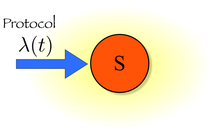
Let us consider the situation illustrated pictorially in Fig. 1 (a). A system $S$ with ‘bare’ Hamiltonian $\hat{\cal H}_{B}$, describing its free evolution, is affected by a protocol described by a Hamiltonian $\hat{\cal H}_{P}(\lambda_{t})$, which depends on an externally controlled work parameter $\lambda(t)\equiv\lambda_{t}$, so that the total Hamiltonian is $\hat{\cal H}_{S}(\lambda_{t})=\hat{\cal H}_{B}+\hat{\cal H}_{P}(\lambda_{t})$. We assume that at the initial time $t=0^{-}$ the system is in contact with a bath at inverse temperature $\beta$, so that $S$ is initialised in the thermal state

Here $\lambda_{0}$ is the initial value of the external parameter and $\mathcal{Z}(\lambda_{t})=\textrm{Tr}{e^{{-\beta\hat{\cal H}_{S}(\lambda_{t})}}}$ is the partition function. At $t=0^{+}$, $S$ is detached from the reservoir, while the protocol bringing $\lambda_{t}$ from $\lambda_{0}$ to its final value $\lambda_{\tau}$ starts. In order to define the probability distribution of work and its characteristic function, it is useful to write the Hamiltonian $\hat{\cal H}_{S}(\lambda_{t})$ at the initial and final time of the protocol in terms of the corresponding spectral decomposition. That is

where $E_{n}$ ($E^{\prime}_{M}$) is the $n^{\text{th}}$ ($M^{\text{th}}$) eigenvalue of the initial (final) Hamiltonian associated with the eigenvector $\left|n\right\rangle$ ($\left|M\right\rangle$). The corresponding work distribution can be written as [2]

Here $p(n,M)=\mathrm{Tr}[\left|M\right\rangle\left\langle M\right|\hat{U}_{\tau}\left|n\right\rangle\left\langle n\right|\rho_{S}\left|n\right\rangle\left\langle n\right|\hat{U}^{\dagger}_{\tau}]$ is the joint probability of finding the system in $\left|n\right\rangle$ at time $t=0$ and in state $\left|M\right\rangle$ at time $\tau$, after the evolution ruled by the time-propagator $\hat{U}_{\tau}$. Obviously, such a joint probability can be decomposed as $p(n,M)=p^{0}_{n}\;p^{\tau}_{M|n}$, where $p_{n}^{0}$ is the probability that the system is found in state $\left|n\right\rangle$ at time $t=0$ and $p^{\tau}_{M|n}$ is the conditional probability to find $S$ in $\left|M\right\rangle$ at time $\tau$ if it was initially in $\left|n\right\rangle$. Therefore, $P(W)$ bears information on the statistics of the initial state and the fluctuations arising from quantum dynamics and measurement statistics. The characteristic function of the work probability distribution of $P(W)$ is then defined as[19]

We shall now recall the interferometric scheme for the determination of $\chi(u)$ presented in Ref. \refciteMazzola. Let us introduce an ancillary qubit $A$ encoded in the energy states of a two-level system $\{\left|0\right\rangle_{A},\left|1\right\rangle_{A}\}$. We prepare the ancilla in $\left|0\right\rangle_{A}$ and apply a Hadamard transform $\hat{H}=(\hat{\sigma}_{x}+\hat{\sigma}_{z})/\sqrt{2}$ [21] that changes such state into $\left|+\right\rangle_{A}=(\left|0\right\rangle_{A}+\left|1\right\rangle_{A})/\sqrt{2}$. We then apply the system-ancilla evolution operator

to their joint state $\left|+\right\rangle\!\left\langle+\right|_{A}\otimes\rho^{th}_{S}$. In Eq. (5) we have introduced the notation $\hat{\cal H}_{S}^{i}=\hat{\cal H}_{S}(\lambda_{0})$ [$\hat{\cal H}_{S}^{f}=\hat{\cal H}_{S}(\lambda_{\tau})$]. We then subject $A$ to a second Hadamard transform and trace over the degree of freedom of the system. The ancilla is correspondingly found in a state that depends on $\chi(u)$ as

with $\alpha=\textrm{Re}\chi(u)$ and $\nu=\textrm{Im}\chi(u)$, and $\hat{\sigma}_{x,y,z}$ the Pauli operators of the ancillary qubit. From this analysis it should be clear that $\chi(u)$ can be easily reconstructed by measuring the longitudinal and transverse magnetization $\langle\hat{\sigma}_{z,A}\rangle$ and $\langle\hat{\sigma}_{y,A}\rangle$ for every value of $u$ deemed necessary. Notice that $\hat{G}(u)$ can be decomposed into local transformations and $A$-controlled gates as $\hat{G}(u)=(\hat{I}_{S}\otimes\hat{\sigma}_{x,A})\hat{G}_{2}(u)(\hat{I}_{S}\otimes\hat{\sigma}_{x,A})\hat{G}_{1}(u)$ with

Much in analogy with the inference of a relative phase originated by a dynamics in a phase-estimation protocol, our scheme clearly relies on the interference between orthogonal ‘evolution paths’ of the system, which are to interfere at the end of the scheme (thanks to the mixing operated by the second Hadamard gate) and are imprinted in the state of the ancilla. The scheme is reminiscent of a Ramsey-like interferometer[20], which thus motivates and justify our claim for an interferometric approach to the reconstruction of the work statistics following a process.

We emphasise that we did not make any assumptions on the form of $\hat{\cal H}_{S}(\lambda_{t})$. In fact we allow the Hamiltonian to not commute with itself (at different instant of time) and with the unitary evolution operator. That is, our approach can be equally adopted in the cases $[\hat{\cal H}^{i}_{S},\hat{\cal H}_{S}^{f}]\neq 0$ and $[\hat{U}_{\tau},\hat{\cal H}^{i(f)}_{S}]\neq 0$. However if such commutators are null, a much simpler version of the protocol holds, as the conditional gate in Eq. (5) simply becomes

The protocol proceeds exactly as described above with the the replacement $\hat{G}(u)\rightarrow\hat{G}^{S}(u)$. As shown above, $\hat{G}^{S}(u)$ can be split in two $A$-controlled gates and local transformation (as in the general case) as $\hat{G}^{S}(u)=(\hat{I}_{S}\otimes\hat{\sigma}_{x,A})\hat{G}^{S}_{2}(u)(\hat{I}_{S}\otimes\hat{\sigma}_{x,A})\hat{G}^{S}_{1}(u)$ with

We now discuss an explicit physical scenario in which our interferometric scheme can be applied and illustrated efficiently. In details, we consider a harmonic oscillator whose frequency, representing the work parameter $\lambda_{t}$ of the protocol, is changed in time according to a chosen functional form. The Hamiltonian of the system is thus

with $\lambda_{t}$ that is changed in time. For illustrative purposes, here we concentrate on the case of a sudden quench of the frequency of the oscillator[22], the case of a generic temporal dependence being only a generalisation of the forthcoming discussion. It is straightforward to check that, in this case, the characteristic function of the work distribution following the frequency quench is given by

where $\Delta\lambda=\lambda_{\tau}-\lambda_{0}$ and $\overline{n}$ is the mean number of excitations in the initial thermal state $\rho^{th}_{S}(0^{-})=\sum^{\infty}_{n=0}\frac{\overline{n}^{n}}{(1+\overline{n})^{n+1}}\left|n\right\rangle\left\langle n\right|$. This function depends crucially on the amplitude of the quench $\Delta\lambda$ and the mean thermal number $\overline{n}$. For no quench (i.e. $\Delta\lambda=0$), $\chi(u)=1$ and no work is done on the harmonic oscillator. On the other hand, there are values of the quench amplitude that correspond to the occurrence of ‘resonances’ in $\chi(u)$, as it is seen from Figs. 2 and 3. The consequences of such dependences are more clearly seen from the form taken by the corresponding $P(W)$ and the average work $\langle W\rangle$.

The first is determined by taking the anti-Fourier transform of $\chi(u)$, in line with the definition given in Eq. (4). In order to gather analytic insight into this problem, we have evaluated the integral

which is such that $P(W)=\lim_{\epsilon\to\infty}{\cal I}(\epsilon)$. We get

with $a=1/2-W/\Delta\lambda$, $z=e^{-i\epsilon\Delta\lambda}\overline{n}/(1+\overline{n})$, and ${}_{2}F_{1}(\alpha,\beta;\gamma,z)$ the Hypergeometric function. For $\overline{n}=0$, we have $z=0$ and ${}_{2}F_{1}(\alpha,\beta;\gamma,0)=1$. This implies that

Therefore, $\lim_{\epsilon\to\infty}{\cal I}(\epsilon)=\delta(W-\Delta\lambda/2)$, which is in line with the physical expectations at null temperature. For $\overline{n}\neq 0$, on the other hand, it is convenient to use the power-series definition of the Hypergeometric function, i.e. ${}_{2}F_{1}(\alpha,\beta;\gamma,z)=\sum^{\infty}_{n=0}\frac{(\alpha)_{n}(\beta)_{n}}{(\gamma)_{n}}\frac{z^{n}}{n!}$ with $(q)_{n}$ the Pochhammer symbol of argument $q$. For the specific case at hand, we have that

In turn, this implies that the probability distribution of work is made out of Dirac-delta peaks centred at $(n+1/2)\Delta\lambda$ and of amplitude $\overline{n}^{n}/(1+\overline{n})^{n+1}$, which are dictated by the statistics of the initial thermal state. Two instances of such distribution are illustrated in Fig. 4, where we see that higher temperatures correspond to the emergence of many peaks in $P(W)$ due to the large number of states entering $\rho^{th}_{S}(0^{-})$ and a correspondingly large number of state transitions.

As for the average work, this can be easily determined using the characteristic function $\chi(u)$ as $\langle W\rangle=-\left.i\partial_{u}\chi(u)\right|_{u=0}$, whose explicit evaluation gives us

showing that the average work linearly increases with the amplitude of the quench and the mean thermal number of excitations.

We now show that a suitable coupling between the system and an ancilla qubit allows us to generate the conditional operations, introduced in the previous Section, necessary for the interferometric reconstruction of the characteristic function. In order to fix the ideas, we can think of the harmonic oscillator as embodied by the fundamental flexural mode of a suspended double-clamped cantilever. The ancillary qubit needed to apply our scheme can be provided by a Cooper-pair box capacitively coupled to the oscillator. The Hamiltonian for such superconducting-mechanical system reads[18]

where $\epsilon_{0}$ and $\delta$ are the qubit energy scales, $\omega$ is the resonator frequency, $g$ is the coupling constant between resonator and qubit, and any spin operator refers to the ancilla.

The following working conditions allow to derive a simplified Hamiltonian model: we assume a wide separation of time scales for the mechanical oscillator and the superconducting qubit, i.e. $\delta\gg\omega$. Moreover, we assume that the coupling term is a weak perturbation with respect to the free evolution, so that the rotating wave approximation can be invoked. Finally, we assume that $\epsilon_{0}$ is tuned to be null (this can be done by replacing the Cooper-pair box with a superconducting quantum interference device (SQUID), pierced by an external magnetic field). In this regime, the resulting effective dispersive Hamiltonian reads

where $\lambda_{t}=g^{2}/\delta$ is the work parameter that is changed during the protocol. We can write Eq. (18) in a compact way as $\hat{H}_{SA}(t)=\hat{H}_{S}+\hat{H}_{A}+\hat{H}_{S}(\lambda_{t})\otimes\hat{\sigma}_{z}$ with obvious meaning of each term. Such model commutes with itself at every instant of time and with the unitary evolution operator, so that the stream-lined version of the gate-decomposition given in Eq. (8) can be used. We can split the time-evolution operators in three different parts: The first two are just the free evolutions of system and ancilla, while the third one describes the effects of the interaction between the two. Explicitly, we have

which can be expanded in power series as

By plugging this expression in Eq. (19) and using the Euler’s formula, $\hat{U}_{SA}(t)$ can be rewritten as

This expression has much in common with the one in Eq. (8). We notice that the terms $\mathcal{\hat{H}}_{S}^{i,f}$ in Eqs. (5)-(9) correspond here to $\mathcal{\hat{H}}_{S}^{i(f)}=\hat{H}_{S}+\hat{H}_{S}\left(\lambda_{0(\tau)}\right)$. Consider the following two gates

These are the result of a joint evolution of system and ancilla for a time $u/2$ fixing the work parameter $\lambda_{t}$ at its initial and its final value, respectively. Combining these two gates as prescribed above, we obtain

This gate differs from the one in Eq. (8) for the application of local unitaries, namely

It is rather straightforward to show that the protocol produces exactly the same results of Eq. (6) if instead of applying $\hat{G}^{S}(u)$ we use $\mathcal{\hat{G}}(u)$.

This example demonstrates the existence of a wider class of gates than the one given in Eqs. (5)-(9). In fact, any gate that differs from Eq. (5) for local unitaries on the system and the ancilla as in

can be equivalently used for the realisation of our scheme. In fact, when we apply this gate to $\left|+\right\rangle\!\left\langle+\right|_{A}\otimes\rho^{th}_{S}$, the local unitary operations would cancel out.

We are now in a position to demonstrate the effectiveness of our scheme. In fact, for a sudden quench in the frequency of the oscillator as the one addressed earlier in this Section, a rather straightforward calculation leads to the following state of the ancilla at the end of the protocol

in line with the general form in Eq. (6). It is then easy to check, using Eq. (11), that

In Ref. \refciteZanardi a generalisation of the concept of probability distribution of work to the open case has been proposed. We go through the derivation of this expression here and show how our interferometric scheme can be applied also to infer such a generalised quantity. We believe however that this quantity represents the generalisation of the probability distribution of quantum work only in the weak interaction case. The definition of work and heat in the open quantum scenario is a difficult problem that goes beyond the scope of this work. Here we just want to demonstrate how our protocol can be adapted to detect other quantities of interest.

Consider a quantum system $S$ that, at time $t=0$, is affected by an external driving and an auxiliary system $E$ (which could be a surrounding environment) for a time $\tau$. We assume the total Hamiltonian to be written as $\hat{\mathcal{H}}_{tot}(t)=\hat{\mathcal{H}}_{S}(\lambda_{t})+\hat{\mathcal{H}}_{SE}$, where $\hat{\mathcal{H}}_{S}(\lambda_{t})$ contains the bare system Hamiltonian and the Hamiltonian describing the protocol, and $\hat{\mathcal{H}}_{SE}$ describes the interaction between $S$ and $E$ and the bare Hamiltonian of $E$. The gedankenexperiment proceeds as usual. We make energy measurements on $S$ at the initial and final time. The probability distribution of work is then constructed from the difference of final and initial energy weighted by the probabilities that such energy jumps occur, analogously to Eq. (3). That is

However, here the joint probability is calculated taking into account the degrees of freedom of the environment too as

where $\hat{U}_{SE}(\tau,0)$ is the evolution operator associated to $\hat{\cal H}_{tot}$. The rest of the notation is strictly analogous to the one used in the previous Sections. By using Eqs. (29) we can calculate the characteristic function of the probability distribution $P_{S}(W)$ in Eq. (28). We define $P_{n}=\left|n\right\rangle\left\langle n\right|_{S}$ and $Q_{M}=\left|M\right\rangle\left\langle M\right|_{S}$ and omit the identity operator $\hat{I}_{E}$ for the sake of brevity. The characteristic function then reads

where where we defined $\hat{K}_{j}=\sum_{l}\sqrt{p_{l}}\left\langle j\right|\hat{U}_{SE}(\tau,0)\left|l\right\rangle$. To derive this expression we assumed that the state of the system $\rho_{S}$ is diagonal in the basis of the initial Hamiltonian, as for a thermal state. In the third row we wrote explicitly the state of the environment in its diagonal basis as $\rho_{E}=\sum_{l}p_{l}\left|l\right\rangle\left\langle l\right|_{E}$ and performed the trace over the environment in the same basis.

Our interferometric scheme can be applied to detect the quantity in Eq. (30). As usual we need to introduce an ancillary qubit $A$ that works as a controller, which we initialise in $\left|+\right\rangle\!\left\langle+\right|_{A}$ through a Hadamard gate. At this point we apply the following gate

to the initial state $\left|+\right\rangle\left\langle+\right|_{A}\otimes\rho_{S}\otimes\rho_{E}$, after which we perform an additional Hadamard operation on the qubit. By detecting the qubit only, i.e. tracing over the degrees of the system and environment, we find that the function $\chi_{S}(u)$ was mapped onto the state of the ancilla exactly as in Eq. (6)

with $\alpha=\textrm{Re}\chi_{s}(u)$ and $\nu=\textrm{Im}\chi_{s}(u)$. We believe that this approach can be useful to address the out-of-equilibrium statistics of a quantum open system, a problem that is currently under study and that will be the focus of forthcoming work.

We have addressed the working principles and flexibility features of an interferometric protocol for the reconstruction of the work statistics of a quantum system subjected to a time-dependent process. Our proposal has already shown its handiness in the characterisation of quantum fluctuation theorems in controlled experimental situations[8], and in order to illustrate its features we have addressed a physically motivated example consisting of a quantum harmonic oscillator with variable frequency. Finally, we have briefly sketched the approach that should be used in order to reconstruct the characteristic function of work distribution for a system weakly coupled to an environment. This leaves room for further interesting questions, such as the design of experimentally viable schemes for the inference of heat exchanged in a quantum process, which are yet to be answered and are the current focus of ongoing investigations.

We thank T. J. G. Apollaro, M. Campisi, R. Dorner, J. Goold, I. Lesanovski, K. Modi, F. Plastina, R. M. Serra, F. Semi${\rm\tilde{a}}$o, D. Soares-Pinto, and V. Vedral for invaluable discussions on the subject of this paper. LM is supported by the EU through a Marie Curie IEF Fellowship. MP thanks the Alexander von Humboldt Foundation and the UK EPSRC for a Career Acceleration Fellowship and a grant awarded under the “New Directions for Research Leaders” initiative (EP/G004579/1). GDC and MP acknowledge the John Templeton Foundation (grant ID 43467) and the EU Collaborative Project TherMiQ (Grant Agreement 618074) for financial support.

References

- [1] M. Campisi, P. Hänggi, and P. Talkner, Rev. Mod. Phys. 83, 771 (2011); M. Esposito, U. Harbola, and S. Mukamel, Rev. Mod. Phys. 81, 1665 (2009); P. Talkner, E. Lutz, and P. Hänggi, Phys. Rev. E 75, 050102(R) (2007); M. Campisi, P. Talkner, and P. Hänggi, Phys. Rev. Lett. 102, 210401 (2009).
- [2] H. Tasaki, arXiv:cond-mat/0009244v2; J. Kurchan, arXiv:cond-mat/0007360v2; S. Mukamel, Phys. Rev. Lett. 90, 170604 (2003).
- [3] G. E. Crooks, Phys. Rev. E 60, 2721 (1999).
- [4] C. Jarzynski, Phys. Rev. Lett. 78, 2690 (1997).
- [5] G. Huber, F. Schmidt-Kaler, S. Deffner and E. Lutz, Phys. Rev. Lett. 101, 070403 (2008).
- [6] R. Dorner, J. Goold, C. Cormick, M. Paternostro, and V. Vedral, Phys. Rev. Lett. 109, 160601 (2012).
- [7] L. Mazzola, G. De Chiara, M. Paternostro, Phys. Rev. Lett. 110, 230602 (2013).
- [8] T. S. Batalhao, A. M. Souza, L. Mazzola, R. Auccaise, R. S. Sarthour, I. S. Oliveira, J. Goold, G. De Chiara, M. Paternostro, and R. M. Serra, arXiv:1308.3241 (2013).
- [9] M. Heyl, and S. Kehrein, Phys. Rev. Lett. 108, 190601 (2012).
- [10] J. P. Pekola, P. Solinas, A. Shnirman, and D. V. Averin, arXiv:1212.5808 (2012).
- [11] D. Collin, F. Ritort, C. Jarzynski, S. B. Smith, I. Tinoco Jr, and C. Bustamante, Nature 437, 231 (2005).
- [12] J. Liphardt, S. Dumont, S. B. Smith, I. Jr Tinoco, and C. Bustamante, Science 296, 1832 (2002).
- [13] O.-P. Saira, Y. Yoon, T. Tanttu, M. Möttönen, D. V. Averin, and J. P. Pekola, Phys. Rev. Lett. 109, 180601 (2012).
- [14] S. Toyabe, T. Sagawa, M. Ueda, E. Muneyuki, and M. Sano, Nature Phys. 6, 988 (2010).
- [15] F. Douarche, S. Ciliberto, A. Petrosyan, and I. Rabbiosi, Europhys. Lett. 70, 593 (2005).
- [16] O. Abah, J. Rossnagel, G. Jacob, S. Deffner, F. Schmidt-Kaler, K. Singer, and Eric Lutz, Phys. Rev. Lett 109, 203006 (2012); J. Roßnagel, O. Abah, F. Schmidt-Kaler, K. Singer, and E. Lutz, arXiv:1308.5935 (2013), to appear in Phys. Rev. Lett.
- [17] M. Campisi, R. Blattman, S. Kholer, D. Zueco, and P. Hänggi, New J. Phys. 15, 105028 (2013).
- [18] A. D. Armour and M. P. Blencowe, New J. Phys. 10, 095004 (2008).
- [19] P. Talkner, E. Lutz and P. Hänggi, Phys. Rev. E 75, 050102R (2007).
- [20] G. De Chiara, T. Calarco, S. Fishman, and G. Morigi, Phys. Rev. A 78, 043414 (2008); J. Baltrusch, C. Cormick, G. De Chiara, T. Calarco, and G. Morigi, ibid. 84, 063821 (2011).
- [21] M.A. Nielsen, and I.L. Chuang, Quantum Computation and Quantum Information (Cambridge University Press, 2000).
- [22] M. Campisi, P. Talkner, and P. Hänngi, J. Phys. A: Math. Theor. 42, 392002 (2009).
- [23] T. Albash, D. A. Lidar, M. Marvian, and P. Zanardi, Phys. Rev. E 88, 032146 (2013).