跳到论文正文
W Papers独立论文阅读器 arXiv:1401.0417 论文正文 计算阅读时间 · 0%
引用这篇论文根据当前论文元数据生成,正式投稿前建议核对。


License: arXiv.org perpetual non-exclusive license
arXiv:1401.0417v2 [cs.DS] 28 May 2014

Faster SVD-Truncated Regularized Least-Squares

Christos Boutsidis ††thanks: Mathematical Sciences Department, IBM T.J. Watson Research Center, Yorktown Heights NY 10598, USA.    Malik Magdon-Ismail ††thanks: Computer Science Department, Rensselaer Polytechnic Institute, Troy NY 12180, USA, magdon@cs.rpi.edu.
Abstract

We develop a fast algorithm for computing the “SVD-truncated” regularized solution to the least-squares problem: min𝐱⁡​‖𝐀​𝐱−𝐛‖2.\min_{{\mathbf{x}}}\mbox{}\|{\bm{\mathrm{A}}}{\mathbf{x}}-{\mathbf{b}}\|_{2}. Let 𝐀k{\bm{\mathrm{A}}}_{k} of rank kk be the best rank kk matrix computed via the SVD of 𝐀{\bm{\mathrm{A}}}. Then, the SVD-truncated regularized solution is: 𝐱k=𝐀k†​𝐛.{\mathbf{x}}_{k}={{\bm{\mathrm{A}}}}^{\dagger}_{k}{\mathbf{b}}. If 𝐀{\bm{\mathrm{A}}} is m×nm\times n, then, it takes O⁡(m​n​min⁡{m,n})O(mn\min\{m,n\}) time to compute 𝐱k{\mathbf{x}}_{k} using the SVD of 𝐀{\bm{\mathrm{A}}}. We give an approximation algorithm for 𝐱k{\mathbf{x}}_{k} which constructs a rank-kk approximation 𝐀~k\tilde{{\bm{\mathrm{A}}}}_{k} and computes 𝐱~k=𝐀~k†​𝐛\tilde{{\mathbf{x}}}_{k}={\tilde{\bm{\mathrm{A}}}}^{\dagger}_{k}{\mathbf{b}} in roughly O​(nnz​(𝐀)​k​log⁡n)O({\text{nnz}}({\bm{\mathrm{A}}})k\log n) time. Our algorithm uses a randomized variant of the subspace iteration. We show that, with high probability: ​‖𝐀​𝐱~k−𝐛‖2≈​‖𝐀​𝐱k−𝐛‖2\mbox{}\|{\bm{\mathrm{A}}}\tilde{{\mathbf{x}}}_{k}-{\mathbf{b}}\|_{2}\approx\mbox{}\|{\bm{\mathrm{A}}}{\mathbf{x}}_{k}-{\mathbf{b}}\|_{2} and ​‖𝐱k−𝐱~k‖2≈0.\mbox{}\|{\mathbf{x}}_{k}-\tilde{\mathbf{x}}_{k}\|_{2}\approx 0.

1 Introduction

We consider the least-squares regression problem:

min𝐱∈ℝn∥𝐀𝐱−𝐛∥2,𝐀∈ℝm×n,𝐛∈ℝm,m≥n.\min_{{\mathbf{x}}\in\R^{n}}\mbox{}\|{\bm{\mathrm{A}}}{\mathbf{x}}-{\mathbf{b}}\|_{2},\hskip 15.17719pt{\bm{\mathrm{A}}}\in\R^{m\times n},\hskip 7.94974pt{\mathbf{b}}\in\R^{m},\quad m\geq n.

We assume 𝐀{\bm{\mathrm{A}}} has rank ρ≤n\rho\leq n. Via the SVD (see Section 3), we can decompose 𝐀{\bm{\mathrm{A}}} as:

𝐀=∑i=1ρσi​𝐮i​𝐯iT,{\bm{\mathrm{A}}}=\sum_{i=1}^{\rho}\sigma_{i}{\mathbf{u}}_{i}{\mathbf{v}}_{i}^{\textsc{T}},

where {𝐮i∈ℝm,𝐯i∈ℝn,σi∈ℝ+}\{{\mathbf{u}}_{i}\in\R^{m},{\mathbf{v}}_{i}\in\R^{n},\sigma_{i}\in\R_{+}\} are respectively the left and right singular vectors, and singular values of 𝐀{\bm{\mathrm{A}}}. The orthonormal left and right singular matrices 𝐔𝐀=[𝐮1,…,𝐮ρ]{\bm{\mathrm{U}}}_{\bm{\mathrm{A}}}=[{\mathbf{u}}_{1},\ldots,{\mathbf{u}}_{\rho}] and 𝐕𝐀=[𝐯1,…,𝐯ρ]{\bm{\mathrm{V}}}_{\bm{\mathrm{A}}}=[{\mathbf{v}}_{1},\ldots,{\mathbf{v}}_{\rho}] have the singular vectors as columns. The optimal solution to this least-squares problem is:

𝐱o​p​t=∑i=1ρ𝐮iT​𝐛σi​𝐯i.{\mathbf{x}}_{opt}=\sum_{i=1}^{\rho}{{\mathbf{u}}_{i}^{\textsc{T}}{\mathbf{b}}\over\sigma_{i}}{\mathbf{v}}_{i}.

When σi→0,\sigma_{i}\rightarrow 0, for some ii, the solution is numerically unstable, and the problem becomes ill-posed [10]. Regularization helps with the numerical instablity as well as improving the generalization performance of machine learning algorithms that use regression. Perhaps the simplest and most popular regularization technique is Tikhonov regularization (or weight decay) [1, Ex. 4.5] which results in the solution:

𝐱λ=∑i=1ρσi2σi2+λi2​𝐮iT​𝐛σi​𝐯i,{\mathbf{x}}_{\lambda}=\sum_{i=1}^{\rho}{\sigma_{i}^{2}\over\sigma_{i}^{2}+\lambda_{i}^{2}}{{\mathbf{u}}_{i}^{\textsc{T}}{\mathbf{b}}\over\sigma_{i}}{\mathbf{v}}_{i},

where λi>0\lambda_{i}>0 are the regularization parameters (often chosen uniform, λi=λ\lambda_{i}=\lambda). This regularized solution minimizes a penalized error ​‖𝐀​𝐱−𝐛‖22+​‖𝚲​𝐕𝐀T​𝐱‖22,\mbox{}\|{\bm{\mathrm{A}}}{\mathbf{x}}-{\mathbf{b}}\|_{2}^{2}+\mbox{}\|{\bm{\mathrm{\Lambda}}}{\bm{\mathrm{V}}}_{{\bm{\mathrm{A}}}}^{\textsc{T}}{\mathbf{x}}\|_{2}^{2}, where 𝚲{\bm{\mathrm{\Lambda}}} is a ρ×ρ\rho\times\rho diagonal matrix with entries 𝚲i​i=λi{\bm{\mathrm{\Lambda}}}_{ii}=\lambda_{i}; each λi\lambda_{i} quantifies how much one chooses to regularize the iith singular space of 𝐀{\bm{\mathrm{A}}}.

SVD-truncated regularization, the focus of this paper, is a special case of Tikhonov regularization with λi=0\lambda_{i}=0 for i≤ki\leq k (k<ρk<\rho is the truncation parameter) and λi→∞\lambda_{i}\rightarrow\infty otherwise [10]. The SVD-truncated regularized solution 𝐱k{\mathbf{x}}_{k} is:

𝐱k=∑i=1k𝐮iT​𝐛σi​𝐯i.{\mathbf{x}}_{k}=\sum_{i=1}^{k}{{\mathbf{u}}_{i}^{\textsc{T}}{\mathbf{b}}\over\sigma_{i}}{\mathbf{v}}_{i}.

From the SVD, 𝐀k=∑i=1kσi​𝐮i​𝐯iT{\bm{\mathrm{A}}}_{k}=\sum_{i=1}^{k}\sigma_{i}{\mathbf{u}}_{i}{\mathbf{v}}_{i}^{\textsc{T}} is a best rank kk approximation to 𝐀{\bm{\mathrm{A}}}. So, 𝐱k{\mathbf{x}}_{k} solves a least-squares problem with 𝐀k{\bm{\mathrm{A}}}_{k}:

min𝐱∈ℝn∥𝐀k𝐱−𝐛∥2,𝐀∈ℝm×n,𝐛∈ℝm,m≥n.\min_{{\mathbf{x}}\in\R^{n}}\mbox{}\|{\bm{\mathrm{A}}}_{k}{\mathbf{x}}-{\mathbf{b}}\|_{2},\hskip 15.17719pt{\bm{\mathrm{A}}}\in\R^{m\times n},\hskip 7.94974pt{\mathbf{b}}\in\R^{m},\quad m\geq n.

Appropriately choosing λi\lambda_{i} or kk are important problems from the numerical linear algebra perspective as well as the machine learning perspective, and we refer to Section 5 in [10] for some discussion on this topic. For our purposes, we take kk as given. That is, 𝐱k{\mathbf{x}}_{k} is the solution we want11 1 When 𝐛{\mathbf{b}} is concentrated in the top singular subspaces, 𝐱k{\mathbf{x}}_{k} approximates 𝐱o​p​t{\mathbf{x}}_{opt}. Indeed, if 𝐮iT​𝐛≥σiα{\mathbf{u}}_{i}^{\textsc{T}}{\mathbf{b}}\geq\sigma_{i}^{\alpha} for some α≥1\alpha\geq 1, then ([10, Theorem 3.1]): ​‖𝐱o​p​t−𝐱k‖2/​‖𝐱o​p​t‖2≤n​(σk+1/σk)α−1.\mbox{}\|{\mathbf{x}}_{opt}-{\mathbf{x}}_{k}\|_{2}/\mbox{}\|{\mathbf{x}}_{opt}\|_{2}\leq\sqrt{n}\left(\sigma_{k+1}/\sigma_{k}\right)^{\alpha-1}. That is, the SVD-truncated solution is near optimal when the singular value gap γk=σk+1/σk\gamma_{k}=\sigma_{k+1}/\sigma_{k} is small. , and our goal is to compute a good approximation to 𝐱k{\mathbf{x}}_{k} quickly in o⁡(m​n2)o(mn^{2}) time, since the SVD may be too expensive if 𝐀{\bm{\mathrm{A}}} is massive.

Our contributions. Via a recent randomized variant [13, 8] of the subspace iteration method, we develop a fast randomized algorithm to compute an 𝐱~k\tilde{{\mathbf{x}}}_{k} in roughly O​(nnz​(𝐀)​k​log⁡n)O({\text{nnz}}({\bm{\mathrm{A}}})k\log n) time where nnz​(𝐀){\text{nnz}}({\bm{\mathrm{A}}}) is the number of non-zeros in 𝐀{\bm{\mathrm{A}}}. We describe this algorithm in Section 4 and give precise error estimates for its performance in Theorem 5. We show that there is not much room for improvement upon these estimates by providing a lower bound in Theorem 9.

2 Related Work

SVD-truncated regression has been around for some time. See, for example, [16, 10] and references therein for some background and applications of this regularization technique.

To develop faster SVD-truncated regression, our approach is to first compute 𝐀~k\tilde{\bm{\mathrm{A}}}_{k}, an approximation to 𝐀k{\bm{\mathrm{A}}}_{k}, obliviously to 𝐛{\mathbf{b}}, and use 𝐀~k\tilde{\bm{\mathrm{A}}}_{k} in the regression. To construct 𝐀~k\tilde{\bm{\mathrm{A}}}_{k}, we use an algorithm that was previously proposed to quickly construct a “good” low-rank approximation to a matrix in the spectral norm. This algorithm is based on the subspace iteration method [6, Sec 8.2.4] and was analyzed in [13], [8].

The approach of first approximating 𝐀k{\bm{\mathrm{A}}}_{k} is natural and has been used before, for example [18] for uniform Tikhonov regularization (λi=λ\lambda_{i}=\lambda). The main algorithm in [18] is similar to ours without the power iteration, and corresponds to a random embedding into k+qk+q dimensions before computing an approximate basis for the column space of 𝐀{\bm{\mathrm{A}}}. Theorem 1 in [18] provides a high probability bound:

‖𝐱λ−𝐱^λ‖22=O⁡((k+q)​(q​log⁡q+n−k)​γk2)⋅‖𝐱λ‖22.{\|{\mathbf{x}}_{\lambda}-\hat{\mathbf{x}}_{\lambda}\|}_{2}^{2}=O\left((k+q)(q\log q+n-k)\gamma_{k}^{2}\right)\cdot{{\|{\mathbf{x}}_{\lambda}\|}_{2}^{2}}.

Here, γk=σk+1​(𝐀)/σk​(𝐀)≤1\gamma_{k}=\sigma_{k+1}({\bm{\mathrm{A}}})/\sigma_{k}({\bm{\mathrm{A}}})\leq 1. This bound is similar in spirit to our Eqn. (3) in Theorem 5, except we work with SVD-truncated regularization, not uniform Tikhonov regularization, and we give a stronger O⁡(ε)O(\varepsilon) bound.

The approach in [17] also uses subspace iteration as we do, with a different choice for the dimension reduction and an orthonormalization step (see Section 3.1 in [17]) - this choice is the “classical subspace iteration method” from the numerical linear algebra literature [6, Sec 8.2.4]. However, no theoretical bounds are reported in [17]. Iterative SVD-based methods such as the Lanczos iteration were also proposed in Section 4 in [17] and [12]. These approaches enjoy good empirical behavior, but again, no theoretical bounds are known.

In the above two results [17, 12], when we say there are no theoretical bounds we mean there are no bounds for the regression setting, as those we provide in Theorem 5. However, subspace iteration and Lanczos iteration were extensively analyzed before and bounds similar to Lemma 7 are available.

An alternative approach to SVD-truncation is feature selection or sparsity. In this setting, one selects columns from 𝐀{\bm{\mathrm{A}}} and solves the reduced regression with only these columns, resulting in a sparse solution. See Section 12.2 in [6] for a discussion of this approach. In recent work [2], we developed a method based on column sampling that runs in O⁡(m​n​min⁡{m,n}+n​k3/ε2)O(mn\min\{m,n\}+nk^{3}/\varepsilon^{2}) time and returns a solution 𝐱^r∈ℝn\hat{\mathbf{x}}_{r}\in\R^{n} with r=O⁡(k)r=O(k) non-zero entries such that:

​‖𝐀​𝐱^r−𝐛‖2≤​‖𝐀​𝐱k−𝐛‖2+O⁡(1)​‖𝐛‖2​‖𝐀−𝐀k‖F​σk−1​(𝐀).\mbox{}\|{\bm{\mathrm{A}}}\hat{\mathbf{x}}_{r}-{\mathbf{b}}\|_{2}\leq\mbox{}\|{\bm{\mathrm{A}}}{\mathbf{x}}_{k}-{\mathbf{b}}\|_{2}+O(1){\|{\mathbf{b}}\|}_{2}{\|{\bm{\mathrm{A}}}-{\bm{\mathrm{A}}}_{k}\|}_{\mathrm{F}}\sigma^{-1}_{k}({\bm{\mathrm{A}}}).

Eqn. 2 in Theorem 5 in the present article, when we remove the sparsity constraint, is considerably tighter.

A similar bound can be obtained using the Rank-Revealing QR (RRQR) factorization [3]: a QR-like decomposition is used to select exactly kk columns of 𝐀{\bm{\mathrm{A}}} to obtain a sparse solution 𝐱^k\hat{\mathbf{x}}_{k}. Combining Eqn. (12) of [3] with Strong RRQR [7] gives

​‖𝐱k−𝐱^k‖2≤3​(4​k​(n−k)+1)​σk−1​(𝐀)⋅​‖𝐛‖2.\mbox{}\|{\mathbf{x}}_{k}-\hat{\mathbf{x}}_{k}\|_{2}\leq 3\left(\sqrt{4k(n-k)+1}\right)\sigma_{k}^{-1}({\bm{\mathrm{A}}})\cdot\mbox{}\|{\mathbf{b}}\|_{2}.

Eqn. 3 in Theorem 5 in the present article, when we remove the sparsity constraint, is considerably tighter.

3 Preliminaries

Basic Notation. We use 𝐀,𝐁,…{\bm{\mathrm{A}}},{\bm{\mathrm{B}}},\ldots to denote matrices; 𝐚,𝐛,…{\mathbf{a}},{\mathbf{b}},\ldots to denote column vectors. 𝐈n{\bm{\mathrm{I}}}_{n} is the n×nn\times n identity matrix; 𝟎m×n\bm{0}_{m\times n} is the m×nm\times n matrix of zeros. We use ‖𝐀‖F{\|{\bm{\mathrm{A}}}\|}_{\mathrm{F}} for the Frobenius matrix norm and ‖𝐀‖2{\|{\bm{\mathrm{A}}}\|}_{2} for the spectral or operator norm: ​‖𝐀‖F2=∑i,j𝐀i​j2\mbox{}\|{\bm{\mathrm{A}}}\|_{\mathrm{F}}^{2}=\sum_{i,j}{\bm{\mathrm{A}}}_{ij}^{2} and ∥𝐀∥2=max𝐱:​‖𝐱‖2=1∥𝐀𝐱∥2\mbox{}\|{\bm{\mathrm{A}}}\|_{2}=\max_{{\mathbf{x}}:\mbox{}\|{\mathbf{x}}\|_{2}=1}\mbox{}\|{\bm{\mathrm{A}}}{\mathbf{x}}\|_{2}. By submultiplicativity, ​‖𝐀𝐁‖2≤​‖𝐀‖2​​‖𝐁‖2\mbox{}\|{\bm{\mathrm{A}}}{\bm{\mathrm{B}}}\|_{2}\leq\mbox{}\|{\bm{\mathrm{A}}}\|_{2}\mbox{}\|{\bm{\mathrm{B}}}\|_{2}, for any 𝐀,𝐁{\bm{\mathrm{A}}},{\bm{\mathrm{B}}}.

Singular Value Decomposition and the Pseudo-inverse. The thin (compact) Singular Value Decomposition (SVD) of the matrix 𝐀{\bm{\mathrm{A}}} with rank​(𝐀)=ρ\hbox{\rm rank}({\bm{\mathrm{A}}})=\rho is:

𝐀=(𝐔k𝐔ρ−k)⏟𝐔𝐀∈ℝm×ρ(𝚺k𝟎𝟎𝚺ρ−k)⏟𝚺𝐀∈ℝρ×ρ(𝐕kT𝐕ρ−kT)⏟𝐕𝐀T∈ℝρ×n,\displaystyle{\bm{\mathrm{A}}}=\underbrace{\left(\begin{array}[]{cc}{\bm{\mathrm{U}}}_{k}&{\bm{\mathrm{U}}}_{\rho-k}\end{array}\right)}_{{\bm{\mathrm{U}}}_{{\bm{\mathrm{A}}}}\in\R^{m\times\rho}}\underbrace{\left(\begin{array}[]{cc}{\bm{\mathrm{\Sigma}}}_{k}&\bf{0}\\ \bf{0}&{\bm{\mathrm{\Sigma}}}_{\rho-k}\end{array}\right)}_{{\bm{\mathrm{\Sigma}}}_{\bm{\mathrm{A}}}\in\R^{\rho\times\rho}}\underbrace{\left(\begin{array}[]{c}{\bm{\mathrm{V}}}_{k}^{\textsc{T}}\\ {\bm{\mathrm{V}}}_{\rho-k}^{\textsc{T}}\end{array}\right)}_{{\bm{\mathrm{V}}}_{\bm{\mathrm{A}}}^{\textsc{T}}\in\R^{\rho\times n}},

where 𝚺𝐀{\bm{\mathrm{\Sigma}}}_{{\bm{\mathrm{A}}}}, a positive diagonal matrix, contains the singular values in decreasing order: (𝚺𝐀)i​i=σi​(𝐀)({\bm{\mathrm{\Sigma}}}_{{\bm{\mathrm{A}}}})_{ii}=\sigma_{i}({\bm{\mathrm{A}}}) (we will drop the dependence on 𝐀{\bm{\mathrm{A}}} and use σi\sigma_{i} when the context is clear). The matrices 𝐔k∈ℝm×k{\bm{\mathrm{U}}}_{k}\in\R^{m\times k} and 𝐔ρ−k∈ℝm×(ρ−k){\bm{\mathrm{U}}}_{\rho-k}\in\R^{m\times(\rho-k)} contain the left singular vectors of 𝐀{\bm{\mathrm{A}}}; similarly, 𝐕k∈ℝn×k{\bm{\mathrm{V}}}_{k}\in\R^{n\times k} and 𝐕ρ−k∈ℝn×(ρ−k){\bm{\mathrm{V}}}_{\rho-k}\in\R^{n\times(\rho-k)} contain the right singular vectors of 𝐀{\bm{\mathrm{A}}}. 𝐀k=𝐔k𝚺k𝐕kT=𝐔k𝐔kT𝐀=𝐀𝐕k𝐕kT∈ℝm×n{\bm{\mathrm{A}}}_{k}={\bm{\mathrm{U}}}_{k}{\bm{\mathrm{\Sigma}}}_{k}{\bm{\mathrm{V}}}_{k}^{\textsc{T}}={\bm{\mathrm{U}}}_{k}{\bm{\mathrm{U}}}_{k}^{\textsc{T}}{\bm{\mathrm{A}}}={\bm{\mathrm{A}}}{\bm{\mathrm{V}}}_{k}{\bm{\mathrm{V}}}_{k}^{\textsc{T}}\in\R^{m\times n} minimizes ​‖𝐀−𝐗‖2\mbox{}\|{\bm{\mathrm{A}}}-{\bm{\mathrm{X}}}\|_{2} over all matrices 𝐗∈ℝm×n{\bm{\mathrm{X}}}\in\R^{m\times n} of rank at most kk. Note that ​‖𝐀‖2=σ1​(𝐀)\mbox{}\|{\bm{\mathrm{A}}}\|_{2}=\sigma_{1}({\bm{\mathrm{A}}}) and ​‖𝐀−𝐀k‖2=σk+1​(𝐀)\mbox{}\|{\bm{\mathrm{A}}}-{\bm{\mathrm{A}}}_{k}\|_{2}=\sigma_{k+1}({\bm{\mathrm{A}}}). The pseudo-inverse of 𝐀{\bm{\mathrm{A}}} is 𝐀†=𝐕𝐀𝚺𝐀−1𝐔𝐀T∈ℝn×m{{\bm{\mathrm{A}}}}^{\dagger}={\bm{\mathrm{V}}}_{\bm{\mathrm{A}}}{\bm{\mathrm{\Sigma}}}_{\bm{\mathrm{A}}}^{-1}{\bm{\mathrm{U}}}_{\bm{\mathrm{A}}}^{\textsc{T}}\in\R^{n\times m}. The spectral gap of 𝐀{\bm{\mathrm{A}}} at k<rank​(𝐀)k<\hbox{\rm rank}({\bm{\mathrm{A}}}) is γk=σk+1​(𝐀)/σk​(𝐀)≤1\gamma_{k}=\sigma_{k+1}({\bm{\mathrm{A}}})/\sigma_{k}({\bm{\mathrm{A}}})\leq 1.

Perturbation Theory. There exist bounds on the perturbation of the pseudoinverse and singular values of a matrix upon additive perturbation. Let 𝐀,𝐁,𝐄{\bm{\mathrm{A}}},{\bm{\mathrm{B}}},{\bm{\mathrm{E}}} be m×nm\times n matrices with 𝐁=𝐀+𝐄{\bm{\mathrm{B}}}={\bm{\mathrm{A}}}+{\bm{\mathrm{E}}}.

Lemma 1 ([15, Theorem 3.4]).

If m≥nm\geq n and rank​(𝐀)=rank​(𝐁)<min⁡{m,n}:\hbox{\rm rank}({\bm{\mathrm{A}}})=\hbox{\rm rank}({\bm{\mathrm{B}}})<\min\{m,n\}: ​‖𝐁†−𝐀†‖2≤2​​‖𝐀†‖2​​‖𝐁†‖2​​‖𝐄‖2.\mbox{}\|{{\bm{\mathrm{B}}}}^{\dagger}-{{\bm{\mathrm{A}}}}^{\dagger}\|_{2}\leq 2\mbox{}\|{{\bm{\mathrm{A}}}}^{\dagger}\|_{2}\mbox{}\|{{\bm{\mathrm{B}}}}^{\dagger}\|_{2}\mbox{}\|{\bm{\mathrm{E}}}\|_{2}.

Lemma 2 (Weyl’s inequality [11, Corollary 7.3.8]).

|σi(𝐁)−σi(𝐀)|≤∥𝐄∥2,for i=1,2,…,min(m,n).|\sigma_{i}\left({\bm{\mathrm{B}}}\right)-\sigma_{i}\left({\bm{\mathrm{A}}}\right)|\leq\mbox{}\|{\bm{\mathrm{E}}}\|_{2},\quad\text{for }i=1,2,\ldots,\min(m,n).

Random Matrix Theory. There exist results bounding the top and bottom singular values of a random Gaussian matrix.

Lemma 3 (Norm of a Gaussian Matrix [4]).

Let 𝐗∈ℝn×m{\bm{\mathrm{X}}}\in\R^{n\times m} be a matrix of i.i.d. standard Gaussian random variables, where n≥m.n\geq m. Then, for t≥4t\geq 4, ℙ{σ1(𝐗)≥tn12}≥e−nt2/8.\Prob\{\sigma_{1}({\bm{\mathrm{X}}})\geq tn^{{1\over 2}}\}\geq e^{-nt^{2}/8}.

Lemma 4 (Invertibility of a Gaussian Matrix [14]).

Let 𝐗∈ℝn×n{\bm{\mathrm{X}}}\in\R^{n\times n} be a matrix with i.i.d. standard Gaussian random variables. Then, for δ>0,\delta>0, ℙ{σn(𝐗)≤δn−12}≤2.35δ.\Prob\{\sigma_{n}({\bm{\mathrm{X}}})\leq\delta n^{-{1\over 2}}\}\leq 2.35\delta.

4 Main Result

We use an approximation 𝐀~k\tilde{\bm{\mathrm{A}}}_{k} (instead of 𝐀k{\bm{\mathrm{A}}}_{k}) and minimize ‖𝐀~k​𝐱−𝐛‖2{\|\tilde{\bm{\mathrm{A}}}_{k}{\mathbf{x}}-{\mathbf{b}}\|}_{2} over 𝐱{\mathbf{x}}. The algorithm is summarized below.

  1. 1.

    Compute 𝐐∈ℝm×k{\bm{\mathrm{Q}}}\in\R^{m\times k}, an orthonormal basis for the columns of (𝐀𝐀T)p𝐀𝐒∈ℝm×k,({\bm{\mathrm{A}}}{\bm{\mathrm{A}}}^{\textsc{T}})^{p}{\bm{\mathrm{A}}}{\bm{\mathrm{S}}}\in\R^{m\times k}, where p≥0p\geq 0 and 𝐒{\bm{\mathrm{S}}} is an n×kn\times k matrix of i.i.d. standard Gaussians.

  2. 2.

    Compute 𝐀~k=𝐐𝐐T​𝐀\tilde{\bm{\mathrm{A}}}_{k}={\bm{\mathrm{Q}}}{\bm{\mathrm{Q}}}^{\textsc{T}}{\bm{\mathrm{A}}} and 𝐱~k=𝐀~k†​𝐛\tilde{\mathbf{x}}_{k}={\tilde{\bm{\mathrm{A}}}}^{\dagger}_{k}{\mathbf{b}}.

Careful implementation makes the algorithm efficient. In Step 1, we compute the matrix products in (𝐀𝐀T)p​𝐀𝐒({\bm{\mathrm{A}}}{\bm{\mathrm{A}}}^{\textsc{T}})^{p}{\bm{\mathrm{A}}}{\bm{\mathrm{S}}} from right to left to ensure a running time of O​(nnz​(𝐀)​k​p)O({\text{nnz}}({\bm{\mathrm{A}}})kp); the result is an m×km\times k matrix, and a QR-factorization in time O⁡(m​k2)O(mk^{2}) gives 𝐐{\bm{\mathrm{Q}}}. In Step 2, we need the SVD 𝐀~k=𝐔~k​𝚺~k​𝐕~kT\tilde{\bm{\mathrm{A}}}_{k}=\tilde{\bm{\mathrm{U}}}_{k}\tilde{\bm{\mathrm{\Sigma}}}_{k}\tilde{\bm{\mathrm{V}}}_{k}^{\textsc{T}}. Instead, we compute the SVD of 𝐐T​𝐀=𝐔𝐐T​𝐀​𝚺𝐐T​𝐀​𝐕𝐐T​𝐀T{\bm{\mathrm{Q}}}^{\textsc{T}}{\bm{\mathrm{A}}}={\bm{\mathrm{U}}}_{{\bm{\mathrm{Q}}}^{\textsc{T}}{\bm{\mathrm{A}}}}{\bm{\mathrm{\Sigma}}}_{{\bm{\mathrm{Q}}}^{\textsc{T}}{\bm{\mathrm{A}}}}{\bm{\mathrm{V}}}^{\textsc{T}}_{{\bm{\mathrm{Q}}}^{\textsc{T}}{\bm{\mathrm{A}}}}, in O​(nnz​(𝐀)​k+n​k2)O({\text{nnz}}({\bm{\mathrm{A}}})k+nk^{2}) time22 2 It takes O​(nnz​(𝐀)​k)O({\text{nnz}}({\bm{\mathrm{A}}})k) time for the matrix multiplication 𝐐T​𝐀,{\bm{\mathrm{Q}}}^{\textsc{T}}{\bm{\mathrm{A}}}, and O⁡(n​k2)O(nk^{2}) time to compute the SVD of 𝐐T​𝐀{\bm{\mathrm{Q}}}^{\textsc{T}}{\bm{\mathrm{A}}}.. Then, 𝐀~k=𝐐𝐔𝐐T​𝐀​𝚺𝐐T​𝐀​𝐕𝐐T​𝐀T\tilde{\bm{\mathrm{A}}}_{k}={\bm{\mathrm{Q}}}{\bm{\mathrm{U}}}_{{\bm{\mathrm{Q}}}^{\textsc{T}}{\bm{\mathrm{A}}}}{\bm{\mathrm{\Sigma}}}_{{\bm{\mathrm{Q}}}^{\textsc{T}}{\bm{\mathrm{A}}}}{\bm{\mathrm{V}}}^{\textsc{T}}_{{\bm{\mathrm{Q}}}^{\textsc{T}}{\bm{\mathrm{A}}}}, from which we read off the SVD of 𝐀~k\tilde{\bm{\mathrm{A}}}_{k} because 𝐐𝐔𝐐T​𝐀{\bm{\mathrm{Q}}}{\bm{\mathrm{U}}}_{{\bm{\mathrm{Q}}}^{\textsc{T}}{\bm{\mathrm{A}}}} is orthonormal: 𝐔~k=𝐐𝐔𝐐T​𝐀,𝚺~k=𝚺𝐐T​𝐀,𝐕~k=𝐕𝐐T​𝐀.\tilde{\bm{\mathrm{U}}}_{k}={\bm{\mathrm{Q}}}{\bm{\mathrm{U}}}_{{\bm{\mathrm{Q}}}^{\textsc{T}}{\bm{\mathrm{A}}}},\ \tilde{\bm{\mathrm{\Sigma}}}_{k}={\bm{\mathrm{\Sigma}}}_{{\bm{\mathrm{Q}}}^{\textsc{T}}{\bm{\mathrm{A}}}},\ \tilde{\bm{\mathrm{V}}}_{k}={\bm{\mathrm{V}}}_{{\bm{\mathrm{Q}}}^{\textsc{T}}{\bm{\mathrm{A}}}}. Now, 𝐀~k†=𝐕~k​𝚺~k−1​𝐔~kT{\tilde{\bm{\mathrm{A}}}}^{\dagger}_{k}=\tilde{\bm{\mathrm{V}}}_{k}\tilde{\bm{\mathrm{\Sigma}}}_{k}^{-1}\tilde{\bm{\mathrm{U}}}_{k}^{\textsc{T}} and 𝐱~k=𝐕~k​𝚺~k−1​𝐔~kT​𝐛,\tilde{\mathbf{x}}_{k}=\tilde{\bm{\mathrm{V}}}_{k}\tilde{\bm{\mathrm{\Sigma}}}_{k}^{-1}\tilde{\bm{\mathrm{U}}}_{k}^{\textsc{T}}{\mathbf{b}}, which is computed in O⁡(m​k+n​k+k2)O(mk+nk+k^{2}) time. The dominant terms in the running time are O⁡(nnz​(𝐀)​k​p+(m+n)​k2)O({\text{nnz}}({\bm{\mathrm{A}}})kp+(m+n)k^{2}).

We control the accuracy of the algorithm by choosing pp appropriately. A larger pp gives a better error. Let 0<ε<10<\varepsilon<1 be an error parameter and recall that the spectral gap of 𝐀{\bm{\mathrm{A}}} at kk is γk=σk+1​(𝐀)/σk​(𝐀)≤1.\gamma_{k}=\sigma_{k+1}({\bm{\mathrm{A}}})/\sigma_{k}({\bm{\mathrm{A}}})\leq 1. The next theorem quantifies how the error depends on pp. Roughly speaking, setting p=O⁡(ln⁡(ε/n)/ln⁡(γk))p=O\left({\ln(\varepsilon/n)}/{\ln(\gamma_{k})}\right) suffices to give additive error ε​‖𝐛‖2\varepsilon{\|{\mathbf{b}}\|}_{2}.

Theorem 5.

Fix 𝐀∈ℝm×n,𝐛∈ℝm{\bm{\mathrm{A}}}\in\R^{m\times n},\ {\mathbf{b}}\in\R^{m}, k<rank​(𝐀)k<\hbox{\rm rank}({\bm{\mathrm{A}}}), and ε,δ∈(0,1)\varepsilon,\delta\in(0,1). Choose pp in our algorithm to satisfy

p≥ln⁡(ε⋅δ⋅σk2σ12⋅112​n)ln⁡(γk2).p\geq{\ln(\varepsilon\cdot\delta\cdot{\sigma_{k}^{2}\over\sigma_{1}^{2}}\cdot{1\over 12n})\over\ln\left(\gamma_{k}^{2}\right)}.

Let 𝐱~k=𝐀~k†​𝐛\tilde{\mathbf{x}}_{k}={\tilde{\bm{\mathrm{A}}}}^{\dagger}_{k}{\mathbf{b}} and 𝐱k=𝐀k†​𝐛{\mathbf{x}}_{k}={{\bm{\mathrm{A}}}}^{\dagger}_{k}{\mathbf{b}} be the exact SVD-truncated solution. Then, with probability at least 1−e−2​n−2.35​δ:1-e^{-2n}-2.35\delta:

​‖𝐀​𝐱~k−𝐛‖2≤​‖𝐀​𝐱k−𝐛‖2+ε⋅​‖𝐛‖2,\mbox{}\|{\bm{\mathrm{A}}}\tilde{\mathbf{x}}_{k}-{\mathbf{b}}\|_{2}\leq\mbox{}\|{\bm{\mathrm{A}}}{\mathbf{x}}_{k}-{\mathbf{b}}\|_{2}+\varepsilon\cdot\mbox{}\|{\mathbf{b}}\|_{2}, (2)

and

​‖𝐱k−𝐱~k‖2​‖𝐱k‖2≤43⋅ε.{\mbox{}\|{\mathbf{x}}_{k}-\tilde{\mathbf{x}}_{k}\|_{2}\over\mbox{}\|{\mathbf{x}}_{k}\|_{2}}\leq{4\over 3}\cdot\varepsilon. (3)

The error in (2) is additive, and in Section 5 we show that this is unavoidable when, as we do, one solves the regression via an approximation 𝐀~k\tilde{\bm{\mathrm{A}}}_{k} which is constructed obliviously to 𝐛{\mathbf{b}}.

4.1 Proof of Theorem 5

Recall that 𝐀k=𝐔k​𝐔kT​𝐀{\bm{\mathrm{A}}}_{k}={\bm{\mathrm{U}}}_{k}{\bm{\mathrm{U}}}_{k}^{\textsc{T}}{\bm{\mathrm{A}}} and 𝐱k=𝐀k†​𝐛{\mathbf{x}}_{k}={{\bm{\mathrm{A}}}}^{\dagger}_{k}{\mathbf{b}}. By our construction of 𝐀~k\tilde{\bm{\mathrm{A}}}_{k} and 𝐔~k\tilde{\bm{\mathrm{U}}}_{k}, 𝐀~k=𝐔~k​𝐔~kT​𝐀\tilde{\bm{\mathrm{A}}}_{k}=\tilde{\bm{\mathrm{U}}}_{k}\tilde{\bm{\mathrm{U}}}_{k}^{\textsc{T}}{\bm{\mathrm{A}}}, with 𝐱~k=𝐀~k†​𝐛\tilde{\mathbf{x}}_{k}={\tilde{\bm{\mathrm{A}}}}^{\dagger}_{k}{\mathbf{b}}. We first quantify the additive error. By the triangle inequalty,

​‖𝐀​𝐱~k−𝐛‖2\displaystyle\mbox{}\|{\bm{\mathrm{A}}}\tilde{\mathbf{x}}_{k}-{\mathbf{b}}\|_{2} ≤\displaystyle\leq ​‖𝐀​𝐱k−𝐛‖2+Δ,\displaystyle\mbox{}\|{\bm{\mathrm{A}}}{\mathbf{x}}_{k}-{\mathbf{b}}\|_{2}+\Delta,

where

Δ=​‖𝐀​𝐱~k−𝐀​𝐱k‖2=‖𝐀⁡(𝐀~k†−𝐀k†)​𝐛‖2.\Delta=\mbox{}\|{\bm{\mathrm{A}}}\tilde{\mathbf{x}}_{k}-{\bm{\mathrm{A}}}{\mathbf{x}}_{k}\|_{2}={\|{\bm{\mathrm{A}}}({\tilde{\bm{\mathrm{A}}}}^{\dagger}_{k}-{{\bm{\mathrm{A}}}}^{\dagger}_{k}){\mathbf{b}}\|}_{2}.

We need to upper bound Δ\Delta. By submultiplicativity,

​‖𝐀~k−𝐀k‖2\displaystyle\mbox{}\|\tilde{\bm{\mathrm{A}}}_{k}-{\bm{\mathrm{A}}}_{k}\|_{2} =\displaystyle= ​‖(𝐔~k​𝐔~kT−𝐔k​𝐔kT)​𝐀‖2\displaystyle\mbox{}\|(\tilde{\bm{\mathrm{U}}}_{k}\tilde{\bm{\mathrm{U}}}_{k}^{\textsc{T}}-{\bm{\mathrm{U}}}_{k}{\bm{\mathrm{U}}}_{k}^{\textsc{T}}){\bm{\mathrm{A}}}\|_{2} (4)
≤\displaystyle\leq ​‖𝐀‖2​​‖𝐔~k​𝐔~kT−𝐔k​𝐔kT‖2.\displaystyle\mbox{}\|{\bm{\mathrm{A}}}\|_{2}\mbox{}\|\tilde{\bm{\mathrm{U}}}_{k}\tilde{\bm{\mathrm{U}}}_{k}^{\textsc{T}}-{\bm{\mathrm{U}}}_{k}{\bm{\mathrm{U}}}_{k}^{\textsc{T}}\|_{2}.
Lemma 6.

Δ≤2​σ12​(𝐀)σk​(𝐀~)​σk​(𝐀)​​‖𝐔~k​𝐔~kT−𝐔k​𝐔kT‖2​​‖𝐛‖2\Delta\leq{2\sigma_{1}^{2}({\bm{\mathrm{A}}})\over\sigma_{k}(\tilde{\bm{\mathrm{A}}})\sigma_{k}({\bm{\mathrm{A}}})}\mbox{}\|\tilde{\bm{\mathrm{U}}}_{k}\tilde{\bm{\mathrm{U}}}_{k}^{\textsc{T}}-{\bm{\mathrm{U}}}_{k}{\bm{\mathrm{U}}}_{k}^{\textsc{T}}\|_{2}\mbox{}\|{\mathbf{b}}\|_{2}.

Proof.

We manipulated Δ\Delta as follows:

Δ\displaystyle\Delta =\displaystyle= ​‖𝐀⁡(𝐀~k†−𝐀k†)​𝐛‖2\displaystyle\mbox{}\|{\bm{\mathrm{A}}}({\tilde{\bm{\mathrm{A}}}}^{\dagger}_{k}-{{\bm{\mathrm{A}}}}^{\dagger}_{k}){\mathbf{b}}\|_{2}
≤\displaystyle\leq ​‖𝐀‖2​​‖𝐀~k†−𝐀k†‖2​​‖𝐛‖2\displaystyle\mbox{}\|{\bm{\mathrm{A}}}\|_{2}\mbox{}\|{\tilde{\bm{\mathrm{A}}}}^{\dagger}_{k}-{{\bm{\mathrm{A}}}}^{\dagger}_{k}\|_{2}\mbox{}\|{\mathbf{b}}\|_{2}
≤\displaystyle\leq 2​​‖𝐀‖2​​‖𝐀~k†‖2​​‖𝐀k†‖2​​‖𝐀~k−𝐀k‖2​​‖𝐛‖2\displaystyle 2\mbox{}\|{\bm{\mathrm{A}}}\|_{2}\mbox{}\|{\tilde{\bm{\mathrm{A}}}}^{\dagger}_{k}\|_{2}\mbox{}\|{{\bm{\mathrm{A}}}}^{\dagger}_{k}\|_{2}\mbox{}\|\tilde{\bm{\mathrm{A}}}_{k}-{\bm{\mathrm{A}}}_{k}\|_{2}\mbox{}\|{\mathbf{b}}\|_{2}
≤\displaystyle\leq 2​σ12​(𝐀)σk​(𝐀~)​σk​(𝐀)​​‖𝐔~k​𝐔~kT−𝐔k​𝐔kT‖2​​‖𝐛‖2\displaystyle{2\sigma_{1}^{2}({\bm{\mathrm{A}}})\over\sigma_{k}(\tilde{\bm{\mathrm{A}}})\sigma_{k}({\bm{\mathrm{A}}})}\mbox{}\|\tilde{\bm{\mathrm{U}}}_{k}\tilde{\bm{\mathrm{U}}}_{k}^{\textsc{T}}-{\bm{\mathrm{U}}}_{k}{\bm{\mathrm{U}}}_{k}^{\textsc{T}}\|_{2}\mbox{}\|{\mathbf{b}}\|_{2}

The first inequality uses submultiplicativity; the second uses Lemma 1; and, the last uses Eqn. (4).  

Lemma 6 holds no matter what 𝐔~k\tilde{{\bm{\mathrm{U}}}}_{k} is. The difference in the projection operators ​‖𝐔~k​𝐔~kT−𝐔k​𝐔kT‖2\mbox{}\|\tilde{\bm{\mathrm{U}}}_{k}\tilde{\bm{\mathrm{U}}}_{k}^{\textsc{T}}-{\bm{\mathrm{U}}}_{k}{\bm{\mathrm{U}}}_{k}^{\textsc{T}}\|_{2} plays an important role in our bounds. Our algorithm constructs 𝐔~k\tilde{{\bm{\mathrm{U}}}}_{k} for which this error term can be bounded. A similar application of the power iteration was analyzed for spectral clustering in [5]. For the specific 𝐔~k\tilde{\bm{\mathrm{U}}}_{k} returned by our algorithm, the difference in the projection operators can be bounded with high probability.

Lemma 7.

[5] Fix ε,δ∈(0,1)\varepsilon,\delta\in(0,1). If p≥ln⁡(ε​δ/4​n)/ln⁡(γk2)p\geq\ln(\varepsilon\delta/4n)/\ln(\gamma_{k}^{2}), then with probability at least 1−e−2​n−2.35​δ1-e^{-2n}-2.35\delta,

​‖𝐔~k​𝐔~kT−𝐔k​𝐔kT‖2≤ε.\mbox{}\|\tilde{\bm{\mathrm{U}}}_{k}\tilde{\bm{\mathrm{U}}}_{k}^{\textsc{T}}-{\bm{\mathrm{U}}}_{k}{\bm{\mathrm{U}}}_{k}^{\textsc{T}}\|_{2}\leq\varepsilon.
Proof.

See the Appendix.  

Lemma 7 bounds the difference in the projection operators. Notice that in Lemma 6 we also need the kkth singular value of 𝐀~k\tilde{\bm{\mathrm{A}}}_{k}. This can be bounded by Weyl’s theorem (Lemma 2):

|σk​(𝐀~k)−σk​(𝐀k)|\displaystyle|\sigma_{k}(\tilde{\bm{\mathrm{A}}}_{k})-\sigma_{k}({\bm{\mathrm{A}}}_{k})| ≤\displaystyle\leq ‖𝐀~k−𝐀k‖2\displaystyle{\|\tilde{\bm{\mathrm{A}}}_{k}-{\bm{\mathrm{A}}}_{k}\|}_{2}
≤\displaystyle\leq σ1​(𝐀)​​‖𝐔~k​𝐔~kT−𝐔k​𝐔kT‖2,\displaystyle\sigma_{1}({\bm{\mathrm{A}}})\mbox{}\|\tilde{\bm{\mathrm{U}}}_{k}\tilde{\bm{\mathrm{U}}}_{k}^{\textsc{T}}-{\bm{\mathrm{U}}}_{k}{\bm{\mathrm{U}}}_{k}^{\textsc{T}}\|_{2},

from which we have that

σk​(𝐀~k)≥σk−σ1​​‖𝐔~k​𝐔~kT−𝐔k​𝐔kT‖2.\sigma_{k}(\tilde{\bm{\mathrm{A}}}_{k})\geq\sigma_{k}-\sigma_{1}\mbox{}\|\tilde{\bm{\mathrm{U}}}_{k}\tilde{\bm{\mathrm{U}}}_{k}^{\textsc{T}}-{\bm{\mathrm{U}}}_{k}{\bm{\mathrm{U}}}_{k}^{\textsc{T}}\|_{2}. (5)

We are now ready to prove Eqn. (2) in Theorem 5. Set

p≥ln⁡(ε​δ​σk2/12​n​σ12)ln⁡(γk2)=ln⁡((ε​σk23​σ12)​δ/4​n)ln⁡(γk2).p\geq{\ln\left(\varepsilon\delta\sigma_{k}^{2}/12n\sigma_{1}^{2}\right)\over\ln(\gamma_{k}^{2})}={\ln\left(({\varepsilon\sigma_{k}^{2}\over 3\sigma_{1}^{2}})\delta/4n\right)\over\ln(\gamma_{k}^{2})}.

It now follows from Lemma 7 that

​‖𝐔~k​𝐔~kT−𝐔k​𝐔kT‖2≤ε​σk23​σ12.\mbox{}\|\tilde{\bm{\mathrm{U}}}_{k}\tilde{\bm{\mathrm{U}}}_{k}^{\textsc{T}}-{\bm{\mathrm{U}}}_{k}{\bm{\mathrm{U}}}_{k}^{\textsc{T}}\|_{2}\leq{\varepsilon\sigma_{k}^{2}\over 3\sigma_{1}^{2}}. (6)

From (5), it follows that

σk​(𝐀~k)≥σk−ε​σk23​σ1=σk​(1−ε​σk3​σ1)≥23​σk.\displaystyle\sigma_{k}(\tilde{\bm{\mathrm{A}}}_{k})\geq\sigma_{k}-{\varepsilon\sigma_{k}^{2}\over 3\sigma_{1}}=\sigma_{k}\left(1-{\varepsilon\sigma_{k}\over 3\sigma_{1}}\right)\geq{2\over 3}\sigma_{k}. (7)

Using Lemma 6 with (6) and (7) we obtain a bound for Δ\Delta:

Δ≤2​σ1223​σk⋅σk⋅(ε​σk23​σ12)⋅‖𝐛‖2=ε​‖𝐛‖2.\Delta\leq{2\sigma_{1}^{2}\over{2\over 3}\sigma_{k}\cdot\sigma_{k}}\cdot\left({\varepsilon\sigma_{k}^{2}\over 3\sigma_{1}^{2}}\right)\cdot{\|{\mathbf{b}}\|}_{2}=\varepsilon{\|{\mathbf{b}}\|}_{2}.

We move to the proof of Eqn. (3) in Theorem 5. We need a perturbation theory result from [9] which we state in our notation for a perturbation of the matrix 𝐀k{\bm{\mathrm{A}}}_{k} to the matrix 𝐀~k\tilde{\bm{\mathrm{A}}}_{k}, without any perturbation on the response 𝐛{\mathbf{b}}. Let

𝐄=𝐀~k−𝐀k.{\bm{\mathrm{E}}}=\tilde{\bm{\mathrm{A}}}_{k}-{\bm{\mathrm{A}}}_{k}.
Lemma 8 ([9, Eqn. (27)]).

If ‖𝐄‖2<σk{\|{\bm{\mathrm{E}}}\|}_{2}<\sigma_{k}, then,

‖𝐱k−𝐱~k‖2‖𝐱k‖2≤σ1​‖𝐄‖2σk−‖𝐄‖2​(1σ1+‖𝐀k​𝐱k−𝐛‖2σk​‖𝐛‖2)+‖𝐄‖2σk.{{\|{\mathbf{x}}_{k}-\tilde{\mathbf{x}}_{k}\|}_{2}\over{\|{\mathbf{x}}_{k}\|}_{2}}\leq{\sigma_{1}{\|{\bm{\mathrm{E}}}\|}_{2}\over\sigma_{k}-{\|{\bm{\mathrm{E}}}\|}_{2}}\left({1\over\sigma_{1}}+{{\|{\bm{\mathrm{A}}}_{k}{\mathbf{x}}_{k}-{\mathbf{b}}\|}_{2}\over\sigma_{k}{\|{\mathbf{b}}\|}_{2}}\right)+{{\|{\bm{\mathrm{E}}}\|}_{2}\over\sigma_{k}}.

We can simplify the bound in Lemma 8 because ‖𝐀k​𝐱k−𝐛‖2≤‖𝐛‖2{\|{\bm{\mathrm{A}}}_{k}{\mathbf{x}}_{k}-{\mathbf{b}}\|}_{2}\leq{\|{\mathbf{b}}\|}_{2}:

‖𝐱k−𝐱~k‖2‖𝐱k‖2≤σ1​‖𝐄‖2σk−‖𝐄‖2​(1σ1+1σk)+‖𝐄‖2σk.{{\|{\mathbf{x}}_{k}-\tilde{\mathbf{x}}_{k}\|}_{2}\over{\|{\mathbf{x}}_{k}\|}_{2}}\leq{\sigma_{1}{\|{\bm{\mathrm{E}}}\|}_{2}\over\sigma_{k}-{\|{\bm{\mathrm{E}}}\|}_{2}}\left({1\over\sigma_{1}}+{1\over\sigma_{k}}\right)+{{\|{\bm{\mathrm{E}}}\|}_{2}\over\sigma_{k}}. (8)

Using the bound (6) in (4) and recalling that γk=σk+1σk\gamma_{k}={\sigma_{k+1}\over\sigma_{k}},

‖𝐄‖=‖𝐀~k−𝐀k‖2≤ε​γk3⋅σk.{\|{\bm{\mathrm{E}}}\|}={\|\tilde{\bm{\mathrm{A}}}_{k}-{\bm{\mathrm{A}}}_{k}\|}_{2}\leq{\varepsilon\gamma_{k}\over 3}\cdot\sigma_{k}.

In particular, since ε<1\varepsilon<1 and γk≤1\gamma_{k}\leq 1, ‖𝐀~k−𝐀k‖2<σk{\|\tilde{\bm{\mathrm{A}}}_{k}-{\bm{\mathrm{A}}}_{k}\|}_{2}<\sigma_{k} and we can apply Lemma 8, or the bound in Eqn. (8):

‖𝐱k−𝐱~k‖2‖𝐱k‖2\displaystyle{{\|{\mathbf{x}}_{k}-\tilde{\mathbf{x}}_{k}\|}_{2}\over{\|{\mathbf{x}}_{k}\|}_{2}} ≤\displaystyle\leq σ1​(ε​γk3​σk)σk−(ε​γk3​σk)​(1σ1+1σk)+(ε​γk3​σk)σk\displaystyle{\sigma_{1}({\varepsilon\gamma_{k}\over 3}\sigma_{k})\over\sigma_{k}-({\varepsilon\gamma_{k}\over 3}\sigma_{k})}\left({1\over\sigma_{1}}+{1\over\sigma_{k}}\right)+{({\varepsilon\gamma_{k}\over 3}\sigma_{k})\over\sigma_{k}}
=\displaystyle= ε​γk3⋅(11−ε​γk3​(1+1γk)+1)\displaystyle{\varepsilon\gamma_{k}\over 3}\cdot\left({1\over 1-{\varepsilon\gamma_{k}\over 3}}\left(1+{1\over\gamma_{k}}\right)+1\right)
≤\displaystyle\leq ε​γk3⋅(32​(1+1γk)+1)\displaystyle{\varepsilon\gamma_{k}\over 3}\cdot\left({3\over 2}\left(1+{1\over\gamma_{k}}\right)+1\right)
=\displaystyle= ε3⋅(5​γk2+32)≤43​ε.\displaystyle{\varepsilon\over 3}\cdot\left({5\gamma_{k}\over 2}+{3\over 2}\right)\leq{4\over 3}\varepsilon.

(The second inequality is because 1−ε​γk3≥231-{\varepsilon\gamma_{k}\over 3}\geq{2\over 3}; and, the final inequality is because γk≤1\gamma_{k}\leq 1.)  

5 Lower Bound: Additive Error is Unavoidable

We now show that the additive error of Eqn. 2 in Theorem 5 is tight. Towards this end, let us consider the class of (fast) algorithms which operate as follows:

  1. 1.

    Quickly construct matrix 𝐀~k\tilde{\bm{\mathrm{A}}}_{k} of rank kk obliviously to 𝐛{\mathbf{b}}.

  2. 2.

    Use 𝐀~k\tilde{\bm{\mathrm{A}}}_{k} to construct the approximate solution 𝐱~k=𝐀~k†​𝐛\tilde{\mathbf{x}}_{k}={\tilde{\bm{\mathrm{A}}}}^{\dagger}_{k}{\mathbf{b}}.

Let ‖(𝐈−𝐀k​𝐀~k†)​𝐀k‖2=ε​‖𝐀k‖2{\|({\bm{\mathrm{I}}}-{\bm{\mathrm{A}}}_{k}{\tilde{\bm{\mathrm{A}}}}^{\dagger}_{k}){\bm{\mathrm{A}}}_{k}\|}_{2}=\varepsilon{\|{\bm{\mathrm{A}}}_{k}\|}_{2}. The cross-‘projection’ operator 𝐀k​𝐀~k†{\bm{\mathrm{A}}}_{k}{\tilde{\bm{\mathrm{A}}}}^{\dagger}_{k} quantifies how well 𝐀~k†{\tilde{\bm{\mathrm{A}}}}^{\dagger}_{k} approximates 𝐀k†{{\bm{\mathrm{A}}}}^{\dagger}_{k} (if 𝐀~k†=𝐀k†{\tilde{\bm{\mathrm{A}}}}^{\dagger}_{k}={{\bm{\mathrm{A}}}}^{\dagger}_{k}, then it is a projection operator and ε=0\varepsilon=0). Note that 𝐀~k†−𝐀k†{\tilde{\bm{\mathrm{A}}}}^{\dagger}_{k}-{{\bm{\mathrm{A}}}}^{\dagger}_{k} and 𝐀k−𝐀~k=(𝐔k​𝐔kT−𝐔~k​𝐔~kT)​𝐀{\bm{\mathrm{A}}}_{k}-\tilde{\bm{\mathrm{A}}}_{k}=({\bm{\mathrm{U}}}_{k}{\bm{\mathrm{U}}}_{k}^{\textsc{T}}-\tilde{\bm{\mathrm{U}}}_{k}\tilde{\bm{\mathrm{U}}}_{k}^{\textsc{T}}){\bm{\mathrm{A}}} are related (see the discussion in Section 1), and for our algorithm ‖𝐔k​𝐔kT−𝐔~k​𝐔~kT‖2{\|{\bm{\mathrm{U}}}_{k}{\bm{\mathrm{U}}}_{k}^{\textsc{T}}-\tilde{\bm{\mathrm{U}}}_{k}\tilde{\bm{\mathrm{U}}}_{k}^{\textsc{T}}\|}_{2} is bounded by ε\varepsilon (see Lemma 7).

The next theorem states that the additive error in Eqn. 2 in Theorem 5 is about the best you can expect of algorithms that construct 𝐱~k\tilde{\mathbf{x}}_{k} via an approximation 𝐀~k\tilde{\bm{\mathrm{A}}}_{k}, provided that 𝐀~k\tilde{\bm{\mathrm{A}}}_{k} is constructed obliviously to 𝐛{\mathbf{b}}. The notion of approximation we consider is via the equation ‖(𝐈−𝐀k​𝐀~k†)​𝐀k‖2=ε​‖𝐀k‖2{\|({\bm{\mathrm{I}}}-{\bm{\mathrm{A}}}_{k}{\tilde{\bm{\mathrm{A}}}}^{\dagger}_{k}){\bm{\mathrm{A}}}_{k}\|}_{2}=\varepsilon{\|{\bm{\mathrm{A}}}_{k}\|}_{2}.

Theorem 9.

Fix 𝐀,𝐀~k∈ℝm×n{\bm{\mathrm{A}}},\tilde{\bm{\mathrm{A}}}_{k}\in\R^{m\times n}. Let 𝐀k{\bm{\mathrm{A}}}_{k} be the best rank-kk approximation to 𝐀{\bm{\mathrm{A}}} used in the top-kk SVD-truncated regression and suppose 𝐀~k\tilde{\bm{\mathrm{A}}}_{k} satisfies (for ε>0\varepsilon>0):

‖(𝐈−𝐀k​𝐀~k†)​𝐀k‖2=ε​‖𝐀k‖2.{\|({\bm{\mathrm{I}}}-{\bm{\mathrm{A}}}_{k}{\tilde{\bm{\mathrm{A}}}}^{\dagger}_{k}){\bm{\mathrm{A}}}_{k}\|}_{2}=\varepsilon{\|{\bm{\mathrm{A}}}_{k}\|}_{2}.

Then, for some 𝐛∈ℝm{\mathbf{b}}\in\R^{m}, with 𝐱k=𝐀k†​𝐛{\mathbf{x}}_{k}={{\bm{\mathrm{A}}}}^{\dagger}_{k}{\mathbf{b}} and 𝐱~k=𝐀~k†​𝐛\tilde{\mathbf{x}}_{k}={\tilde{\bm{\mathrm{A}}}}^{\dagger}_{k}{\mathbf{b}},

‖𝐀​𝐱k−𝐛‖2\displaystyle{\|{\bm{\mathrm{A}}}{\mathbf{x}}_{k}-{\mathbf{b}}\|}_{2} =\displaystyle= 0\displaystyle 0
‖𝐀​𝐱~k−𝐛‖2\displaystyle{\|{\bm{\mathrm{A}}}\tilde{\mathbf{x}}_{k}-{\mathbf{b}}\|}_{2} ≥\displaystyle\geq ϵ​‖𝐛‖2.\displaystyle\epsilon{\|{\mathbf{b}}\|}_{2}.

In particular, no multiplicative error bound is possible and the additive error is at least ε​‖𝐛‖2\varepsilon{\|{\mathbf{b}}\|}_{2}.

Proof.

We set 𝐛=𝐀k​𝐳{\mathbf{b}}={\bm{\mathrm{A}}}_{k}{\mathbf{z}} for 𝐳{\mathbf{z}} to be selected later. Then

𝐀​𝐱k−𝐛=(𝐀𝐀k†​𝐀k−𝐀k)​𝐳=𝟎.{\bm{\mathrm{A}}}{\mathbf{x}}_{k}-{\mathbf{b}}=({\bm{\mathrm{A}}}{{\bm{\mathrm{A}}}}^{\dagger}_{k}{\bm{\mathrm{A}}}_{k}-{\bm{\mathrm{A}}}_{k}){\mathbf{z}}=\bm{0}.

(The last equality is because 𝐀𝐀k†​𝐀k=𝐀k​𝐀k†​𝐀k=𝐀k{\bm{\mathrm{A}}}{{\bm{\mathrm{A}}}}^{\dagger}_{k}{\bm{\mathrm{A}}}_{k}={\bm{\mathrm{A}}}_{k}{{\bm{\mathrm{A}}}}^{\dagger}_{k}{\bm{\mathrm{A}}}_{k}={\bm{\mathrm{A}}}_{k}.) We now manipulate ‖𝐀​𝐱~k−𝐛‖2{\|{\bm{\mathrm{A}}}\tilde{\mathbf{x}}_{k}-{\mathbf{b}}\|}_{2}.

‖𝐀​𝐱~k−𝐛‖2\displaystyle{\|{\bm{\mathrm{A}}}\tilde{\mathbf{x}}_{k}-{\mathbf{b}}\|}_{2} =\displaystyle= ‖𝐀​𝐀~k†​𝐀k​𝐳−𝐀k​𝐳‖2\displaystyle{\|{\bm{\mathrm{A}}}{\tilde{\bm{\mathrm{A}}}}^{\dagger}_{k}{\bm{\mathrm{A}}}_{k}{\mathbf{z}}-{\bm{\mathrm{A}}}_{k}{\mathbf{z}}\|}_{2}
=\displaystyle= ‖𝐀k​𝐀~k†​𝐀k​𝐳−𝐀k​𝐳+𝐀ρ−k​𝐀~k†​𝐀k​𝐳‖2\displaystyle{\|{\bm{\mathrm{A}}}_{k}{\tilde{\bm{\mathrm{A}}}}^{\dagger}_{k}{\bm{\mathrm{A}}}_{k}{\mathbf{z}}-{\bm{\mathrm{A}}}_{k}{\mathbf{z}}+{\bm{\mathrm{A}}}_{\rho-k}{\tilde{\bm{\mathrm{A}}}}^{\dagger}_{k}{\bm{\mathrm{A}}}_{k}{\mathbf{z}}\|}_{2}
≥\displaystyle\geq ‖𝐀k​𝐀~k†​𝐀k​𝐳−𝐀k​𝐳‖2\displaystyle{\|{\bm{\mathrm{A}}}_{k}{\tilde{\bm{\mathrm{A}}}}^{\dagger}_{k}{\bm{\mathrm{A}}}_{k}{\mathbf{z}}-{\bm{\mathrm{A}}}_{k}{\mathbf{z}}\|}_{2}
=\displaystyle= ‖(𝐈−𝐀k​𝐀~k†)​𝐀k​𝐳‖2\displaystyle{\|({\bm{\mathrm{I}}}-{\bm{\mathrm{A}}}_{k}{\tilde{\bm{\mathrm{A}}}}^{\dagger}_{k}){\bm{\mathrm{A}}}_{k}{\mathbf{z}}\|}_{2}

(The inequality follows because ‖𝐗+𝐘‖2≥‖𝐗‖2{\|{\bm{\mathrm{X}}}+{\bm{\mathrm{Y}}}\|}_{2}\geq{\|{\bm{\mathrm{X}}}\|}_{2} when 𝐗T​𝐘=𝟎{\bm{\mathrm{X}}}^{\textsc{T}}{\bm{\mathrm{Y}}}=\bm{0}.) We now choose 𝐳{\mathbf{z}} to be the top right singular vector of the matrix (𝐈−𝐀k​𝐀~k†)​𝐀k({\bm{\mathrm{I}}}-{\bm{\mathrm{A}}}_{k}{\tilde{\bm{\mathrm{A}}}}^{\dagger}_{k}){\bm{\mathrm{A}}}_{k}. Then,

‖(𝐈−𝐀k​𝐀~k†)​𝐀k​𝐳‖2\displaystyle{\|({\bm{\mathrm{I}}}-{\bm{\mathrm{A}}}_{k}{\tilde{\bm{\mathrm{A}}}}^{\dagger}_{k}){\bm{\mathrm{A}}}_{k}{\mathbf{z}}\|}_{2} =\displaystyle= ‖(𝐈−𝐀k​𝐀~k†)​𝐀k‖2⋅‖𝐳‖2\displaystyle{\|({\bm{\mathrm{I}}}-{\bm{\mathrm{A}}}_{k}{\tilde{\bm{\mathrm{A}}}}^{\dagger}_{k}){\bm{\mathrm{A}}}_{k}\|}_{2}\cdot{\|{\mathbf{z}}\|}_{2}
≥\displaystyle\geq ‖(𝐈−𝐀k​𝐀~k†)​𝐀k‖2⋅‖𝐛‖2‖𝐀k‖2\displaystyle{\|({\bm{\mathrm{I}}}-{\bm{\mathrm{A}}}_{k}{\tilde{\bm{\mathrm{A}}}}^{\dagger}_{k}){\bm{\mathrm{A}}}_{k}\|}_{2}\cdot{{\|{\mathbf{b}}\|}_{2}\over{\|{\bm{\mathrm{A}}}_{k}\|}_{2}}
=\displaystyle= ϵ​‖𝐛‖2.\displaystyle\epsilon{\|{\mathbf{b}}\|}_{2}.

The inequality uses ‖𝐛‖2=‖𝐀k​𝐳‖2≤‖𝐀k‖2​‖𝐳‖2,{\|{\mathbf{b}}\|}_{2}={\|{\bm{\mathrm{A}}}_{k}{\mathbf{z}}\|}_{2}\leq{\|{\bm{\mathrm{A}}}_{k}\|}_{2}{\|{\mathbf{z}}\|}_{2}, and the last equality is from the theorem statement.  

6 Numerical Illustration

Refer to caption
      
Refer to caption
(a) Accuracy       (b) Running Time
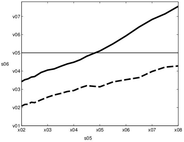
Figure 1: (a) Solid curves: accuracy ratio for our fast SVD-truncated regression algorithm, k=20k=20, p=20​ln⁡np=20\ln n. Dashed curves (for comparison): MATLAB’s svds solver which computes an approximation to the top-kk singular space; we set the error tolerance to produce comparable error to our algorithm (options.tol=0.001). The performance of our algorithm results in nearly constant error (approx 4% in the objective and 1% in the solution vector); the accuracy of svds is approximately the same but very unpredictible. (b) Ratio of the time to compute the exact solution over time to compute the approximation. For n=1500n=1500 our algorithm is about 50% more efficient. MATLAB’s svds is also more efficient asymptotically than the exact solution, but is not as efficient as our algorithm.

We perform a numerical experiment on a synthetic regression problem to illustrate the theory and the algorithm. We construct a synthetic problem as follows. We generate an n×nn\times n matrix 𝐀{\bm{\mathrm{A}}} of i.i.d. Gaussians, and set the spectral gap γk=σk+1/σk=0.99\gamma_{k}=\sigma_{k+1}/\sigma_{k}=0.99. To do this, use the SVD, 𝐀=𝐔​𝚺​𝐕T{\bm{\mathrm{A}}}={\bm{\mathrm{U}}}{\bm{\mathrm{\Sigma}}}{\bm{\mathrm{V}}}^{\textsc{T}} and rescale σk+1,…,σn\sigma_{k+1},\ldots,\sigma_{n} up or down by a constant factor so that γk=0.99\gamma_{k}=0.99. Now reconstruct 𝐀{\bm{\mathrm{A}}} using 𝐔{\bm{\mathrm{U}}}, 𝐕{\bm{\mathrm{V}}} and the rescaled 𝚺{\bm{\mathrm{\Sigma}}}. We construct the response 𝐛=𝐀k​𝐫1‖𝐀k​𝐫1‖2+0.2×𝐫2‖𝐫2‖2{\mathbf{b}}={{\bm{\mathrm{A}}}_{k}\mathbf{r}_{1}\ \over{\|{\bm{\mathrm{A}}}_{k}\mathbf{r}_{1}\|}_{2}}+0.2\times{\mathbf{r}_{2}\ \over{\|\mathbf{r}_{2}\|}_{2}}, where 𝐫1,𝐫2\mathbf{r}_{1},\mathbf{r}_{2} are random standard Gaussian vectors. So, the response 𝐛{\mathbf{b}} has roughly 80%80\% within the top-kk singular space. We set k=20k=20 and run our algorithm with p=10​ln⁡np=10\ln n. We vary n∈[100,1000]n\in[100,1000] and for each value of nn take the average over several experiments to increase statistical significance.

For comparison, we also use the truncated SVD algorithm svds distributed with MATLAB 8.1, where one can specify an error tolerance tol; svds returns 𝐔~k,𝚺~k,𝐕~k\tilde{\bm{\mathrm{U}}}_{k},\tilde{\bm{\mathrm{\Sigma}}}_{k},\tilde{\bm{\mathrm{V}}}_{k} for which ‖𝐀​𝐕~k−𝐔~k​𝚺~k‖2≤tol⋅‖𝐀‖2{\|{\bm{\mathrm{A}}}\tilde{\bm{\mathrm{V}}}_{k}-\tilde{\bm{\mathrm{U}}}_{k}\tilde{\bm{\mathrm{\Sigma}}}_{k}\|}_{2}\leq\text{\sf tol}\cdot{\|{\bm{\mathrm{A}}}\|}_{2}. The accuracy and running time results are shown in Figure 1 which illustrates the linear speedup of our algorithm. For reference, at n=1000n=1000, the exact solution takes about 2.5s on a single CPU laptop. Our algorithm performs according to the theory (with p=O⁡(ln⁡n)p=O(\ln n) we achieve approximately fixed relative error).

References

  • [1] Y. S. Abu-Mostafa, M. Magdon-Ismail, and H.-T. Lin. Learning from data. AMLBook, 2012.
  • [2] C. Boutsidis and M. Magdon-Ismail. A note on sparse least-squares regression. Information Processing Letters, 2013.
  • [3] T. F. Chan and P. C. Hansen. Some applications of the rank revealing QR factorization. SIAM Journal on Scientific and Statistical Computing, 13:727–741, 1992.
  • [4] K. R. Davidson and S. J. Szarek. Local Operator Theory, Random Matrices and Banach Spaces. In Handbook of the Geometry of Banach Spaces, volume 1. Elsevier Science, 2001.
  • [5] A. Gittens, P. Kambadur, and C. Boutsidis. Approximate spectral clustering via randomized sketching. preprint arXiv:1311.2854, 2013.
  • [6] G. Golub and C. Van Loan. Matrix computations. JHU Press, 2012.
  • [7] M. Gu and S. Eisenstat. Efficient algorithms for computing a strong rank-revealing QR factorization. SIAM Journal on Scientific Computing, 17:848–869, 1996.
  • [8] N. Halko, P.-G. Martinsson, and J. A. Tropp. Finding structure with randomness: Probabilistic algorithms for constructing approximate matrix decompositions. SIAM review, 53(2):217–288, 2011.
  • [9] P. Hansen. The truncated SVD as a method for regularization. BIT Numerical Mathematics, 27(4):534–553, 1987.
  • [10] P. C. Hansen. Truncated singular value decomposition solutions to discrete ill-posed problems with ill-determined numerical rank. SIAM Journal on Scientific and Statistical Computing, 11(3):503–518, 1990.
  • [11] R. Horn and C. Johnson. Matrix Analysis. CUP, NY, 1985.
  • [12] D. P. O’Leary and J. A. Simmons. A bidiagonalization-regularization procedure for large scale discretizations of ill-posed problems. SIAM Journal on Scientific and Statistical Computing, 2(4):474–489, 1981.
  • [13] V. Rokhlin, A. Szlam, and M. Tygert. A randomized algorithm for principal component analysis. SIAM Journal on Matrix Analysis and Applications, 31(3):1100–1124, 2009.
  • [14] A. Sankar, D. A. Spielman, and S.-H. Teng. Smoothed analysis of the condition numbers and growth factors of matrices. SIAM Journal on Matrix Analysis and Applications, 28(2):446–476, 2006.
  • [15] G. Stewart. On the perturbation of pseudo-inverses, projections and linear least squares problems. SIAM review, 19(4):634–662, 1977.
  • [16] J. M. Varah. On the numerical solution of ill-conditioned linear systems with applications to ill-posed problems. SIAM Journal on Numerical Analysis, 10(2):257–267, 1973.
  • [17] C. Vogel and J. Wade. Iterative SVD-based methods for ill-posed problems. SIAM Journal on Scientific Computing, 15(3):736–754, 1994.
  • [18] H. Xiang and J. Zou. Regularization with randomized SVD for large-scale discrete inverse problems. Inverse Problems, 29(8):085008, 2013.

Appendix A Proof of Lemma 7

The result appeared in prior work [5, Corollary 11]. Nevertheless, for completeness, we give a short, different proof based on [6, Theorem 2.6.1], which states that for any two m×km\times k orthonormal matrices 𝐖,𝐙{\bm{\mathrm{W}}},{\bm{\mathrm{Z}}} with m≥km\geq k:

‖𝐖𝐖T−𝐙𝐙T‖2=‖𝐙T​𝐖⟂‖2=‖𝐖T​𝐙⟂‖2.{\|{\bm{\mathrm{W}}}{\bm{\mathrm{W}}}^{\textsc{T}}-{\bm{\mathrm{Z}}}{\bm{\mathrm{Z}}}^{\textsc{T}}\|}_{2}={\|{\bm{\mathrm{Z}}}^{\textsc{T}}{\bm{\mathrm{W}}}^{\perp}\|}_{2}={\|{\bm{\mathrm{W}}}^{\textsc{T}}{\bm{\mathrm{Z}}}^{\perp}\|}_{2}.

𝐙⟂∈ℝm×(m−k){\bm{\mathrm{Z}}}^{\perp}\in\R^{m\times(m-k)} is such that [𝐙,𝐙⟂]∈ℝm×m[{\bm{\mathrm{Z}}},{\bm{\mathrm{Z}}}^{\perp}]\in\R^{m\times m} is a full orthonormal basis. We set 𝐔k⟂=[𝐔ρ−k,𝐔m−ρ−k]{\bm{\mathrm{U}}}_{k}^{\perp}=[{\bm{\mathrm{U}}}_{\rho-k},{\bm{\mathrm{U}}}_{m-\rho-k}].

Given some (any) 𝐒∈ℝn×k{\bm{\mathrm{S}}}\in\R^{n\times k}, recall that in our algorithm, 𝐐{\bm{\mathrm{Q}}} is obtained by a QR-factorization of (𝐀𝐀T)p​𝐀𝐒({\bm{\mathrm{A}}}{\bm{\mathrm{A}}}^{\textsc{T}})^{p}{\bm{\mathrm{A}}}{\bm{\mathrm{S}}}:

(𝐀𝐀T)p​𝐀𝐒=𝐐𝐑.({\bm{\mathrm{A}}}{\bm{\mathrm{A}}}^{\textsc{T}})^{p}{\bm{\mathrm{A}}}{\bm{\mathrm{S}}}={\bm{\mathrm{Q}}}{\bm{\mathrm{R}}}.

where 𝐐∈ℝm×k{\bm{\mathrm{Q}}}\in\R^{m\times k} and 𝐑∈ℝk×k{\bm{\mathrm{R}}}\in\R^{k\times k}. We need some basic facts:

𝐐𝐑\displaystyle{\bm{\mathrm{Q}}}{\bm{\mathrm{R}}} =\displaystyle= 𝐔k​𝚺k2​p+1​𝐕kT​𝐒+𝐔ρ−k​𝚺ρ−k2​p+1​𝐕ρ−kT​𝐒;\displaystyle{\bm{\mathrm{U}}}_{k}{\bm{\mathrm{\Sigma}}}_{k}^{2p+1}{\bm{\mathrm{V}}}_{k}^{\textsc{T}}{\bm{\mathrm{S}}}+{\bm{\mathrm{U}}}_{\rho-k}{\bm{\mathrm{\Sigma}}}_{\rho-k}^{2p+1}{\bm{\mathrm{V}}}_{\rho-k}^{\textsc{T}}{\bm{\mathrm{S}}};\ \ \ \ \ \ (9)
σk​(𝐐𝐑)\displaystyle\sigma_{k}\left({\bm{\mathrm{Q}}}{\bm{\mathrm{R}}}\right) ≥\displaystyle\geq σk​(𝐔k​𝚺k2​p+1​𝐕kT​𝐒)≥σk2​p+1​σk​(𝐕kT​𝐒);\displaystyle\sigma_{k}\left({\bm{\mathrm{U}}}_{k}{\bm{\mathrm{\Sigma}}}_{k}^{2p+1}{\bm{\mathrm{V}}}_{k}^{\textsc{T}}{\bm{\mathrm{S}}}\right)\geq\sigma_{k}^{2p+1}\sigma_{k}({\bm{\mathrm{V}}}_{k}^{\textsc{T}}{\bm{\mathrm{S}}}); (10)
σi​(𝐐𝐑)\displaystyle\sigma_{i}({\bm{\mathrm{Q}}}{\bm{\mathrm{R}}}) =\displaystyle= σi​(𝐑);\displaystyle\sigma_{i}({\bm{\mathrm{R}}}); (11)
‖𝐗𝐑‖2\displaystyle{\|{\bm{\mathrm{X}}}{\bm{\mathrm{R}}}\|}_{2} ≥\displaystyle\geq ∥𝐗∥2σk(𝐑),for any 𝐗∈ℝℓ×k.\displaystyle{\|{\bm{\mathrm{X}}}\|}_{2}\sigma_{k}({\bm{\mathrm{R}}}),\quad\text{for any }{\bm{\mathrm{X}}}\in\R^{\ell\times k}. (12)

(9) follows from a direct computation using the SVD of 𝐀{\bm{\mathrm{A}}}; (10) follows from (9) because 𝐔k{\bm{\mathrm{U}}}_{k} and 𝐔ρ−k{\bm{\mathrm{U}}}_{\rho-k} span orthogonal spaces, and the fact that the minimum singular value of a product is at least the product of the minimum singular values; (11) follows because 𝐐T​𝐐=𝐈k{\bm{\mathrm{Q}}}^{\textsc{T}}{\bm{\mathrm{Q}}}={\bm{\mathrm{I}}}_{k}; (12) is well known: it is clear if σk​(𝐑)=0\sigma_{k}({\bm{\mathrm{R}}})=0 and if σk​(𝐑)>0\sigma_{k}({\bm{\mathrm{R}}})>0 then it follows from:

‖𝐗2‖=max𝐱≠𝟎⁡‖𝐗𝐑​𝐱‖2‖𝐑​𝐱‖2≤max𝐱≠𝟎⁡‖𝐗𝐑​𝐱‖2σk​(𝐑)​‖𝐱‖2=‖𝐗𝐑‖2σk​(𝐑).{\|{\bm{\mathrm{X}}}_{2}\|}=\max_{{\mathbf{x}}\not=\bm{0}}{{\|{\bm{\mathrm{X}}}{\bm{\mathrm{R}}}{\mathbf{x}}\|}_{2}\over{\|{\bm{\mathrm{R}}}{\mathbf{x}}\|}_{2}}\leq\max_{{\mathbf{x}}\not=\bm{0}}{{\|{\bm{\mathrm{X}}}{\bm{\mathrm{R}}}{\mathbf{x}}\|}_{2}\over\sigma_{k}({\bm{\mathrm{R}}}){\|{\mathbf{x}}\|}_{2}}={{\|{\bm{\mathrm{X}}}{\bm{\mathrm{R}}}\|}_{2}\over\sigma_{k}({\bm{\mathrm{R}}})}.

Observe that 𝐔~k​𝐔~kT=𝐐𝐔𝐐T​𝐀​𝐔𝐐T​𝐀T​𝐐T=𝐐𝐐T,\tilde{\bm{\mathrm{U}}}_{k}\tilde{\bm{\mathrm{U}}}_{k}^{\textsc{T}}={\bm{\mathrm{Q}}}{\bm{\mathrm{U}}}_{{\bm{\mathrm{Q}}}^{\textsc{T}}{\bm{\mathrm{A}}}}{\bm{\mathrm{U}}}_{{\bm{\mathrm{Q}}}^{\textsc{T}}{\bm{\mathrm{A}}}}^{\textsc{T}}{\bm{\mathrm{Q}}}^{\textsc{T}}={\bm{\mathrm{Q}}}{\bm{\mathrm{Q}}}^{\textsc{T}}, because 𝐔𝐐T​𝐀​𝐔𝐐T​𝐀=𝐈k{\bm{\mathrm{U}}}_{{\bm{\mathrm{Q}}}^{\textsc{T}}{\bm{\mathrm{A}}}}{\bm{\mathrm{U}}}_{{\bm{\mathrm{Q}}}^{\textsc{T}}{\bm{\mathrm{A}}}}={\bm{\mathrm{I}}}_{k}. Therefore, using [6, Theorem 2.6.1],

‖𝐔k​𝐔kT−𝐔~k​𝐔~kT‖2\displaystyle{\|{\bm{\mathrm{U}}}_{k}{\bm{\mathrm{U}}}_{k}^{\textsc{T}}-\tilde{\bm{\mathrm{U}}}_{k}\tilde{\bm{\mathrm{U}}}_{k}^{\textsc{T}}\|}_{2} =\displaystyle= ‖𝐔k​𝐔kT−𝐐𝐐T‖2=‖𝐐T​𝐔k⟂‖2\displaystyle{\|{\bm{\mathrm{U}}}_{k}{\bm{\mathrm{U}}}_{k}^{\textsc{T}}-{\bm{\mathrm{Q}}}{\bm{\mathrm{Q}}}^{\textsc{T}}\|}_{2}={\|{\bm{\mathrm{Q}}}^{\textsc{T}}{\bm{\mathrm{U}}}_{k}^{\perp}\|}_{2} (13)
=\displaystyle= ‖(𝐔k⟂)T​𝐐‖2=‖𝐔ρ−kT​𝐐‖2.\displaystyle{\|({\bm{\mathrm{U}}}_{k}^{\perp})^{\textsc{T}}{\bm{\mathrm{Q}}}\|}_{2}={\|{\bm{\mathrm{U}}}_{\rho-k}^{\textsc{T}}{\bm{\mathrm{Q}}}\|}_{2}.\ \ \ \ \

The last equality is because 𝐔m−ρ−kT​𝐐=𝟎{\bm{\mathrm{U}}}_{m-\rho-k}^{\textsc{T}}{\bm{\mathrm{Q}}}=\bm{0} because 𝐐{\bm{\mathrm{Q}}} is in the range of 𝐀{\bm{\mathrm{A}}}. We now bound ‖𝐔ρ−kT​𝐐‖2{\|{\bm{\mathrm{U}}}_{\rho-k}^{\textsc{T}}{\bm{\mathrm{Q}}}\|}_{2}.

‖𝐔ρ−kT​𝐐𝐑‖2\displaystyle{\|{\bm{\mathrm{U}}}_{\rho-k}^{\textsc{T}}{\bm{\mathrm{Q}}}{\bm{\mathrm{R}}}\|}_{2} ≥\displaystyle\geq ‖𝐔ρ−kT​𝐐‖2​σk​(𝐑)\displaystyle{\|{\bm{\mathrm{U}}}_{\rho-k}^{\textsc{T}}{\bm{\mathrm{Q}}}\|}_{2}\sigma_{k}({\bm{\mathrm{R}}}) (14)
≥\displaystyle\geq ‖𝐔ρ−kT​𝐐‖2​σk2​p+1​σk​(𝐕kT​𝐒).\displaystyle{\|{\bm{\mathrm{U}}}_{\rho-k}^{\textsc{T}}{\bm{\mathrm{Q}}}\|}_{2}\sigma_{k}^{2p+1}\sigma_{k}({\bm{\mathrm{V}}}_{k}^{\textsc{T}}{\bm{\mathrm{S}}}).
‖𝐔ρ−kT​𝐐𝐑‖2\displaystyle{\|{\bm{\mathrm{U}}}_{\rho-k}^{\textsc{T}}{\bm{\mathrm{Q}}}{\bm{\mathrm{R}}}\|}_{2} =\displaystyle= ‖𝚺ρ−k2​p+1​𝐕ρ−kT​𝐒‖2\displaystyle{\|{\bm{\mathrm{\Sigma}}}_{\rho-k}^{2p+1}{\bm{\mathrm{V}}}_{\rho-k}^{\textsc{T}}{\bm{\mathrm{S}}}\|}_{2} (15)
≤\displaystyle\leq σk+12​p+1​σ1​(𝐕ρ−kT​𝐒).\displaystyle\sigma_{k+1}^{2p+1}\sigma_{1}({\bm{\mathrm{V}}}_{\rho-k}^{\textsc{T}}{\bm{\mathrm{S}}}).

(14) follows using (12) then (11) then (10); (15) uses (9) and submultiplicativity. Using (13) with (14) and (15), we have:

Lemma 10.

For any matrix 𝐒∈ℝn×k{\bm{\mathrm{S}}}\in\R^{n\times k},

σk​(𝐕kT​𝐒)​‖𝐔k​𝐔kT−𝐔~k​𝐔~kT‖2≤γk2​p+1​σ1​(𝐕ρ−kT​𝐒).\sigma_{k}({\bm{\mathrm{V}}}_{k}^{\textsc{T}}{\bm{\mathrm{S}}}){\|{\bm{\mathrm{U}}}_{k}{\bm{\mathrm{U}}}_{k}^{\textsc{T}}-\tilde{\bm{\mathrm{U}}}_{k}\tilde{\bm{\mathrm{U}}}_{k}^{\textsc{T}}\|}_{2}\leq\gamma_{k}^{2p+1}\sigma_{1}({\bm{\mathrm{V}}}_{\rho-k}^{\textsc{T}}{\bm{\mathrm{S}}}).

Lemma 10 holds for general 𝐒{\bm{\mathrm{S}}}. We now use the fact that 𝐒{\bm{\mathrm{S}}} is a matrix of i.i.d. standard Gaussians. Then, for any orthonormal matrix 𝐕{\bm{\mathrm{V}}}, 𝐕T​𝐒{\bm{\mathrm{V}}}^{\textsc{T}}{\bm{\mathrm{S}}} is a matrix of i.i.d standard Gaussians. So, 𝐕kT​𝐒{\bm{\mathrm{V}}}_{k}^{\textsc{T}}{\bm{\mathrm{S}}} is a k×kk\times k matrix to which Lemma 4 applies. Let 𝐕∈ℝn×n{\bm{\mathrm{V}}}\in\R^{n\times n} be the extension of 𝐕ρ−k{\bm{\mathrm{V}}}_{\rho-k} to a full orthonormal basis. Then, 𝐕T​𝐒{\bm{\mathrm{V}}}^{\textsc{T}}{\bm{\mathrm{S}}} is an n×kn\times k matrix to which Lemma 3 applies (we set t=4t=4). By a union bound, with probability at least 1−e−2​n−2.35​δ1-e^{-2n}-2.35\delta, both inequalities hold:

σk​(𝐕kT​𝐒)\displaystyle\sigma_{k}({\bm{\mathrm{V}}}_{k}^{\textsc{T}}{\bm{\mathrm{S}}}) ≥\displaystyle\geq δ​k−12;\displaystyle\delta k^{-{1\over 2}};
σ1​(𝐕ρ−kT​𝐒)\displaystyle\sigma_{1}({\bm{\mathrm{V}}}_{\rho-k}^{\textsc{T}}{\bm{\mathrm{S}}}) ≤\displaystyle\leq σ1​(𝐕T​𝐒)≤4​n1/2\displaystyle\sigma_{1}({\bm{\mathrm{V}}}^{\textsc{T}}{\bm{\mathrm{S}}})\leq 4n^{1/2}

Using Lemma 10 we conclude:

‖𝐔k​𝐔kT−𝐔~k​𝐔~kT‖2≤4​γk2​p+1​δ−1​n​k≤4​γk2​p​δ−1​n.{\|{\bm{\mathrm{U}}}_{k}{\bm{\mathrm{U}}}_{k}^{\textsc{T}}-\tilde{\bm{\mathrm{U}}}_{k}\tilde{\bm{\mathrm{U}}}_{k}^{\textsc{T}}\|}_{2}\leq 4\gamma_{k}^{2p+1}\delta^{-1}\sqrt{nk}\leq 4\gamma_{k}^{2p}\delta^{-1}n.

(We used γk≤1\gamma_{k}\leq 1 and k≤nk\leq n.) Set 4​γk2​p​δ−1​n=ε4\gamma_{k}^{2p}\delta^{-1}n=\varepsilon and solve for pp to get p=ln⁡(ε​δ/4​n)/ln⁡(γk2)p=\ln(\varepsilon\delta/4n)/\ln(\gamma_{k}^{2}), as desired.