Analysis and Control of Beliefs in Social Networks
Abstract
In this paper, we investigate the problem of how beliefs diffuse among members of social networks. We propose an information flow model (IFM) of belief that captures how interactions among members affect the diffusion and eventual convergence of a belief. The IFM model includes a generalized Markov Graph (GMG) model as a social network model, which reveals that the diffusion of beliefs depends heavily on two characteristics of the social network characteristics, namely degree centralities and clustering coefficients. We apply the IFM to both converged belief estimation and belief control strategy optimization. The model is compared with an IFM including the Barabáási-Albert model, and is evaluated via experiments with published real social network data.
Index Terms:
Complex Networks, Information Flow, Machine LearningI Introduction
Asocial network, as an abstract model of a social environment, consists of a set of nodes, which could be a set of individuals or a set of groups of individuals, and a set of relationships with specific characteristics among these nodes. There are numerous types of existing social networks in our daily lives; examples include on-line social networks such as Facebook or LinkedIn, email networks and alumni networks. Possibilities for forming new ones abound; for example, social networks among patients with a rare disease. Compared with non-social types of networks (e.g., a sensor network), social networks exhibit certain specific characteristics in quantities such as degree distributions, clustering coefficient distributions, etc. [2], [16], [18], which allow one to further analyse and control them.
Within a social network, each node has a certain belief representing its current status. The belief of a node may be influenced by other nodes connected to it, and could be changed in time. The belief may be, for example, an opinion regarding the quality of a restaurant, or the preference to attend a school [4]. In a different example, the belief may be the opinion of a patient regarding the curability of their illness. A node can propagate its belief to other connected nodes via the network links by performing certain activities, such as dining in a certain restaurant or attending a particular school, or simply by informing the other nodes. Such exposure and exchange of beliefs is actually a flow of information in a social network.
The beliefs in a social network may have value for members of the network or even outsiders. For example, knowing members’ opinions about a certain product can help a product manufacturer better predict the market and form merchandising strategies. In a clinical study, a doctor may be interested in researching ways to influence patients’ behaviour by “facilitating” interactions among patients. Consequently, prediction or even control of the beliefs in a social network can be an important and interesting problem. As such, it requires a mathematical model to simulate and analyse the flow of beliefs in a social network.
We call this model an Information Flow Model (IFM). Briefly speaking, IFM includes two main parts: a description of how beliefs are updated in time, and a description of the network structure. The first part describes how information of a member’s belief flows in the network and influences the other members. The second one describes the paths inside the network over which the beliefs can be transmitted. Details about both parts are given in Section II.
To date, research in IFMs has been mainly conducted on social learning [1], [11], [4], [7], which focuses on the first part. The effects of the second part have not received much attention, primarily due to the complexity of social network structure. Early studies on IFM had assumed acyclic networks [4], [9],[12]. More recent works adapt simple descriptions of social networks, including some limited connectivity properties [1], [11],[3],[20],[7]. Real social networks, however, have much more complicated structure, that is better captured by special network models. There are a lot of candidates of social entwork models, such as the Chung-Lu model[5], the Sznajd model[14], the Barabáási-Albert (BA) model [2] ,and the Generalized Markov Graph (GMG) model[16]. The GMG models can reveal intrinsic statistical properties of a social network (e.g., connectivity patterns, measured via distributions of centralities) and thus help analyze the information flow model.
Such intrinsic properties can (at least in theory) be exploited when one studies prediction or control problems in social networks. The properties of the network could be effectively used to determine, for example, which people should be chosen to spread the information to others in order to minimize the number of such people, maximize the number of people with the desired behaviour in the network, which is novel compared to other IFM on social networks[8], [14]. In another example, in a medical study with a limited budget, simulations of the social network could be used to select the cohort of patients in the hope of an expedited and less costly study.
In this paper, we propose an IFM with enhanced (that is, BA or GMG) models for describing the social network properties. Our motivation for proposing the specific IFM is the desire to design strategies that can control beliefs effectively, without excessive overheads in computation time or memory requirements.
The contributions of this paper are the following. First, we propose an IFM adapted to a realistic social network without excessive overheads. Second, we develop three methods to analyse beliefs in a social network; the methods can be tuned to trade off accuracy for overhead. Third, we develop strategies to control beliefs. Partial results of the paper also appeared in a brief conference paper [17]. In addition to the contents in the conference version, experiments to verify basic assumptions of models, techniques to estimate the converged beliefs as well as proofs for all the theorems and detailed description of models are added in this paper.
The paper is organized as follows. In Section II, we define the concepts of belief, control strategy and social network, and introduce the IFM formally. We introduce the notion of “control power” as a metric that can be used to compare control strategies. In Section III, we elaborate on the BA and GMG models and show how one can analytically calculate the respective control power metric. In order to verify the proposed model, we use real network data in Section IV, to test the fundamental properties of the model, and specific control strategies. We finally conclude with some remarks and future planned work in Section V.
II Information Flow Model
II-A Basic concepts in IFM
The basic elements that comprise an IFM are: the social network, the belief and the control strategy.
II-A1 Social Network
For a social network with nodes, we use indices to represent the nodes; the set of nodes is defined as: . The set of edges, , includes all pairs of connected nodes in the network, where ; the social network is thus defined as: . The social network can also be represented by its adjacency matrix A, whose elements are , where if ; otherwise.
II-A2 Belief
We employ two kinds of beliefs in the IFM model: private and updated belief. The former is unchanged and taken as an input of the model. The latter, however, is updated at each time step.
Private belief
Private beliefs abstract the intrinsic characteristics of nodes in a network. They will not be changed during the process of information flow. In this model, we assume all nodes in the network have same probabilistic distribution of private beliefs, which means node in the network takes the private belief as a random number with distribution . And we denote the private belief vector as w, whose elements are . The distribution is common knowledge to everyone in the network.
Current belief
A current belief describes the current opinion of node in a network at time step . It lies in the range . is a vector whose elements are . will be updated at each time step, and will converge to a limit in certain networks, as will be explained in Section III.
II-A3 Control Strategy
To control the overall behaviour of the network, we propose a control strategy which chooses certain nodes in the network, the so called control nodes, and asks them to broadcast certain beliefs to their neighbours.
Control Set
The set of control nodes is defined as , where , , are indices of control nodes. The uncontrolled nodes thus belong to set . And the belief chosen to be broadcast by the control node, is set to a controlled belief , where , such that:
| (1) |
for and any value of . A control strategy is specified by the control set with the corresponding controlled beliefs .
Control Power
Control power is used to measure how much the beliefs in a network have changed from their initial status. Control power for an arbitrary node is defined as the expectation of the difference between the “final” belief and the initial belief :
| (2) |
The averaged values over all nodes in the network is called the network control power:
| (3) |
II-B Information Flow Model
In an information flow model, is initialized to . The value of is then updated at each time step and determined as the average of the current beliefs of the neighbours of node , and the private belief of node , , under the influence of a control strategy. The average process is specified by an adjusted private belief vector and an adjusted adjacency matrix. The adjusted private belief vector is denoted by , with elements , where . And the adjusted adjacency matrix contains elements . The control strategy is specified by a control matrix and a control vector, which are determined by the control set and the corresponding controlled belief . The control matrix is defined as M, where if and otherwise. The control vector is V, where if , and otherwise. If , the control strategy is trivial. The updating process of the current belief vector is shown in Figure (1).
In Figure (1), the adjusted private belief and adjusted adjacency matrix are for calculating an averaged belief for each node. The control matrix M and control vector V are used to set the belief of control nodes as their corresponding controlled belief . And means the beliefs are updated based on the information of the previous time step. Equation (5) shows the formula to calculate :
| (4) |
Based on Equation (4), we can derive a compact sigma notation of current belief as shown in Equation (5):
| (5) |
assuming that the summation in Equation (5) converges to a finite matrix when approaches , the converged belief can be represented as:
| (6) |
From Equation (6) and Equation (3), we obtain the control power metric when using a control strategy with parameters M and V as11 1 is the of vector with N elements: :
| (7) |
II-C An example
In certain applications, a specific direction of change of public beliefs may be of interest, and hence a desire to control the sign of , and maximize its magnitude. For example, in a social network G the set may represent patients with certain disease, and the set may be determined by the email and phone communications between these patients. Each patient has his/her own private belief about their disease. A doctor may want to influence the beliefs of his/her patients and steer their final beliefs towards a desired belief (e.g., “following your suggested treatment will help you”). To do so, the doctor may choose several patients in the social network as control nodes , and ask them to broadcast certain controlled beliefs about taking the suggested treatment. However, the number of controlled patients may be limited by budget constraints. To reach maximum performance regarding influencing the patients beliefs, the doctor needs an optimized control strategy, as we describe later.
III Analysis of Control Power
In this section, we show how we can efficiently calculate the measure of control power in Equation (7) and select an appropriate control strategy for social networks via two social network models, the BA model and the GMG model, each of which has its own advantage in performance or resources in computation and information. We start each model by introducing the fundamental assumptions and the network synthesis processes, which will be used to verify the assumptions. The main results regarding calculation of control power are Equation (12) and Equation (18). Theorem III.3 and III.5 are the main results regarding optimization of the control power, as they provide optimized control strategies for each model.
According to Equation (7), to calculate the control power , the complete information about A is needed. In addition, the computational cost is the inversion of matrix . Such an exact solution does not shed any particular light on the choice of control set , or on the convergence speed of towards . In order to reduce the information needed to predict the control power , as well as provide a detailed analysis about the control strategy and convergence speed, network models are required. In particular, the social network models are meant to reveal the intrinsic properties of A, as the other elements in the proposed information flow model are well understood.
In practice, information about the network may not be complete, which means A is not always available. Furthermore, the network may contain a large number of nodes or edges, which requires significant computational power to process. To solve such problems, network models are necessary. A good network model can help calculate the converged beliefs using less information than A, and more efficiently. Two important network models, the BA model[2] and the GMG model[16], will be introduced and applied in the analysis of the information flow model. The reason for choosing these two models is that they both provide probabilistic properties about the element of the adjacency matrix A. The BA model assumes that only depends on the degree of nodes and , and thus requires less information. The GMG model, on the other hand, extends the dependence of to both degree and clustering coefficient of nodes and , and thus provides better accuracy.
III-A Barabáási-Albert Model
III-A1 Basic assumption
A BA model describes the growth of a network. We can, however, model a static network of interest with size as one evolves from an initial network of small size until the the number of nodes reaches . Then the network growth is freeze and we perform information flow on it. The purpose of introducing the BA model is to reveal the statistical characteristic of the adjacency matrix of a social network. The BA model, however, receives different judgements from academics[13][6], which leaves room for improvement such as the proposed GMG model.
One of the basic assumptions of the BA model is that the probability of a node attached by a new edge is proportional to its degree [2]:
| (8) |
Based on this assumption, we can derive the probability of an edge established between nodes and when the size of the network grows to a certain size, as shown in Theorem III.1. In this information flow model, is binary, so that is also the expected value of as: . Moreover, the summation of over all choices for and is , which is the summation of all degrees and is . plays an important role in the analysis of control power estimation and of control strategy, as it represents the information about the matrix A.
Theorem III.1.
In a BA model, the probability of two nodes and being connected in network with nodes and a fixed degree sequence is:
| (9) |
where is the degree corresponding to node .
III-A2 Network Synthesis
In order to verify the correctness of Equation (9), we need to generate sample social networks according to the basic assumption of the BA model. The network synthesis of a BA model is discussed in Barabáási(2002)[2]. The input of the synthesis process is the total number of nodes and the average number of edges attached to each new incoming node . The detailed process is shown in Appendix A.
III-A3 Calculation of Control Power
Theorem III.1 has revealed the statistical properties of adjacency matrix A. If we take A as a random matrix, combined with the formula to calculate a converged belief, as shown in Equation (5) and Equation (6), we are able to obtain the expected value of converged beliefs for all the nodes in the network, which is shown in Theorem III.2.
Theorem III.2.
In a BA model, the expected value of converged belief of a non-controlled node , , is:
| (10) |
where is the private belief of node , is the average number of edges per node in a network with nodes, is the degree corresponding to node , is the controlled belief of control node , is the number of control nodes, for , and is a constant which is smaller than :
| (11) |
| (12) |
The information needed for the calculation in Equatoin(12) is the degree list of network , which is far less than the information of adjacency matrix A. In addition, degree lists follow the power-law distribution in most social networks[2], which means the degree list could be sampled from the network. The computational cost of such calculation is , which is much more efficient than the matrix inverse calculation required by Equation (7).
III-A4 Optimization of Control Strategy
According to Equation (12), we can see that the control strategy, as well as the degrees of the control nodes, have a direct impact on the control power. Without loss of generality, we set the preferred sign of beliefs positive. If controlled beliefs , , are maximized to be 1, and the private belief has zero mean, then, as shown in Theorem III.3, the maximization of requires the selection of a control group to include nodes with highest degrees in the network .
Theorem III.3.
Consider a social network G of nodes, with degree list , , a private belief with zero mean and maximized control beliefs , . Suppose further that the number of control nodes, , is fixed. The control set , where if , , maximizes the control power :
| (13) |
III-B Generalized Markov Graph Model
III-B1 Basic assumption
In [16], the BA model is shown to be a special case of a Markov Graph model[10]. A Markov Graph model is based on the dependence between pairs of nodes. The basic assumption of the BA model depends however on the degree of nodes, which is a specific description of pairwise relationship between nodes. It is thus natural to extend the BA model to the GMG model to analyse the property of adjacency matrix A.
In a GMG Model, the probabilistic dependence of an edge is extended from the other attached edges to attached triangles. As degree is used to describe the dependence on attached edges, a clustering coefficient, which is related to both edges and triad relational structures, is added to the description of dependence in a GMG model. The assumption about the probability of a node attached by a new edge in a GMG model then becomes:
| (14) |
where is the degree of node , is the clustering coefficient of node , and , which is called the clustering weight, is determined by the property of the network .
The range of the clustering coefficient lies in . If there is no triangle attached to a node , the clustering coefficient will be zero. To ensure a non-zero probability of a node getting an edge, on account of a zero clustering coefficient, we adopt a in our model.
In an arbitrary network , the influence of degree and clustering coefficient on the probability of node obtaining a new edge is not equivalent. Parameter is thus used to adjust the importance of clustering coefficient versus degree. The value of changes for different types of networks and different applications.
Based on Theorem III.1, we add the influence of clustering coefficients, and to make the summation of still be the sum of degrees , the probability becomes:
| (15) |
where is:
III-B2 Network Synthesis
In order to verify the correctness of Equation (15), we need to generate sample social networks according to the basic assumption of the GMG model. In addition, the synthesized social networks can be used to estimate the clustering weight . In a GMG model[18], the input of the synthesis process is: the total number of nodes , the average number of edges attached to each node , and the clustering weight . The detailed process is shown in Appendix B.
III-B3 Calculation of Control Power
Since the GMG model makes use of more information than the BA model, the probability should be more accurately describing the statistical property of adjacency matrix A than . Based on this idea, we develop the converged belief for a GMG model, as shown in Theorem III.4.
Theorem III.4.
Define a constant as,
| (16) |
If , the expected value of converged belief of a non-controlled nodes , , in a GMG model, is,
| (17) |
where is the private belief of node in a network with nodes, is the degree corresponding to node , is the clustering coefficient of node , is the controlled belief of control node , is the number of control nodes, if , is the clustering weight for network , is defined in Equation (15).
The constant , however, will not be guaranteed to be strictly smaller than , as is in a BA model, which is shown in Appendix D. The value of will be determined by the degree list, the clustering coefficient list and the clustering weight of the network .
| (18) |
The calculation of a control power in Equation(18) requires the information of the degree list, the clustering coefficient list and the clustering weight of network . The clustering weight is obtained by a learning process, and is introduced in Section IV. When calculating the control power, the information needed by the GMG model is still far less than the information of adjacency matrix A. And due to the fact that could be rewritten as:
the computational cost of such a calculation is , which is the same as that in the BA model.
III-B4 Optimization of Control Strategy
According to Equation (18), we can see that, in addition to the control strategy and the degrees of the control nodes, the clustering coefficients of the control nodes also have a direct impact on the control power. Without loss of generality, we set the preferred sign of beliefs positive. If controlled beliefs , , are maximized to be 1, and the private belief has a zero mean, then, as we show in Theorem III.5, the maximization of requires the selection of a control group to include nodes with highest values in the network .
Theorem III.5.
Consider a social network G of nodes, with degree list , clustering weight , clustering coefficient list , , and maximized control beliefs , . Suppose further that the private belief has zero mean and the number of control nodes is fixed. Then, the control set , where if , , maximizes the control power
| (19) |
under the condition that:
| (20) |
The GMG model covers more types of social networks due to the presence of the clustering weight , an additional free parameter. Note that the range of is constrained only by the learning data set, not by the model. The specific condition in Theorem III.5 means that the optimized control strategy is appropriate only for certain types of social networks where the beliefs converge fast, as denoted by .
IV Experiments on Verification and Applications of information flow models
Three sets of experiments are described in this section. In the first set, presented in Section IV-A, we verify the basic assumptions about , the probabilistic nature of the two network models, as showed in Theorem III.1 and Equation (15). In the second set, presented in Section IV-B, we test the performance of the two social network models when the private beliefs of nodes in a social network have zero-mean. In Section IV-C, the last set of experiments compares the effects of control strategies on maximizing the control power of two different models.
Real network data[15] is used in all three types of experiments. There are different types of social networks: on-line social networks, p2p transmission networks and physicist collaboration networks. Each of these three different social networks includes several subtypes of networks. On-line social networks include Slashdot network data of August 2008 and of February 2009, Wiki-vote network data and Epinions network data. P2p transmission networks include Gnutella network data at five different times. Physicist collaboration networks include collaboration networks of physicists studying astrophysics, condensed Matter Physics, theoretical high-energy Physics, experimental high-energy Physics and general relativity. All of these effectively constitute subtypes of social networks and will be denoted by indices: . From each of these networks, we sampled 50 sub-networks using the same sampling method.
IV-A Basic Assumption Verification
The first type of experiments is designed to test the fundamental assumptions of the BA model, as shown in Section III-A1, and GMG model, as shown in Section III-B1. Both assumptions are tested on the synthesized data to show the consistence of the assumptions with the derived formula of in both models. The real network data are then used to test how computed in these two models fit into real applications. The performance of the models on synthesized data is better than that on real data, since the former were used to generate the data in the first place. The additional performance difference is due to data sampling noise as well as to the intrinsic unaccounted characteristics of the network itself.
IV-A1 Barabáási-Albert model
Verification of Theorem III.1 on synthetic data
In order to test the correctness of the basic assumption of the BA model, is computed to compare with averaged across 1,000 realizations of networks synthesized by the algorithm introduced in III-A2. An example of experimental results is shown in Figure (2) with networks containing nodes and edges. The average number of edges per node is thus . In this example, the average degree list is averaged across the degree lists of the 10,000 realizations of networks. The averaged degree list is then used to calculate as shown in Equation (9). The experiment is then repeated for different values of , and the relative error between and averaged across all pairs of nodes is shown in Table I.


| m | 1 | 2 | 3 | 4 | 5 |
|---|---|---|---|---|---|
| Relative Error | 4.32e-2 | 4.59e-2 | 3.75e-2 | 4.12e-2 | 3.61e-2 |
Performance of Theorem III.1 on real network data
In this experiment, real network samples are used to validate Theorem III.1. For each subcategory of network samples, the number of nodes is chosen to be the minimal number of nodes of all samples, which ensures the same number of samples being used for the calculation of the average number of every element in the adjacency matrix . The degree list, , and are then averaged across all samples of the same subcategory. The value of , the averaged degree list and the averaged are plugged into Equation (9) to calculate . And the value of is the average of from all 50 samples of networks belonging to the same subcategory. The relative errors between and for 14 different types of network are shown in Table II.
| On-line | P2p | Collaboration | |||
|---|---|---|---|---|---|
| Net- work | Error | Net- work | Error | Net- work | Error |
| 1 | 8.31e-2 | 5 | 22.13e-2 | 10 | 7.28e-2 |
| 2 | 8.57e-2 | 6 | 19.36e-2 | 11 | 9.15e-2 |
| 3 | 7.46e-2 | 7 | 24.18e-2 | 12 | 7.16e-2 |
| 4 | 6.59e-2 | 8 | 22.40e-2 | 13 | 8.52e-2 |
| 9 | 20.25e-2 | 14 | 9.73e-2 | ||
From Table II, we can see that the value of , according to Equation (9), is close to the expected value of in on-line social network samples and Collaboration networks. However, in p2p transmission networks, Theorem III.1 doesn’t provide a good estimate of . The main reason for the inaccurate estimation of in this case is that the degree distribution of such a network does not strictly follow the power law distribution, which means the structure of these networks is different from what the BA model can describe. This indicates that a better model is needed for a more accurate description of the real network data.
IV-A2 Generalized Markov Graph Model
Verification of basic assumption on synthetic data
The basic assumption of the GMG model is tested as follows. The number of nodes is . Five different values of : , and 4 different values of : , are chosen as the inputs of the network synthesis process introduced in III-B2. For each combination of and , is calculated and compared with averaged across 1,000 realizations of synthesized networks. The relative error between and averaged across all pairs of nodes is shown in Table III.
| 1 | 2 | 3 | 4 | 5 | |
|---|---|---|---|---|---|
| -2 | 3.25e-2 | 4.82e-2 | 4.26e-2 | 3.19e-2 | 3.55e-2 |
| -1 | 4.09e-2 | 4.91e-2 | 4.92e-2 | 3.31e-2 | 4.94e-2 |
| 1 | 4.91e-2 | 3.97e-2 | 4.60e-2 | 3.28e-2 | 3.84e-2 |
| 2 | 4.83e-2 | 4.58e-2 | 4.91e-2 | 4.31e-2 | 3.07e-2 |
Verification of basic assumptions on real network data
In this experiment, real network samples are used to validate Equation (15). For each subcategory of the network samples, the number of nodes is chosen to be the minimal number of nodes of all samples. The degree list of length , the clustering coefficient list of length , and the average number of edges are then averaged across all samples of the same subcategory. Then 25 of randomly chosen sampled networks for each sub-category of networks are used as a training set to learn the value . The rest of sampled networks are used as a test set. For each sub-category of networks, is determined as the value that generates closest to averaged across the same 25 chosen sampled networks. Next, for each sub-category of networks, averaged degree lists, average clustering coefficient lists and averaged of the other 25 sampled networks, along with the learned , are used in Equation (15) to compute . The value of is the average of over the test set for each subcategory of networks. The relative error between and for 14 different types of network is shown in Table IV.
| On-line | P2p | Collaboration | |||
|---|---|---|---|---|---|
| Net- work | Error | Net- work | Error | Net- work | Error |
| 1 | 5.14e-2 | 5 | 8.68e-2 | 10 | 5.45e-2 |
| 2 | 6.23e-2 | 6 | 7.51e-2 | 11 | 6.69e-2 |
| 3 | 4.75e-2 | 7 | 8.64e-2 | 12 | 6.28e-2 |
| 4 | 5.86e-2 | 8 | 9.13e-2 | 13 | 4.19e-2 |
| 9 | 7.26e-2 | 14 | 6.94e-2 | ||
From Table IV, we can see that the value of from Equation (9) is close to the expected value of for all three different categories of networks. Although in p2p transmission networks, Equation (9) doesn’t give as good an estimate of as in the other two categories, the overall performance of the GMG model is better than that of the BA model. Note for p2p transmission networks, whose degree distribution does not strictly follow the power law distribution, the GMG model could greatly increase the accuracy of estimate.
IV-B Converged Belief Estimation
In this experiment, we evaluate the accuracy of the converged belief estimate for both models of interest. The control strategy is set to push neutral public opinions towards positive opinions. The private beliefs of nodes in the network are set to be neutral, i.e, they obey a uniform distribution on . For both the BA and the GMG models, 25 randomly chosen networks are selected from each sub-category of networks, and used as a test set. The other 25 networks for each sub-category of networks are used as a training set for the GMG model to learn the clustering weight .
IV-B1 Barabáási-Albert Model
For each of the network samples in the test set of each sub-category of networks, a degree list is recorded. The control set is set to be the top nodes with the highest degree in the network, thus fixing the number of control nodes to: . The controlled beliefs for nodes in the control set are set to be . For each network sample, the private belief list is generated times according to a uniform distribution on .
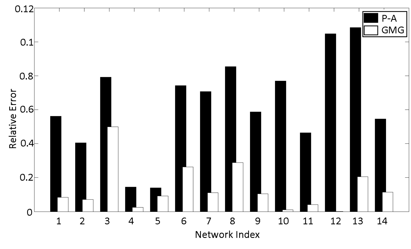
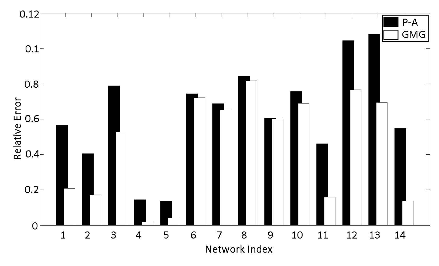
For each of the generated private belief lists, the value of control power is calculated as in Section III-A3. The same network is used for calculating the exact value of the control power according to Equation (6). The relative error between the and the exact value is then recorded as the relative error for this network sample under this belief list. The relative errors for all generated private belief lists are then averaged and recorded as the relative error of this network sample. Next, the relative errors for all network samples in the test set of each sub-category of networks are averaged and recorded as the relative error of the BA model on this sub-category. The relative errors for 14 different sub-categories of networks are shown in Figure (3) and Figure (4) to compare with the results from the GMG model.
IV-B2 Generalized Markov Graph Model
In a GMG model, the clustering weight plays a key role in describing the characteristics of the social network and has to be learned from the training data. We propose two ways to learn . The first one makes use of complete information of the adjacency matrix of the social network and provides better accuracy. The second one learns using less information, namely only the degree list and clustering coefficient list of the social network. The learned is then used to calculate the control power and the results are compared with the one from the BA model.
learning from A
The first step in a GMG model is to learn the clustering weight from the training sets for each sub-category of networks. For each training network sample, the degree list and clustering coefficient list are recorded. The control set is set to be the top nodes with highest degree in the network, and thus the number of control nodes is set to be: . The controlled beliefs for nodes in the control set are set to be , and private belief lists sampled from a uniform distribution on are obtained.
The clustering weight is chosen to minimize the difference between and . For each network sample in the training set of each sub-category of networks, the control power is calculated for each of the private belief lists with an arbitrary choice of . The exact solution of control power is also calculated for the generated private belief lists. The relative error between the and the exact value of the same private belief list is then calculated, averaged across all generated private belief lists, and recorded as the relative error for this network sample. For all network samples in the training set, the relative errors are calculated and their average value is recorded as the relative error of this sub-category of networks. The clustering weight for each sub-category of networks is chosen as the one that minimizes the relative error, as shown in Table V.
| On-line | P2p | Collaboration | |||
|---|---|---|---|---|---|
| Network | Network | Network | |||
| 1 | -1.00 | 5 | -0.20 | 10 | 1.48 |
| 2 | -1.00 | 6 | 1.29 | 11 | -2.57 |
| 3 | -0.50 | 7 | 1.52 | 12 | -2.57 |
| 4 | -0.30 | 8 | 1.45 | 13 | -2.84 |
| 9 | 1.12 | 14 | 0.52 | ||
The learned is subsequently used to test the performance of the GMG model on the test set. For each of the network samples in the test set, the degree list and the clustering coefficient list are recorded. The control set is similar to that in the training set. For each network sample, the private belief list is generated times according to a uniform distribution on . The relative errors are calculated on the test set by the same method as that used on the training set. The relative errors for 14 different sub-categories of networks are shown in Figure (3), together with the result from the BA model.
learning from the degree list and the clustering coefficient list
The second method of learning only uses partial information of the networks in the training set, i.e, the degree list and the clustering coefficient list. For each of the network samples in the training set, the number of nodes , the number of edges , the degree list and the clustering list are recorded. For an arbitrary value of , networks with nodes and edges are generated according to the network synthesis algorithm introduced in Section III-B2. For each of the generated networks, the degree list and the clustering coefficient list are recorded and averaged across these networks. The averaged degree list and clustering coefficient list are then compared with the one of the network sample in the training set. The difference between them is calculated for each of the network samples in the training set, and averaged across all networks in the training set. The that minimizes the average difference is selected as the clustering weight of this sub-category of networks. The results for all sub-categories of networks are shown in Table VI.
| On-line | P2p | Collaboration | |||
|---|---|---|---|---|---|
| Network | Network | Network | |||
| 1 | -0.40 | 5 | -0.15 | 10 | 0.58 |
| 2 | -0.30 | 6 | 0.29 | 11 | -2.30 |
| 3 | -0.40 | 7 | 0.50 | 12 | -1.50 |
| 4 | -0.20 | 8 | 0.40 | 13 | -1.70 |
| 9 | 0.10 | 14 | 0.50 | ||
The learned is then used to test the performance of the GMG model on the test set. The experiment is similar as in Section IV-B2, and the relative errors of control power are computed for all subcategories of networks, as shown in Figure (4).
Discussion of the experiments
Figures (3) and (4) indicate that the GMG model outperformed the BA model, as the former one yields smaller error for both learned from adjacency matrix and from the degree list and the clustering list. When the complete information of A of the training set is used, the learned will make the GMG model more accurate than the case when only partial information of A is learned. And the more accurate of the models, the more information is needed.
IV-C Control strategy optimization
In the experiments described in this section, we are interested in comparing the performance of control strategies under the two network models.
IV-C1 Barabáási-Albert Model
According to Theorem III.3, the control strategy of the BA model requires the control set to include the nodes with the highest degrees in the network. The test set is the same as in Section IV-B. For each network in the test set, the adjacency matrices are recorded. The indices of the first nodes with the highest degrees are set as the first nodes, so that they constitute the control set. The private belief lists with uniform distribution on are sampled times.
For the networks in the test set of each sub-category network, the converged beliefs and control power of each network are calculated according to Equation (6), based on each of the private belief lists. The control power averaged on these private belief lists and the networks is then recorded as the average control power of this sub-category of networks. The results are shown in Figure (5) and Figure (6).
IV-C2 Generalized Markov Graph Model
In a GMG model, according to Theorem III.5, the control set should include nodes with highest in order to achieve maximum control power. In this experiment, is learned from either complete or partial information of the training set. The test set is the same as that in Section IV-B. For each network in the test set, the adjacency matrix is recorded. The indices of the first nodes with highest are selected for the control set. In order to utilize all the sample networks in the test set, the ones with values that do not satisfy the condition in Theorem III.5 are also included. Note that this will yield suboptimal control power values for a GMG model. However, as the experiments show, the control strategy from the GMG model still outperforms the best one from the BA model.
The private belief lists with uniform distribution on are sampled times. For each sub-category of networks, according to Equation (6), the converged beliefs and control power of each network in the test set are calculated based on each of the private belief list for both values as shown in Table V and Table VI. The control power averaged across these private belief lists and the networks is recorded as the average control power of this sub-category of networks for each value of . The results are shown in Figure (5) and Figure (6).


From the experimental results, we can see that, with the same budget on the control set, the control strategy of the GMG model generates a higher control power than that of the BA model. Although the performance of the GMG model with partial information of the training set on control power estimation is significantly worse than the one with full information, their performance on control strategy are very close to each other.
V Conclusion and Future Research
In this paper, we introduced an information flow model to simulate the information flow in a social network. Two social network models are used to optimize the control strategy, and compute the converged beliefs of agents in a social network. Compared to a direct calculation of the converged beliefs, these two models use less information and require less computational power, but still provide results with good accuracy. In addition, the GMG Model outperforms the BA model both in belief estimation accuracy and belief control strategy, since it has a more realistic assumption and uses more information.
Future work includes better machine learning techniques for computing , potentially theoretical calculation for from network models, and more complicated information flow models. Other future open questions include temporal variability of social network features and their influence on belief estimation.
Appendix A Network Synthesis in Barabáási-Albert Model
The input of the synthesis process in the BA model is the total number of nodes and the average number of edges attached to each new incoming node . At the very beginning of the process, when the time step , there are nodes in the network and they form a fully connected network. The first node is then introduced to the network with edges attached. Each edge will choose a node to connect in the network based on its degree and clustering coefficient. At time step , when the edge of the node is seeking another node to attach to, an arbitrary node in the network is chosen with probability :
according to Equation (8). After all edges of the first node are connected to the nodes in the network, the time step changes to , and the second node is introduced. At an arbitrary time step , where , a new node is introduced to the network with edges attached. Each edge will choose a node in the network with probability proportional to . The process ends when there are nodes in the network and, the edges brought by the last node are all connected with the nodes in the network. The degree distribution of networks generated by this process will follow a power law distribution[2]. The flow chart of this process is shown in Figure (7).

Appendix B Network Synthesis in a Generalized Markov Graph Model
In a GMG model, the network synthesis includes the following steps[18]. The input of the synthesis process is: the total number of nodes , the average number of edges attached to each node , and the clustering weight . At the very beginning of the process, at time step , there are nodes in the network and they form a fully connected network. The first node is then introduced to the network with edges attached. Each edge will choose a node in the network to connect to by its degree and clustering coefficient. At time step , when the edges of the node is seeking another node to attach to, an arbitrary node in the network is chosen with probability :
according to Equation (14). After all edges of the first node are connected to the nodes in the network, the time step changes to and the second node is introduced. At an arbitrary time step , where , a new node is introduced to the network with edges attached. The edge will then choose a node in the network with probability . The process ends when there are nodes in the network and the edges brought by the last node are all connected to the nodes in the network. The degree distribution of networks generated by a GMG model can change according to the choice of value of [19]. The flow chart of this process is shown in Figure (8).

Appendix C Proof for Theorem III.1
The master equation and the solution of the master equation for the BA model is introduced in Barabáási(2002)[2]. As a reminder, we restate it here.
In a BA model, at each time step , where lies in the range , and is the highest node index at the last time step in the network, a new node with edges is added to the network. We denote this node by its joining time . The probability of an existing node in the network be connected to the new node is proportional to its degree at time . This means an increasing rate of degree of an existing node in the network is proportional to its degree, as shown in the master equation, Equation (21)[2]:
| (21) |
And the summation on the denominator of Equation (21) is known to be , as in each time step edges are added to the network. So we can rewrite Equation (21) as,
| (22) |
and the solution to this equation is[2]:
| (23) |
In the BA model, the probability of a node be connected with node is the probability of the following event happening: at time step , node is chosen to be attached to one of the edges brought by the new node. According to the basic assumption of the model and Equation (21), such a probability will be:
| (24) |
According to Equation (23), the degree of node at time step is:
| (25) |
At an arbitrary time step , the degree of node and are: and . The degree summation at time step is , which together with Equation (26) leads to:
| (27) |
If the number of nodes in the network reaches N, which means the time step is at: , and we omit the time notation for degree , we get:
| (28) |
This concludes the proof.
Appendix D Proof for Theorem III.2
According to Equation (5) and the definition of control vector V, in a network of nodes with a control strategy, the expected belief of an arbitrary non-control node , where , at an arbitrary time step , where , will be,
| (29) |
The matrix elements , with and the definition of control matrix M, can be written as:
| (30) |
To calculate the expected value of , we combine the expected value of , which equates as shown in Equation (9), together with Equation (30) to yield
| (31) |
Let
Because degree is a positive integer: , we have,
and
So and the larger of the control group is, the smaller is.
| (32) |
As , we can rewrite as and Equation (32) becomes
| (33) |
This concludes the proof.
Appendix E Proof for Theorem III.4
The proof of Theorem III.4 will be similar to that of Theorem III.2. Based on Equation (5) and the definition of control vector V, in a network of nodes with control strategy, the expected belief of an arbitrary non-control node , where , at an arbitrary time step , where , will be:
| (34) |
The matrix element , with and the definition of control matrix M, may be written as:
| (35) |
is then calculated from the expected value of , which equates as shown in Equation (15), and Equation (35):
| (36) |
Let
| (37) |
If , we can rewrite as and Equation (37) becomes
| (38) |
This concludes the proof.
Appendix F Proof for Theorem III.3
Consider an arbitrary control set with corresponding degrees . Without loss of generality, we set . For control set , the corresponding degrees satisfy if , , so, for , we have
| (39) |
Since , for , , for , according to Equation (12), can be rewritten as:
| (40) |
Since and are positive constants, the derivative of control power with respect to the degree of a controlled node is:
This concludes the proof.
Appendix G Proof for Theorem III.5
Define the weight of node as: . Consider an arbitrary control set with corresponding weight . Without loss of generality, we set . For control set , the corresponding weights satisfy if , , so, for , we have
| (44) |
Since , for , and , for , according to Equation (18) can be rewritten as:
| (45) |
where ,
,
The derivative of control power with respect to the degree of a controlled node is:
| (46) |
where ,
.
Since , we will have
| (47) |
assuming that satisfies:
| (48) |
This concludes the proof.
References
- [1] Daron Acemoglu, Munther A. Dahleh, Ilan Lobel, and Asuman Ozdaglar. Bayesian learning in social networks. Review of Economic Studies, Oxford University Press, 78(4):1201–1236, 2008.
- [2] R髱ka Albert and Albert Barabá«¡si. Statistical mechanics of complex networks. Reviews of Modern Physics, 74:47–96, January 2002.
- [3] Venkatesh Bala and Sanjeev Goyal. Learning from neighbours. The Review of Economic Studies, Vol. 65, No. 3 (Jul., 1998), pp. 595-621.
- [4] Abhijit V. Banerjee. A simple model of herd behavior. The Quarterly Journay of Economics, CVII, Issue 3, August 1992.
- [5] Fan Chung and Linyuan Lu. Complex Graphs and Networks. the AMS and CBMS, 2006.
- [6] Aaron Clauset, Cosma Rohilla Shalizi, and M. E. J. Newman. Power-law distributions in empirical data. SIAM REVIEW, Vol. 51, No. 4, pp. 661-703, 2009.
- [7] Peter Clifford and Aidan W Sudbury. A model for spatial conflict. Biometrika, 60: 581-588, 1973.
- [8] M. H. DeGroot. Reaching a consensus. Journal of the American Statistical Association, 69:118-121, 1974.
- [9] Glenn Ellison and Drew Fudenberg. Word-of-mouth communication and social learning. The Quarterly Journal of Economics, Vol. 110, No. 1 (Feb., 1995), pp. 93-125.
- [10] Ove Frank and David Strauss. Markov graphs. Journal of the American Statistical Association, 81:832–842, September 1986.
- [11] Douglas Gale and Shachar Kariv. Bayesian learning in social networks. Games and Economic Behavior, 45:329–346, November 2003.
- [12] Usman A. Khan, Soummya Kar, and Jos«± M. F. Moura. Higher dimensional consensus: Learning in large-scale networks. IEEE Transactions on Singal Processing, VOL. 58, NO. 5, MAY 2010.
- [13] Michael P. H. Stumpf and Mason A. Porter. Critical truths about power laws. Science, Vol. 335 no. 6069 pp. 665-666, February 2012.
- [14] Katarzyna Sznajd-Weron. Sznajd model and its applications. Acta Physica Polonica B, vol.36, no. 8 (2005).
- [15] StanFord University. Stanford large network dataset collection, retrieved from: http://snap.stanford.edu/data/, September 2011.
- [16] Tian Wang, H. Krim, and Y. Viniotis. A generalized markov graph model: Application to social network analysis. IEEE Journal of Selected Topics in Signal Processing, 7:318–332, April 2013.
- [17] Tian Wang and Hamid Krim. Control and prediction of beliefs on social network. IEEE International Workshop on Computational Advances in Multi-Sensor Adaptive Processing. 2013.
- [18] Tian Wang and Hamid Krim. Statistical classification of social networks. ICASSP, 2012. ICASSP.
- [19] Stanley Wasserman and Philippa Patrlson. Logit models and logistic regressions for social networks. Psychometrika, 61:401–425, September 1996.
- [20] Duncan J. Watts. A simple model of global cascades on random networks. Physical Sciences - Applied Mathematics, 99 (9) 5766-5771, 2002.
![[Uncaptioned image]](1401.0323v2/TW.png) |
Tian Wang received his B.S. (2008) degree in Physics from the University of Science and Technology of China and the M.Sc. (2011) degree in electrical engineering and Physics from North Carolina State University, where he been a Ph.D. student in Physics since 2008. His main research interest is in modelling and analysis of social network and information flow on social network. |
![[Uncaptioned image]](1401.0323v2/AK.png) |
Hamid Krim received his degrees in Electrical Engineering. As a member of technical staff at AT&T Bell Labs, he has worked in the area of telephony and digital communication systems/subsystems. In 1991 he became a NSF Post-doctoral scholar at Foreign Centers of Excellence (LSS Sup-elec/Univ. of Orsay, Paris, France). He subsequently joined the Laboratory for Information and Decision Systems, MIT, Cambridge, MA, as a Research Scientist performing/supervising research in his area of interest, and later as a faculty in the ECE dept. at North Car. State Univ. in Raleigh, N.C. in 1998. He is an original contributor and now an affiliate of the Center for Imaging Science sponsored by the Army. He also is a recipient of the NSF Career Young Investigator award. He is on the editorial board of the IEEE Trans. on SP and regularly contributes to the society in a variety of ways. His research interests are in statistical estimation and detection and mathematical modeling with a keen emphasis on applications. |
![[Uncaptioned image]](1401.0323v2/YV.png) |
Yannis Viniotis received his Ph.D. from the University of Maryland, College Park, in 1988 and is currently Professor, Department of Electrical and Computer Engineering at North Carolina State University. Dr. Viniotis is the author of over one hundred technical publications, including two engineering textbooks. He has served as the cochair of two international conferences in computer networking. His research interests include Service-Oriented Architectures, service engineering, and design and analysis of stochastic algorithms. Dr. Viniotis was the cofounder of Orologic, a successful startup networking company in Research Triangle Park, NC, that specialized in ASIC implementation of integrated traffic management solutions for high-speed networks. |