Periodic thermodynamics of isolated quantum systems

There has recently been significant progress in our understanding of statistical mechanics based on the twin concepts of equilibration, the approach of a large, closed system’s state to some steady state [8, 9, 10, 3, 12, 13, 1, 4], as well as of thermalization, when this steady state depends only upon a small number of quantities. Starting from ideas due to Jaynes [7], Srednicki and Deutsch [8, 9] and Popescu et al [16], both integrable and non-integrable closed, non-driven many-body systems have thus been shown to thermalize [4, 12, 10].

On the other hand, the study of periodically driven systems has also had a long history. Following early foundational work by Shirley [1] and Sambe [2], substantial theoretical and experimental progress has been made recently [5, 3, 4, 6, 17, 18, 19, 20, 21].

Here, we combine ideas from the two areas to extend the concept of thermalization to the out-of-equilibrium case of periodically driven systems. By devising a mapping of the system to a set of effectively non-driven systems we show that a periodically driven system asymptotically approaches a time-periodic steady state at long times (see, e.g., [22] and our Suppl. Mat.). Specializing to a large class of integrable systems, we analytically show that Jaynes’ entropy maximisation principle [7] gives a statistical mechanical description of the long-time, synchronized dynamics for infinite systems, and study the approach to this equilibrium state as a function of both the system size and time. Finally, we explain how our proposed setup is achievable with current experimental techniques.

Synchronization– The starting point for our analysis is the synchronization of the system with the driving, which may be seen as follows.

Consider a time-periodic Hamiltonian $\hat{H}(t)=\hat{H}(t+T)$ and denote the time evolution operator over a period starting from time $0\leq\epsilon<T$ by $\hat{U}\left(\epsilon,\epsilon+T\right).$ Taking $\hbar=1$, we define an effective Hamiltonian $\hat{H}_{\mathrm{eff}}$ via

$\hat{H}_{\mathrm{eff}}$ is a time-independent effective Hamiltonian which takes an initial state at $t=0$ to the same final state at $t=T$ as the real time-dependent Hamiltonian $\hat{H}(t)$.

We concentrate on “stroboscopic” observations, that is, observations at discrete points of time separated by a period, $t_{n}=\epsilon+nT$ for a given $\epsilon$. The expectation value of an arbitrary time-independent operator $\mathcal{\hat{O}}$ at time $t$, $\mathcal{O}(t)=\left<\psi(t)\right|\mathcal{\hat{O}}\left|\psi(t)\right>$, is

where $\hat{\mathcal{O}}^{(\epsilon)}=\hat{U}^{\dagger}(0,\epsilon)\hat{\mathcal{O}}\hat{U}(0,\epsilon).$ We have thus recast the time evolution into evolution under a time-independent Hamiltonian, at the price of introducing a set of new operators $\hat{\mathcal{O}}^{(\epsilon)}$.

By analogy to a static quench [1, 3] (see Supplementary Material for a discussion of the necessary conditions), one can show that each series $\{{\mathcal{O}}(t_{n});\quad n=0,1,2\ldots\}$ converges to a fixed value. This immediately implies that the long-time behaviour of the system is periodic in time, i. e., synchronised.

Construction of the periodic ensemble– We now come to the main part of our work where we show that Jaynes’ idea of entropy maximization [7, 12, 3] remains valid away from equilibrium for this class of models. In order to demonstrate that this is correct, we restrict ourselves to a class of tractable integrable Hamiltonians. For infinite systems, we show analytically that this ensemble correctly reproduces all correlation functions. For finite systems, we study the approach to the thermodynamic limit in a spatially inhomogeneous system of hard-core bosons (HCBs).

The Hamiltonians we consider are of the form

with the $\hat{a}_{i}$ fermionic or bosonic operators, $\left[a_{i},a^{\dagger}_{j}\right]_{\pm}=\delta_{i,j}$, and $\mathcal{M},\mathcal{N}$ are complex matrices. In cases of interest, the nonlinear, nonlocal transformation that brings the physical Hamiltonian to this form maps local observables to highly nonlocal, nonlinear functions of the $\hat{a}$ operators.

For Hamiltonians bilinear in the operators $\hat{a}$, $\hat{H}_{\mathrm{eff}}$ are bilinear and may therefore be brought to the form

by a unitary transformation ($L$ is the system size). The operators $\hat{\mathcal{I}}_{p}(t):=\hat{U}(0,t)\tilde{a}^{\dagger}_{p}\tilde{a}_{p}\hat{U}^{\dagger}(0,t)$ (of which there are $L$) correspond to conserved quantities, $\left<\psi(t)\right|\hat{\mathcal{I}}_{p}(t)\left|\psi(t)\right>=\left<\psi(0)\right|\hat{\mathcal{I}}_{p}(0)\left|\psi(0)\right>$ for all $t$, and are temporally periodic.

Operator $\hat{\rho}_{PGE}(t)$ has the following two properties: First, it correctly gives the conserved quantities: $\mathrm{tr}\left(\tilde{a}^{\dagger}_{p}\tilde{a}_{q}\hat{\rho}_{PGE}(t)\right)=\delta_{p,q}\left<\psi(t)\right|\hat{\mathcal{I}}_{p}(t)\left|\psi(t)\right>$. Secondly, since the $\hat{\mathcal{I}}_{p}$ are periodic in time, it is itself manifestly periodic with time: $\hat{\rho}_{PGE}(t)=\hat{\rho}_{PGE}(t+T)$.

Finally we can analytically show that the PGE density matrix exactly reproduces all correlation functions in the thermodynamic limit; this somewhat lengthy but ultimately elementary calculation is described in the Supplementary Material. This constitutes our central conceptual result.

Application to Finite Systems: Numerical Results – Let us now supplement the above exact and general results using numerical simulations for specific, finite systems. While the proof for the correctness of the PGE is strictly applicable only in the thermodynamic limit, we shall see that the deviation of finite systems from the PGE result rapidly decreases with system size.

A number of different physical systems may be mapped to Eq. (14) (see Supplementary Material). Here we present numerical results for the experimentally relevant case of HCBs subject to a simple potential, the Hamiltonian for which reads

with the $\hat{b}_{i}$ HCBs. The HCBs are described by operators $\hat{b}$ obeying bosonic commutation relations, $\left[\hat{b}_{i},\hat{b}_{j}^{\dagger}\right]=\delta_{i,j}$, with the addional hard-core condition $\hat{b}^{2}_{i}=0$. A Jordan-Wigner transformation, $\hat{b}_{i}=\hat{a}_{i}\prod_{j<i}(-1)^{\hat{n}_{j}}$ with $\hat{n}_{j}=\hat{b}_{j}^{\dagger}\hat{b}_{j}=\hat{a}_{j}^{\dagger}\hat{a}_{j}$, maps $\hat{H}_{b}(t)$ to Eq. (14) with $\mathcal{M}_{i,j}(t)=-\frac{1}{2}J_{i}(t)\left(\delta_{i+1,j}+\delta_{i-1,j}\right)+\delta_{i,j}V_{i}(t)$, $\mathcal{N}_{i,j}=0$ and fermionic commutation relations for the $\hat{a}$.

Here we focus on a time-dependent superlattice potential superposed on a quadratic potential, $V_{i}(t)=\frac{1}{2}\left(\left(i-L/2\right)/\ell_{ho}\right)^{2}+\Delta(-1)^{i}\cos\left(\omega t\right)$ and a time-dependent hopping amplitude $J_{i}(t)=J+\delta J\cos(\omega t)$ with $\omega=2\pi/T$. The protocol we use is to prepare the system in the ground state in the presence of a harmonic potential $V^{(0)}_{i}=\frac{1}{2}\left(\left(i-L/2\right)/\ell_{ho}\right)^{2}$, fixing $\ell_{ho}=N$. This allows us to take the thermodynamic limit, since for large total number of particles the dimensionless parameter [28] $\tilde{\rho}=N_{b}/\ell_{ho}$ plays a role analogous to the density in the uniform limit. Results with different system sizes but constant $\tilde{\rho}$ are therefore comparable.

At time $t=0$, the driving is switched on so that the total Hamiltonian is $\hat{H}_{b}(t)=-\frac{1}{2}J\sum_{i}\hat{b}^{\dagger}_{i}\hat{b}_{i+1}+\mathrm{hc}+\sum_{i}V_{i}(t)\hat{b}^{\dagger}_{i}\hat{b}_{i}$ with $V_{i}(t)=V^{(0)}_{i}+\Delta(-1)^{i}\cos\left(2\pi t/T\right)$.

Concentrating on the experimentally accessible momentum distribution of the bosons, $\hat{n}^{(b)}(k)=L^{-1}\sum_{i,j}\hat{b}^{\dagger}_{i}\hat{b}_{j}\exp(-2\pi k(i-j)L^{-1})$ we use the numerical method used in, inter alia, [29]; it consists of solving the fermionic time-dependent problem and, at the end, inverting the Jordan-Wigner transformation.¹¹ 1 It is worth pointing out that $\hat{n}^{(b)}$ for the bosons is neither bilinear nor local in terms of the Jordan-Wigner fermions, since $\hat{b}^{\dagger}_{i}\hat{b}_{j}=\hat{a}_{i}^{\dagger}\left(\prod_{i\leq m<j}(-1)^{\hat{n}_{m}}\right)\hat{a}_{j}$. We therefore expect the PGE predictions to only approximate the real dynamics, becoming exact at the thermodynamic limit.

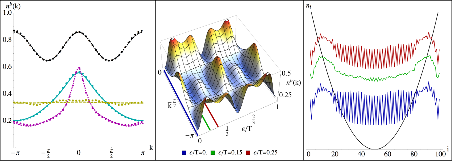
We begin by demonstrating a number of possible periodic states, corresponding to different parameters of the model. The leftmost panel of Figure 1 shows snapshots of the PGE momentum distribution $\mathrm{tr}\left(\hat{\rho}_{PGE}\hat{n}^{(b)}(k)\right)$ at the beginning of each period ($\epsilon=0$) for different parameter values. We emphasise that, away from the high-frequency regime, the corresponding time-averaged Hamiltonian [5, 23] is not an appropriate description. As a striking example, the black line shows a momentum distribution with peaks at the edges of the Brillouin zone. Concentrating now on the parameters corresponding to the cyan line, the central panel shows the time evolution of the momentum distribution over an entire period. Note, the system evolves through states in which the momentum is peaked at different locations of the Brillouin zone. Finally, the rightmost panel shows three snapshots of the density distribution of the same system at times indicated by the coloured lines in the central panel. The high spatial frequency oscillations and the peaking of the density at the edges is also very different from what would be obtained had the system been well-described by a time-averaged Hamiltonian, since the time-averaged potential (shown in black) is smooth and its potential highest at the edges.

We next discuss the approach to the long-time periodic state as a function of time and system sizes. After showing that the stroboscopic values of observables approach, then oscillate around, a constant value for each $\epsilon$, we proceed to demonstrate that both this average value and the relative magnitude of the oscillations away from it decay to zero with increasing system size, in agreement with our analytical results for infinite systems. The approach is rapid: within a few periods, the system is practically thermalized.

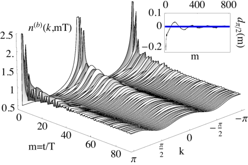
The main plot of Fig. 2 shows the stroboscopic approach to the PGE state of the full bosonic momentum distribution, $\hat{n}^{(b)}(k,mT)$, for the parameters corresponding to the black line in Fig. 1. The entire momentum distribution approaches, then oscillates around, a period-independent result. The inset focusses on the component $\hat{n}^{(b)}(k=\pi/2)$, showing the stroboscopic time evolution of its difference from the value predicted by the PGE as a function of period, showing the oscillations about the equilibrium value shown by the heavy blue lines.

We now quantitatively study the approach to the PGE limit as system size is increased. In Fig. 3 we plot the average of the distance of the dynamical momentum distribution from its PGE value over a number of periods, $\overline{d}=(LN)^{-1}\sum_{m=n}^{n+N}\sum_{k}\left|\hat{n}^{(b)}(k,mT)-\hat{n}_{PGE}(k)\right|$, as a function of the inverse system size $1/L$. These plots are for large $n=40L$ and $N=20L$ in order to to allow plenty of time for equilibration. From Fig. 3, we conclude that the average of the momentum distribution approaches the PGE result, while fluctuations away from it average become smaller with increasing system size: as $L\rightarrow\infty$, the momentum distribution rapidly approaches the PGE periodic steady-state.

In conclusion, we have shown that the real dynamics rapidly approaches the thermodynamic-limit and long-time results for relatively small systems and short times.

Experiments–We now turn to the question of the experimental implementation of the specific system we have studied. To realize our proposal, three ingredients are required: A superlattice potential, periodic modulation and HCBs.

Experiments using a superlattice potential are already available [24], while periodic modulation of the lattice depth [17, 25, 17] is a standard technique. In particular, periodically driving a superlattice potential is described in Ref. [20]. Finally, the HCB regime may be achieved via confinement-induced resonance, which involves manipulating the radial harmonic potential strength [26, 27].

The example we have studied above is therefore accessible with current experimental techniques.

Conclusions and outlook–For a large class of integrable periodically-driven systems, we have shown that a periodic steady-state is attained at long times. To describe this state, we have constructed a periodic version of the generalized Gibbs ensemble (GGE) [12], commonly introduced in connection with quenches in integrable models. We have provided an analytical demonstration that it exactly reproduces the periodic steady-state in the thermodynamic limit. We also provide numerical evidence of rapid convergence (i) to the thermodynamic-limit prediction with increasing system size and (ii) to the steady-state with time.

It would be natural to extend our results to a generic nonintegrable situation. Our PGE is analogous to the GGE for non-driven systems [12]; the analogy would suggest that, for a closed, non-integrable, periodically-driven system, a subsystem for which the rest of the system plays the role of a bath might be described by the periodic density matrix operator $\exp\left(\hat{H}_{\mathrm{eff}}\left(\epsilon\right)=\hat{U}\left(0,\epsilon\right)\hat{H}_{\mathrm{eff}}\hat{U}^{\dagger}\left(0,\epsilon\right)\right)$, analogous to the Gibbs ensemble for non-driven systems [16]. Unfortunately, there are several issues with this; chief amongst them are that $\hat{H}_{\mathrm{eff}}\left(\epsilon\right)$ is not a local operator in general and, more seriously, that $\hat{H}_{\mathrm{eff}}\left(\epsilon\right)$ is not uniquely defined (its eigenvalues are only defined modulo $2\pi/T$–we do not use the eigenvalues and therefore circumvent this problem in our work). We are currently investigating possible resolutions of these conceptual issues.

Our work here should be compared to the usual situation for out-of-equilibrium systems, where each case has to be studied individually using ad-hoc techniques tailored to the specific problem at hand. In contrast, for this type of periodically-driven systems the general framework of maximum entropy statistical mechanics applies as-is. It not only gives the correct ensemble but also allows detailed computation of physical observables. We hope that this work will motivate the search for further such “thermodynamic” principles governing driven systems in all generality.

Supplementary material for “Periodic thermodynamics of isolated quantum systems” Achilleas Lazarides¹, Arnab Das^1,2 and Roderich Moessner¹ August 24, 2026

References

- [1] J. H. Shirley, Phys. Rev. 138, B979 (1965).
- [2] H. Sambe, Phys. Rev. A 7, 2203 (1973).
- [3] M. Grifoni and P. Hanggi, Physics Reports 304, 229 (1998).
- [4] A. Das, Phys. Rev. B 82, 172402 (2010).
- [5] A. Eckardt, C. Weiss, and M. Holthaus, Phys. Rev. Lett. 95, 260404 (2005).
- [6] N. H. Lindner, G. Refael, and V. Galitski, Nature Physics 7, 490 (2011).
- [7] E. T. Jaynes, Phys. Rev. 106, 620 (1957).
- [8] M. Srednicki, Physical Review E 50, 888 (1994).
- [9] J. M. Deutsch, Phys. Rev. A 43, 2046 (1991).
- [10] M. Rigol, V. Dunjko, and M. Olshanii, Nature 452, 854 (2008).
- [11] M. A. Cazalilla, A. Iucci, and M.-C. Chung, Phys. Rev. E 2012, 011133 (2012).
- [12] M. Rigol, V. Dunjko, V. Yurovsky, and M. Olshanii, Phys. Rev. Lett. 98, 050405 (2007).
- [13] P. Calabrese, F. H. L. Essler, and M. Fagotti, Phys. Rev. Lett. 106, 227203 (2011).
- [14] P. Reimann, Phys. Rev. Lett. 101, 190403 (2008).
- [15] M. Fagotti and F. H. L. Essler, Phys. Rev. B 87, 245107 (2013).
- [16] S. Popescu, A. J. Short, and A. Winter, Nature Physics 2, 754 (2006).
- [17] T. Stöferle, H. Moritz, C. Schori, M. Köhl, and T. Esslinger, Phys Rev. Letters 92, 130403 (2004).
- [18] H. Lignier, A. Zenesini, D. Ciampini, O. Morsch, E. Arimondo, S. Montangero, G. Pupillo, and R. Fazio, Phys. Rev. A 79, 041601 (2009).
- [19] E. Haller, M. Gustavsson, M. J. Mark, J. G. Danzl, R. Hart, G. Pupillo, and H.-C. Naegerl, Science 325, 1224 (2009).
- [20] T. Iadecola, C. Chamon, R. Jackiw and S.-Y. Pi, Phys. Rev. B 88, 104302 (2013).
- [21] Y.-A. Chen, S. Nascimbène, M. Aidelsburger, M. Atala, S. Trotzky, and I. Bloch, Phys. Rev. Lett. 107, 210405 (2011).
- [22] A. Russomanno, A. Silva, and E. Santoro, Phys. Rev. Lett. 109, 257201 (2012).
- [23] A. Eckardt, M. Holthaus, H. Lignier, A. Zenesini, D. Ciampini, O. Morsch, and E. Arimondo, Phys. Rev. A 79, 013611 (2009).
- [24] M. Atala, M. Aidelsburger, J. T. Barreiro, D. Abanin, T. Kitagawa, E. Demler, and I. Bloch, Nature Physics 9, 795 (2013).
- [25] E. Haller, R. Hart, M. J. Mark, J. G. Danzl, L. Reichsöllner, M. Gustavsson, M. Dalmonte, G. Pupillo, and H. C. Nägerl, Nature 466, 597 (2010a).
- [26] M. Olshanii, Phys. Rev. Lett. 81, 938 (1998).
- [27] E. Haller, M. J. Mark, R. Hart, J. G. Danzl, L. Reichsöllner, V. Melezhik, P. Schmelcher, and H. C. Nägerl, Phys. Rev. Lett. 104, 153203 (2010b).
- [28] M. Rigol and A. Muramatsu, Phys. Rev. A 70, 031603 (2004).
- [29] M. Rigol and A. Muramatsu, Mod. Phys. Lett. B 19, 861 (2005).
- [1] P. Reimann, Phys. Rev. Lett. 101, 190403 (2008).
- [2] P. Reimann and M. Kastner, New. J. Phys. 14, 043020 (2012).
- [3] M. A. Cazalilla, A. Iucci, and M.-C. Chung, Phys. Rev. E 2012, 011133 (2012).
- [4] M. Fagotti and F. H. L. Essler, Phys. Rev. B 87, 245107 (2013).
- [5] B. Dóra, A. Bácsi, and G. Zaránd, Phys. Rev. B 86, 161109 (2012).
- [6] L. D. Landau and E. M. Lifshitz, Statistical Physics, Vol. 2 (Pergamon Press, Oxford, 1980).
- [7] S. Ziraldo, A. Silva, and G. E. Santoro, Phys. Rev. Lett. 109, 247205 (2012).
- [8] S. Ziraldo and G. E. Santoro, Phys. Rev. B 87, 064201 (2013).
- [9] F. D. M. Haldane, Phys. Rev. Lett. 47, 1840 (1981).
- [10] T. Giamarchi, Quantum Physics in One Dimension (Clarendon Press, Oxford, 2003).
- [11] M. A. Cazalilla, J. Phys. B 37, S1 (2004).
- [12] B. Dora, M. Haque, and G. Zaránd, Phys. Rev. Lett. 106, 156406 (2011).
- [13] X.-G. Wen, Quantum Field Theory of Many-Body Systems (Oxford University Press, Oxford, 2004).
- [14] D. M. Gangardt and G. V. Shlyapnikov, Phys. Rev. Lett. 90 (2003).
- [15] A. Lazarides, O. Tieleman, and C. Morais Smith, Phys. Rev. A 84, 023620 (2011).