A meta-analysis of parton distribution functions
Abstract
A “meta-analysis” is a method for comparison and combination of nonperturbative parton distribution functions (PDFs) in a nucleon obtained with heterogeneous procedures and assumptions. Each input parton distribution set is converted into a “meta-parametrization” based on a common functional form. By analyzing parameters of the meta-parametrizations from all input PDF ensembles, a combined PDF ensemble can be produced that has a smaller total number of PDF member sets than the original ensembles. The meta-parametrizations simplify the computation of the PDF uncertainty in theoretical predictions and provide an alternative to the 2010 PDF4LHC convention for combination of PDF uncertainties. As a practical example, we construct a META ensemble for computation of QCD observables at the Large Hadron Collider using the next-to-next-to-leading order PDF sets from CTEQ, MSTW, and NNPDF groups as the input. The META ensemble includes a central set that reproduces the average of LHC predictions based on the three input PDF ensembles and Hessian eigenvector sets for computing the combined PDF+ uncertainty at a common QCD coupling strength of 0.118.
Keywords:
Global QCD analysis, parton distributions, Large Hadron Colliderpacs
14.65.Dw, 12.38.-tI Introduction
Parton distribution functions (PDFs) in the nucleon describe long-distance nonperturbative effects in high-energy QCD processes. Their detailed understanding is vital for the physics program at the Large Hadron Collider (LHC). First years of the LHC operation have culminated in the discovery of a Higgs scalar particle [1, 2] and tested various Standard Model processes at the highest precision ever attained. No direct indications for physics beyond the Standard Model have been found so far, yet future plans [3] envision reaching much higher accuracy in new physics searches at the raised LHC energy in the next decade. Toward this goal, many theoretical predictions for the LHC must include next-to-next-to-leading order (NNLO) QCD and next-to-leading order (NLO) electroweak contributions, as well as parametrizations for nonperturbative PDFs of comparable accuracy. Modern PDFs are determined by several groups from a statistical analysis of multiple hadronic experiments utilizing diverse methods. In this paper, we discuss estimation of the full uncertainty in QCD predictions based on the combination of inputs from PDFs by several groups. The combination of PDF uncertainties is non-trivial, given a variety of considerations that go into their estimation, and has important implications for those LHC measurements where the PDF uncertainty results in a leading systematic error.
Recent NNLO PDF parametrizations include CT10 [4], MSTW 2008 [5], and NNPDF 2.3 [6], determined from the global analysis of hadronic data; ABM11 [7], ABM12 [8], and JR09 [9, 10], determined from the analysis of deep-inelastic scattering (DIS) and vector boson production; and HERAPDF 1.5 [11], determined solely based on DIS. Every group provides an ensemble of error PDF sets, besides the central PDF set, to compute the PDF uncertainty according to the Hessian [12, 13] or Monte-Carlo sampling methods [14, 15].** * Throughout the paper, we draw a distinction between the “PDF sets” and “PDF ensembles”. A “PDF set” is a group of parametrizations of PDFs for various flavors (, , etc.) corresponding to one point in the PDF parameter space. The “PDF ensemble” is a group of PDF sets from several points in the parameter space, such as in the “CT10 ensemble of 51 PDF error sets”. The central PDFs and PDF error bands at the 68% confidence level (c.l.) from CT10, HERAPDF1.5, MSTW’08, and NNPDF2.3 ensembles are similar, but not exactly identical [16]. These PDF ensembles may share some common ingredients, like using the same experimental data sets or analogous statistical methods. They also exhibit substantial differences, notably in the choice of the QCD coupling strength, heavy-quark masses and heavy-quark schemes, PDF functional forms, and error propagation. There are also many other specialized PDFs, e.g., CJ12 [17], PDFs with intrinsic charm [18, 19] and photons [20, 21], SOM PDFs [22], and nuclear PDFs [23, 24, 25, 26].
When predicting a new QCD observable , a user may estimate the full uncertainty due to the PDFs by repeatedly computing for every provided error PDF set and combining all such predictions according to a prescribed formula. Such estimation may cause a practical bottleneck if is a complex observable that must be recomputed with hundreds of PDF parametrizations.
A related difficulty concerns combination of estimated PDF uncertainties on using PDFs from several ensembles. Various groups follow incongruous procedures when defining their PDF uncertainties, which must be somehow reconciled in order for the combination to proceed. The PDF4LHC study recommended in 2010 [27, 28] to find the combined 68% c.l. uncertainty for using NLO PDFs from three groups (CT, MSTW, and NNPDF) by first calculating the 68% c.l. interval independently for each group and in accordance with the definition that the group had adopted; and then taking an envelope of the three 68% c.l. intervals as the total uncertainty. Later, this procedure was applied to the NNLO PDFs [16]. The resulting estimate of the PDF uncertainty spans all individual confidence intervals obtained under non-identical definitions.
A related combination method [29, 30] (which will be referred to as a ’replica combination method’) estimates the total PDF uncertainty by combining Monte-Carlo replicas (random PDF error sets) generated from the input PDF ensembles. To carry out this approach, each input ensemble utilizing the Hessian method is first converted into a secondary Monte-Carlo ensemble with about 100 member sets that is then merged with the rest of the Monte-Carlo ensembles. When CT10, MSTW’08, and NNPDF2.3 ensembles are combined, the total PDF uncertainty in the replica combination method is close to that derived according to the PDF4LHC recommendation. In either the PDF4LHC or replica combination method, the number of the final PDF error sets turns out to be the same or even larger than the number of the input sets, which is in the range of hundreds when predictions from many groups are combined. Both methods estimate for multiply redundant PDF sets, many of which predict the values that are close to the central prediction and contribute little to the total uncertainty.
We will now outline an alternative approach called a “meta-analysis” in which the input PDF sets are combined before the observable is computed. Each member set of the initial PDF ensembles is approximated at an energy scale by an intermediary functional form dependent on PDF parameters The distribution of the member sets over the parameters is analyzed, and a hypervolume spanning parameters of all PDF error sets is determined. Finally, using the shared parametrization form, we can construct a relatively small number of PDF eigenvector sets spanning all 68% c.l. error sets using the Hessian or Monte-Carlo sampling method. When the input PDF ensembles are statistically consistent with one another, the new PDF error sets reproduce the average and total PDF uncertainty of the initial PDF sets, but the number of the independent sets can be considerably reduced in the new ensemble.
The final ensemble of META PDFs constructed this way serves the same purpose as the PDF4LHC and replica combination methods, yet it combines the PDFs directly in the PDF parameter space while at the same time minimizing numerical computation efforts. In general it is difficult to bring all diverse PDFs into a common framework, for example because distinct heavy-quark schemes are used at momentum scales of a few GeV. But for purposes of the LHC studies, and focusing only the and ranges corresponding to the LHC kinematics, most of the difficulties can be circumvented by requiring the lowest scale for the PDF evolution to be above the bottom quark mass, where all PDF sets evolve assuming the same number of active flavors. The effects of choosing different heavy-quark schemes are then taken into account through the boundary conditions at the low scale . A variety of checks is performed to guarantee that the physics inputs and statistical features of the input PDF sets are preserved by the META PDF ensemble.
In the next sections, we build a combined ensemble of NNLO META PDFs for LHC studies from CT10, MSTW 2008 and NNPDF2.3 ensembles with 5 active quark flavors. These ensembles use compatible central values of the QCD coupling (), similar data sets and procedures, and are in quantitative agreement [16]. The combination of such compatible sets is the simplest one to carry through, but the framework of the meta-analysis does not limit the number of the PDF ensembles that can be combined. We also derive and examine the meta-parametrizations for the ABM11 and HERAPDF1.5 sets that were not included in the PDF4LHC combination. The ABM and HERAPDF ensembles are quite distinct from the three global ensembles, hence we cannot include them into the META ensemble yet using the combination procedure that was chosen. We comment on the comparison of the ABM and HERAPDF ensembles with the META PDFs in later sections.
The paper is organized as follows. Section II introduces the meta-parametrizations to approximate the input PDFs at energies relevant for the LHC. Section III constructs a META PDF ensemble from CT10, MSTW’08, and NNPDF2.3 NNLO ensembles. In Section IV we briefly discuss phenomenological applications of the META PDFs. Section V contains a short summary.
II Meta-parametrizations for input PDFs
| Input PDF ensemble | Ref. | Initial | Analysis | Error | Free | Error | Included | |
| scale | type | type | parameters | sets | in META PDFs | |||
| CT10 | [4] | 1.3 GeV | 0.118 | Global | Hessian | 25 | 50 | Yes |
| MSTW’08 | [5] | 1.0 GeV | 0.11706 | Global | Hessian | 20 | 40 | Yes |
| NNPDF2.3 | [6] | 1.414 GeV | 0.118 | Global | MC | 259 | 100 | Yes |
| ABM11() | [7] | 3.0 GeV | 0.118 (0.1134) | DIS+DY | Hessian | 29 | 28 | No |
| HERAPDF1.5 | [11] | 1.378 GeV | 0.1176 | DIS | Hessian | 14 | 28 | No |
II.1 Selection of input PDF ensembles
In a general-purpose PDF ensemble, parton distributions are parametrized by certain functions of the partonic momentum fraction at an initial scale of order 1 GeV and found numerically at higher scales by solving QCD evolution equations. The PDF depends on the flavor of the probed parton, but we omit the index in to simplify the notation, assuming that all considerations apply to every parton flavor.
At low scales comparable to the charm and bottom masses, the PDFs from various groups cannot be directly combined because of different implementations of heavy-quark mass contributions. In typical LHC applications, on the other hand, the hard factorization scale tends to be well above the bottom quark mass GeV. At such scales the PDFs from all groups evolve in the same way according to the DGLAP evolution equations with 5 active quark flavors. At even higher scales, , masses of charm and bottom quarks can be neglected in hard-scattering contributions. We therefore can circumvent explicit treatment of heavy-quark effects by approximating the PDFs by flexible meta-parametrizations at a scale above . For definiteness we choose GeV and assume 9 independent PDF parametrizations at this scale, for , , , , , , , , and . We neglect small differences between and , and and PDFs.
The input PDF ensembles that will be considered in this analysis are summarized in Table 1. They are obtained at the next-to-next-to-leading order (NNLO) in the QCD coupling strength . Every ensemble except ABM11 includes 28-100 PDF error sets probing the uncertainty due to the PDF parametrization at a fixed close to 0.118, as well as additional best-fit PDF parametrizations for alternative to examine the magnitude of the uncertainty. The 0.118 value is compatible with the world-average QCD coupling [31] and will be used as a common value in most comparisons. In the ABM11 ensemble, the error PDFs are given for a lower central value of and include the variation in the covariance matrix. An update of the ABM11 analysis tuned to the LHC data, called ABM12, has been released very recently [8]. Only the ABM11 ensemble provides a member set for from their series (but not the PDF error sets at this ). Because the ABM error sets correspond to a lower value, they should not be compared on the same footing with the error PDFs for a fixed from the other groups. For this comparison, we will examine the meta-parametrization for the ABM11 member set at , as well as LHC predictions for ABM12 using the central . Note that, for making theoretical predictions, the ABM group recommends to use their PDF sets corresponding to their best-fit .
When combining the PDF ensembles, one follows two common methods used for estimating the PDF uncertainty, the Hessian method [12, 13] and the Monte Carlo (MC) sampling method [14, 15]. We summarize the core relations of the two methods for completeness. Generally speaking, the Hessian approach provides PDF error sets (called “eigenvector sets”) that only estimate a given confidence interval for the PDFs without specifying the actual probability distribution. The MC method returns PDF error sets called “replicas” to estimate the probability density for the desired QCD observable.
The following simplest statistics can be computed with either method.
- 1.
The central prediction for a QCD observable , such as a cross section or the PDF itself, is the value given by the most probable PDF in the Hessian approach (corresponding to the lowest log-likelihood in the global fit); or the mean value of predictions from all the replicas in the MC method.
- 2.
The PDF uncertainty in the Hessian method estimates the boundaries of the confidence interval on , usually at the 68% or 90% c.l. Both the symmetric [12, 13] uncertainty, , and asymmetric uncertainties [32] can be estimated:
(1) (2) (3) where are the values of corresponding to the upper and lower boundary of the confidence interval for the parameter . These formulas are used by the CTEQ, HERA, and MSTW groups, while the ABM group uses a variant of the Hessian master formula that estimates the symmetric uncertainty from the differences between the predictions based on the central PDF and one error set for each eigenvector direction [7].
In the MC approach, the symmetric 68% c.l. PDF uncertainty is given by a standard deviation :
(4) - 3.
The tolerance (error) ellipse is introduced to study correlations between two observables, e.g., and . In the Hessian approach, we first define the correlation angle as [12, 32, 33]
(5) The tolerance ellipse is the projection onto the plane of the Hessian hypersphere spanned by the eigenvector sets in the linear approximation for PDF dependence of and . The ellipse can be found from the parametric equations
(6) for .
In the MC approach we can also define the error ellipse by an equation
(7) where is the correlation of and , and
(8) Projections of the ellipse on the and axes coincide with the confidence intervals on and determined by , for instance (1.64) for the 68 (90)% c.l. Eqs. (5) and (7) delineate the regions of the prescribed confidence when the distributions of and are close to Gaussian ones. The equivalence of the Hessian and MC error ellipses in the Gaussian case can be demonstrated by identifying .


II.2 Parametrization and sum rules
The functional forms for are often assumed to behave as in the and limits on the basis of Regge and quark counting arguments. They must satisfy the valence quark number and momentum sum rules and predict positive cross sections. The free parameters of are found from a fit, their total number is chosen so as to provide very flexible functional forms agreeing with the data, but without overfitting the data. NNPDF2.3 uses a neural network with 259 parameters to minimize the parametrization bias, while the CT10 and MSTW’2008 NNLO ensembles keep 25 and 20 free parameters, respectively. Another convenient form utilizes Chebyshev orthogonal polynomials [34, 35, 36]. This form is particularly suited for constructing the meta-parametrizations and will be employed in our analysis.


In those ranges where the experimental data impose tight constraints, the number of effective degrees of freedom is smaller than in the full PDF ensemble, so a smaller number of parameters is needed to approximate the acceptable PDF shapes. We will therefore fit the effective parametrizations to the input PDFs only in the ranges where sufficient experimental constraints are available. The boundaries of these ranges are taken to satisfy for all quark flavors; for the gluon and quarks; for quarks; and for quarks. By construction, the uncertainty bands of the input PDFs and their meta-parametrizations agree well in the fitted regions. Outside these ranges, the meta-parametrizations are determined by extrapolation and span a wide uncertainty band, which is close, although not identical, to the original PDF uncertainty (which has a large uncertainty of its own at such ). The PDFs in the outside (unfitted) regions are hardly constrained at the moment and have negligible contributions to most LHC observables even at 14 TeV.


The specific effective form that we choose at the scale for each flavor is
| (9) |
It satisfies the above asymptotic behaviors, at and at , while the detailed shape is regulated by the Chebyshev polynomials, with , bound to lie between -1 to 1 for . The positivity condition is automatically satisfied for , in accord with the input PDFs, which are positive for all groups at the and values we chose. The function maps the interval onto the interval. The form of is selected so as to avoid large cancellations between the coefficients of Chebyshev polynomials in the limits, hence to reduce the number of needed for approximating .
We select with as a mapping function that generally requires fewer Chebyshev polynomials than the other tried form with suggested by [34]. The choice of is illustrated in Fig. 1, where the logarithmic derivatives are compared for in the left subfigure and in the right subfigure. From Eq. (9) we have
| (10) |
thus is linear in the parameters. The coefficients for are shown by blue solid lines. With the choice in the right inset, the oscillations of the polynomials are stretched across a wider span of , resulting in a better approximation of the PDF shapes.
We evaluate and on a lattice of momentum fractions for each flavor and fit to by minimizing a metric function
| (11) |
where , and is the symmetric PDF uncertainty of . For each of the 9 flavors, depends on at least three important parameters, . The number of additional Chebyshev polynomials varies depending on the complexity of the PDF shape and is especially large for the NNPDF parametrizations that oscillate. By trial and error, we found that all current NNLO PDFs can be approximated by including up to order-5 polynomials for the gluon, and quarks; and up to order-4 polynomials for other flavors. This will be our default choice, rendering a total of 66 PDF parameters. The differences between the input and fitted PDF uncertainty bands are much smaller than the uncertainty bands in this case. The order of Chebyshev polynomials is still low enough to avoid large cancellations between their coefficients.
We checked that the sum rules are automatically preserved by the approximate parametrizations. The integrals of the meta-parametrizations must obey
| (12) | ||||
| (13) | ||||
| (14) |
In Fig. 2, we evaluate partial contributions to these integrals over the fitted regions at the scale . For all input PDFs, the partial integrals render an average of 0.996 for the momentum sum, 1.99 for the -valence sum, and 0.997 for the -valence sum. Thus the sum rules are satisfied by the approximate parametrizations even if they are not enforced by an explicit condition, and if integration is only over the selected partial regions.
In Figs. 3 and 4, we compare the input NNLO PDFs (solid lines) for 5 PDF ensembles to their respective meta-parametrizations, referred to as “fitted PDFs” (dashed lines). The comparisons are made at scales and 85 GeV after evolution of the fitted PDFs that will be explained a bit later. Due to the limited space, we only show results for the gluon PDF as a representative example. Analogous plots for all flavors and PDF ensembles are available at [37].
In each subfigure, we see the ratio of the central fitted PDF to the central input PDF for each ensemble, indicated by the dashed line at the center. The bands of the 90% c.l. PDF uncertainties for the input and fitted PDFs are also shown, normalized to the central input PDF. When the input ensemble provides only 68% c.l. error sets, the 90% c.l. errors are obtained by multiplying the 68% c.l. ones by 1.64. For ABM11, only the best-fit PDF with is presented, since their PDF error sets correspond to a lower central and include the uncertainty in the covariance matrix.
Apart from not too consequential differences at very small or large values, the agreement between the input and fitted PDFs is good, especially for CT10. For MSTW at GeV and, similarly, for HERAPDF, only for below the fitted PDFs show a systematically upward shift due to the double pole structure of the MSTW gluon PDF [5] that is absent in our functional form. It is even more interesting to examine the fit to NNPDF2.3, which originally has a much more flexible parametrization with a total of 259 PDF parameters. From Fig. 3, we find that the fitted PDFs show almost the same statistical features as the original NNPDF except for the PDF uncertainties in the region with . The differences between the input and fitted PDF errors are further reduced at higher scales, such as GeV in Fig. 4. These small differences outside of the typical region of the LHC will hardly matter in practice.
In principle, above the initial scale , the selected NNLO PDFs and associated QCD coupling strengths follow identical evolution equations based on 3-loop QCD splitting functions with 5 active flavors [38, 39], since is above the PDF transition threshold from 4 to 5 flavors used in the variable flavor number schemes. On the other hand, some numerical differences can’t be excluded initially in numerical implementation of these equations by various groups. To benchmark the running and PDF evolution above , we compared the tabulated dependence of the PDFs and from the five ensembles available in the LHAPDF library [40] to the explicit evolution of their respective input parametrizations done with the computer code HOPPET [41]. The benchmarking comparison is summarized in the appendix. Acceptable agreement between the tabulated and HOPPET evolution at better than 1-2% is observed for all PDF ensembles and at practically all and .


We can also examine the quality of fits to individual error sets from each group, as is illustrated in Figs. 5-8 for some PDF flavors. For instance, in Fig. 5 the green long-dashed lines indicate the ratios of 50 PDF eigenvector sets in CT10 to the central set. The blue short-dashed lines indicate the ratio of the meta-parametrization to the input parametrization for each eigenvector set. The differences between the input and meta-parametrizations are below 2% in most cases, much smaller than the spread of the error PDFs. Similar level of agreement is reached for the MSTW and HERA PDFs in Figs. 6 and 7, where slightly larger deviations (up to about 5%) are observed at . Finally, for NNPDF in Fig. 8, the meta-parametrizations tend to have fewer oscillations than the input error PDF sets because of the functional form we chose. The differences between the individual error PDFs of the input and fitted NNPDF ensembles are larger in this case, but cancel well in the full PDF uncertainty, which comes to be about the same in the input and fitted ensembles as discussed above.
II.3 Comparison of meta-PDF parameters from various ensembles
Once all input ensembles are converted into a shared functional form, it becomes possible to directly examine and compare their meta-parameters as an alternative to the usual comparisons of the PDF shapes in the space. The distributions of the meta-parameters follow a variety of trends [37], some of each are illustrated in Figs. 9 and 10. Here we show the probability distributions for select pairs of the meta-parameters from the five fitted ensembles, with in the axis labels indicating the parameter in the meta-parametrization (9) for flavor etc. The discrete markers and lines indicate the central values and 90% c.l. error ellipses computed according to Eqs. (5)-(7) for each fitted ensemble. Blue, red, green, gray, and magenta colors correspond to the CT, MSTW, NNPDF, HERAPDF, and ABM ensembles, respectively.
In general, the figures indicate good agreement between the recent NNLO PDFs. While the CT, MSTW, and NNPDF parameters are the most compatible among themselves, the ABM and HERAPDF parameters are more likely to deviate from the averages of the three global sets, as is illustrated by some insets in Figs. 9 and 10, as well as later in Figs. 14 and 15.
Fig. 9 shows distributions of the parameter that controls the PDFs in the limit. The values of are well constrained for and quarks, but the spread of for sea flavors is much wider. [The axis ranges are chosen to coincide in most subfigures to visually compare the spread of the parameters for various flavors.] For the HERA ensemble, the central value for is outside of the 90% error ellipses of the global ensemble, and similarly, the central value of ABM for quark is barely on the boundary of the 90% ellipses of the global ensembles. It is also remarkable that the parameters for many flavors are not correlated: the axes of the corresponding error ellipses are oriented along the axes of the plot, rather than along the diagonals. On the other hand, in Fig. 10 we observe strong correlations between the PDF parameters of different flavors that are due to the basic physical properties of the PDFs, e.g., close connections between the heavy quarks and gluon, strangeness and anti-strangeness, and .


II.4 Predictions based on the input and fitted PDFs for the LHC
As another test of consistency between the input and fitted PDF ensembles, we compared their predictions for several common observables at the LHC. We examined a group of observables that probe various combinations of PDFs in the typical LHC measurements, as discussed in [4]. They include the total cross sections for and boson production (with a decay into a lepton pair) at NNLO [42, Vrap]; SM Higgs boson production via and fusion, computed at NNLO [43, iHixs1.3]; production with at partial NNLO [44, 45, 46, 47] and including resummed contributions [48, 49, 50], implemented in TOP++1.5; as well as differential distributions of single-inclusive jet production at NLO [51, FastNLO2.0] for ATLAS kinematic bins [52].
Figs. 11-12 illustrate the level of agreement observed in these comparisons. Here the central predictions and their PDF uncertainties using the input (fitted) PDFs are indicated by solid (dotted) error bars, for CT10, MSTW’08, and NNPDF2.3 at the LHC TeV . Similar results for other processes and the LHC TeV are available at [37]. The PDF uncertainties at 90% c.l. are computed according to Eqs. (2)-(3) for the CT10 and MSTW ensembles, and Eq. (4) for the NNPDF2.3 ensemble. The central predictions are for the default values of each ensemble listed in Table 1. In each group of four predictions, the first pair of error bars corresponds to the PDF uncertainties, while the second pair is the uncertainty obtained with a central value of 0.118 for and variations of . †† † To compute the uncertainty, we also fit the PDF series of all the groups.
The agreement between the input and fitted PDFs (both for and the series) is nearly perfect for CT10 and NNPDF2.3. Minor differences can be noticed upon closer examination, but they are always smaller than the PDF uncertainties. For some MSTW2008 predictions, there is an overall shift () due to the small difference between their tabulated and the HOPPET numerical DGLAP evolution mentioned in the appendix.
The 90% c.l. error ellipses, computed according to Eqs. (5)-(7) for the above LHC cross sections, are plotted in Fig. 13. As before, the solid (dotted) ellipses represent predictions based on the input (fitted) PDFs for CT10 (in blue), MSTW (in red), and NNPDF (in green). The locations and shapes of the original error ellipses are well preserved by the meta-parametrizations. From these comparisons we conclude that the chosen meta-parametrization form with 66 parameters in Eq. (9) reproduces well the central LHC cross sections, their PDF uncertainties, and correlated flavor dependence of all input PDF sets. We can now proceed to the combination of the error PDFs into a META ensemble.


III Combining PDFs into a META ensemble
III.1 Overview
In the previous section, we have shown that, by using a shared PDF parametrization form, we can closely approximate NNLO error PDFs from all groups at the initial scale of . Even more, if numerical evolution by HOPPET is adopted, the fitted PDFs also agree with the input PDFs at all scales above .
Using these meta-parametrizations, we can create a META ensemble of PDFs from all groups that would serve similar purposes as the PDF4LHC recommendation [27]. For the combination to proceed, the PDFs must use compatible values of , heavy-quark masses, number of active flavors, and other physics inputs. Furthermore, it is desirable to have about the same number of experimental points fitted in each input ensemble to be allowed to use unweighted averages when combining them, as we do below.
Thus we choose to combine the meta-parametrizations from CT10, MSTW2008, and NNPDF2.3 with , 0.11707, and 0.118, which satisfy these requirements. In the META PDF ensemble we will assume a common . The available error sets from MSTW correspond to a lower , but MSTW also provides an additional central set corresponding to . We estimate the meta-parameters of all MSTW error PDF sets shifted to 0.118 by adding the differences between the parameters of MSTW central sets for 0.118 and 0.11707 to the parameters of the MSTW error PDF sets for 0.11707. In the future, we hope that the different groups will make their PDF ensembles available for the same to facilitate their combination into META PDFs.
Before proceeding, we should warn that the definitions of the PDF uncertainties, as well as the procedures for implementing them, differ significantly from group to group. It is beyond the scope of our study to reconcile all pertinent differences among the individual input PDF sets. For now, we will assume that the PDF error sets that nominally correspond to the same confidence level can be combined.
In the Hessian approach [12, 13] adopted by CT10 and MSTW, a small number of independent PDF eigenvector sets spans only the boundary of the 68% or 90% c.l. hypervolume in their respective PDF parameter space. In the Monte-Carlo (MC) approach of NNPDF [15], the same hypervolume is populated by discrete unweighted PDF replicas that can be used to reconstruct the probability density in space of PDF parameters. To combine the Hessian and MC error sets, we first generate MC replicas from the CT10 and MSTW2008 meta-sets using a prescription that is close to the one in [53]. The distribution of replicas from all ensembles will approximate the a priori unknown probability distribution in space of 66 meta-PDF parameters. With a sufficient number of replicas generated from the original sets, this probability distribution can be reconstructed with increasing accuracy.
We will follow a simplistic but not unreasonable thinking that the parameters of the META ensemble roughly obey a 66-dimensional Gaussian distribution. We will also symmetrize the PDF errors and include all PDF ensembles with the same weights to simplify many considerations.
The combined META PDF uncertainties can be estimated using either the Hessian or MC approach. The latter could follow the strategy that is similar to the combination of Monte-Carlo replicas from various ensembles discussed in [29, 30]. The Hessian approximation is at least as attractive, as we found that only about 100 eigenvector sets are required to estimate the combined confidence levels regardless of the number of the input error sets that we tried. Furthermore, if we are interested in the uncertainty of a specified observable, the number of needed Hessian META sets can be reduced to a few by the procedure dubbed ’data set diagonalization’ [54], the possibility that we investigated in a follow-up study [55].
III.2 Generation of MC replicas from Hessian ensembles
The first step in the derivation of the META ensemble consists in generating the MC replicas for the CT and MSTW ensembles. Initially each of them contains Hessian eigenvector sets distributed on the boundary of their respective hypervolume, corresponding to 90% c.l. for both CT and MSTW. The MC replicas for each ensemble are produced by generating groups of random numbers , each sampled independently from a standard normal distribution in the interval . For every group of , we construct a pair of MC replicas for each flavor by
| (15) |
where indicates the central PDF, and are two Hessian error sets associated with the positive and negative displacements along the -th eigenvector. The factor is 1.64 to convert from the 90% to 68% c.l., assuming the Gaussian distribution of the PDF parameters.‡‡ ‡ If the MC replicas are generated from a 68% c.l. eigenvector set, . This formula symmetrizes the displacements of the MC replicas from the start, as indicated by “”. It is equivalent to the generation of MC replicas for Hessian PDF sets in [53], but operates with symmetrically distributed replicas.§§ § In Ref. [53], the MC replicas are generated either for PDF sets or for QCD observables. We follow the first option, by generating the MC replicas for the PDFs themselves.
By doing this we can convert any Hessian eigenvector set into an arbitrary number of MC replicas representing the probability density in space. The underlying assumption (which holds well in the regions with sufficient kinematic constraints) is that the input probability distributions are close to the Gaussian ones, not too asymmetric, and compatible with one another. By trial and error, we found that of replicas per ensemble is sufficient for the combination of errors. This is the number of MC replicas that was included from each PDF ensemble.
III.3 Constructing META PDFs
Given values of a parameter on a group of PDF sets, we can find the expectation value , sample covariance , and standard deviation of on :
| (16) | |||||
| (17) | |||||
| (18) |
When groups of PDF replicas (: CT10, MSTW’08, and NNPDF2.3) are combined into a META ensemble, the expectation value of on the whole ensemble of replicas can be found by averaging the expectation values on each group:
| (19) |
The summation over “g” runs over all PDF groups. The sample covariance and standard deviation on the META ensemble are similarly related to their values on the individual groups by (assuming )
| (20) |
and
| (21) |
Given these equations, the expectation value and standard deviation for any parameter or observable on the META ensemble can be derived either by averaging on the full META ensemble according to Eqs. (16)-(18) (and identifying the group with the whole META ensemble); or by averaging the expectation values and standard deviations on the individual input groups with the help of Eqs. (19) and (21). However, since much of the information contained in 300 replicas is redundant, we can reduce the number of needed error PDFs by constructing a smaller Hessian eigenvector ensemble that will still be sufficient for estimating the confidence intervals.
Toward this goal, we select a new basis that diagonalizes the covariance matrix, . Each new parameter follows an independent one-dimensional Gaussian distribution with an expectation value 0 and standard deviation . Here is an orthogonal matrix, and are the eigenvalues of the covariance matrix. The eigenvalues in the PDF analysis span many orders of magnitude [12]. Those directions in space that are associated with very small have negligible contributions to the PDF uncertainties, so that the corresponding parameters can be fixed at their central values, thus reducing the number of independent eigenvectors. For each remaining eigenvector direction , we construct two meta-PDF sets corresponding to the lower and upper boundaries of the respective 68% c.l. interval.
In the end, we obtain a set of Hessian eigenvector PDFs that spans the 68% c.l. hypersurface on the ensemble of META PDF replicas. We can repeat the same procedure to construct the 90% c.l. META PDF replicas.
In the current analysis, we found that a Hessian set with 50 eigenvectors (or 100 eigenvector sets) is sufficient for estimation of the combined PDF uncertainty. The PDF parameter associated with each eigenvector direction follows an independent Gaussian distribution, thus we can compute the PDF uncertainties and correlation angles for arbitrary observables according to the master formulas of the Hessian formalism:
| (22) |
and
| (23) |
The 68% or 90% c.l. hypervolumes of the META ensemble enclose the central predictions of all PDF groups, as is illustrated on the example of some gluon or quark PDF parameters in Figs. 14 or 15. As before, these comparisons are obtained with a common value of 0.118. The smaller (larger) ellipse corresponds to the 68% (90%) confidence region. The markers indicate parameter combinations for the best-fit PDFs from different groups. They are localized inside the 90% error ellipse of the META prescription in general. Almost all the best-fit PDFs are within the 90% c.l. ellipse of the META ensemble, except for some parameters of the ABM and HERA meta-PDFs.
Going back to the space representation, in Figs. 16 and 17 we compare the 90% c.l. error band of META PDFs with the central PDFs with from five groups, all normalized to the central META PDF. Again, the central PDFs of three global ensembles lie within the 90% c.l. uncertainty bands of the META PDF. The ABM and HERA PDFs for , , , flavors can be outside of the META bands in some regions. The largest deviation is observed in the bottom quark PDF for ABM11, which is very different at the scale 8 GeV compared to the other ensembles due to the different treatment of heavy quarks. This difference of the bottom distribution is largely reduced as going to higher scales like 85 GeV.


III.4 Combination with the uncertainty
To estimate the PDF+ uncertainty using the META PDF ensemble, we provide a series of additional meta-sets for , obtained by taking the average of the corresponding PDFs from the three groups. Depending on the PDF analysis, is either treated as an external parameter determined by its world average (as in CT10 [56]) or fitted together with the PDFs (as in MSTW [57] or NNPDF [58]). In the latter case, the best-fit value of from the PDF fit at NNLO (0.1171 from MSTW, 0.1173 from NNPDF, and 0.1132 from ABM12) tends to be lower than the latest world average of at 68% c.l. [31]. The PDF4LHC recommendation [27, 28] suggests a slightly larger error of at 68% c.l. than in the world average. Note that the PDF4LHC recommendation also takes different central values of for different PDF ensembles, which enlarges the uncertainty in the end.
Given these options, one can come up with several ways for calculating the combined PDF+ uncertainty, depending on the interpretation and statistical confidence assigned to the input. The combined uncertainty may vary significantly depending on the prescription, especially for the QCD observables that are directly sensitive to or the gluon PDF. Here we suggest several practical possibilities for estimating the PDF+ uncertainty using the META PDFs.
- 1.
We may take the world-average value as an external input for the PDF analysis and assume that the uncertainty is decoupled from the systematic errors in the fit due to missing higher-order effects. In this approach, the 68% c.l. error on is given by the world average of . We vary in this range when estimating the uncertainty on a QCD observable and add it to the PDF uncertainty in quadrature, which produces the PDF+ uncertainty with full correlations, as has been discussed by CTEQ group [56].
- 2.
An alternative prescription is to replace the input error by at 68% c.l. as in the PDF4LHC recommendation [27, 28], and add the and PDF uncertainties in quadrature. The resulting PDF+ uncertainty will be smaller than the one from the PDF4LHC recommendation, as a single value of 0.118, rather than the PDF4LHC envelope of central values from all ensembles, is used in the META case.
- 3.
Lastly, we can enlarge the input error to at 68% c.l. and add the and PDF uncertainties linearly. This prescription fully covers the preferred values by different groups and is numerically close to the PDF+ uncertainty based on the PDF4LHC envelope.
The first two conventions predict smaller and PDF+ uncertainties than the envelope prescription used by the 2010 PDF4LHC study [27, 28] and 2012 PDF benchmarking study [16]. In these cases the PDF uncertainty always dominates in the combined uncertainty. The third convention turns out to be numerically close to the envelope prescription. In our remaining comparisons the PDF+ uncertainties are estimated based on the third convention.
IV Phenomenological applications
The META PDF ensemble incorporates measurements from HERA, fixed-target experiments, and Tevatron. Although the NNPDF2.3 ensemble used here includes some of the early LHC data in the fit, like jet production cross sections [52], and rapidity distributions [59, 60], and electron charge asymmetry [61], we do not expect these relatively weak LHC constraints to impact strongly the META PDFs’ behavior. Thus the META ensemble can be used for any LHC predictions based on non-LHC measurements.
Before discussing the LHC applications, we would like to review two important features of the META PDFs. First, as mentioned earlier, the sum rule constraints are not enforced directly in the meta-fit. After obtaining our final META PDFs, we examined the partial integrals for the momentum and valence sums in the same fashion as in Fig. 2. The sum rules are obeyed by the META PDFs at the accuracy that is similar, or better than, the individual PDF ensembles [37].
The Hessian method of error propagation relies on the assumption of the approximately linear dependence of QCD observables on the PDF parameters in the vicinity of the central fit. Uncertainties of the META PDF parameters are symmetric by definition, but the uncertainties of the PDF functional forms are generally not. We verified the validity of the linear approximation by first checking the asymmetry of the uncertainties on the PDFs and PDF luminosities, where indicate the asymmetric errors according to Eq. (22). For example, in Fig. 18 we plot the asymmetry of PDF errors of different flavors, which gives an estimation of the non-linear behavior of the PDFs due to both the parametrization and the PDF evolution. The asymmetries observed in the figure are very small, at the level of a few percent in the region with . They can exceed 15% in the large region, where the PDFs are not well constrained. As increases from 8 to 10000 GeV, the asymmetry slowly spreads from large toward smaller as a consequence of the PDF evolution. In Fig. 19 we further show the asymmetry of the PDF uncertainty of the parton luminosities in different kinematic regions at the LHC 8 TeV [62], as functions of the invariant mass and rapidity of the produced final state. These asymmetries are also small except for very large invariant masses or rapidities that correspond to the values close to 1. By investigating the asymmetry of the PDFs as well as of sample LHC cross sections, we conclude that the linear dependence of most LHC observables on small variations of the PDF parameters is well satisfied.


Using the eigenvector sets and series of the META ensemble, we can calculate central predictions and uncertainties of the cross sections at the LHC and compare them with the results from individual groups. As an example, Figs. 20-22 show NNLO predictions for , SM Higgs, , and NLO predictions for inclusive jet production, using the same settings as in Figs. 11-12. The solid horizontal lines indicate the central prediction from the Hessian META PDF ensemble, the dotted and dashed ones correspond to the 68% c.l. PDF uncertainty and PDF uncertainty of the META ensemble, respectively. For every group except ABM, we show the central predictions with and the 68% c.l. PDF (PDF) uncertainties as the left (right) error bar. The rightmost points in each inset correspond to the central predictions and 68% c.l. PDF+ uncertainties for the ABM12 PDF ensemble with 5 active flavors [8], computed according to their convention for and top quark pole mass of 171 GeV. As we expect, the META PDFs work as an average of CT10, MSTW2008, and NNPDF2.3 PDFs, as can be noticed by comparing the central predictions. The PDF or PDF+ uncertainties of the META ensemble are slightly smaller than the envelope prescription in the benchmarking study [16]. For instance, the NNLO Higgs cross section through gluon fusion is for LHC 8 TeV according to the envelope prescription, while it is for the META PDF.
Fig. 23 shows the 90% c.l. tolerance ellipses for pairs of cross sections computed using either the META PDFs or original PDF ensembles with . The ellipses are computed according to Eq. (5) and correspond to the probability density contours of 90%. The ellipses of the META PDFs preserve the PDF-induced (anti-)correlations observed in the three input PDF ensembles.


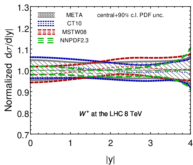
In a follow-up paper, we demonstrate that the META PDF approach performs as well for various differential observables that we explored. The META PDFs provide an average of three input PDF ensembles for various distributions, such as NNLO rapidity distributions of W and Z bosons produced at the LHC in Fig. 24, obtained with Vrap [42] at the NNLO. The rapidity distributions are normalized to the central predictions of the META PDFs, the bands indicate 90% c.l. PDF uncertainties. The central predictions of the META PDFs represent the average of the three global sets across a wide rapidity range. The META uncertainties cover the spread of the input PDF ensembles.


V Summary
Faithful estimation of the PDF dependence in theoretical predictions is relevant practically and challenging conceptually. Diversity of PDF ensembles provided by several groups reflects a variety of factors impacting the PDFs in modern QCD calculations. Comparisons of PDFs deal with their miscellaneous assumptions and disparate formats, as well as with large numbers of member sets included in the PDF ensembles. To estimate the net uncertainty in QCD cross sections due to the PDF inputs, theoretical predictions are currently calculated on a process-by-process basis for multiple PDF sets and combined at the final stage based on a certain prescription, e.g., the PDF4LHC recommendation [27, 28, 16] or the replica combination method [29, 30]. These approaches, while providing a reasonable uncertainty estimate, handle the PDFs inefficiently and promote lengthy computations. Much of the information contained in the input PDF sets is discarded in the final combination. Development of fast interpolation interfaces for (N)NLO cross sections, such as ApplGrid [63] or FastNLO [64, 51], speeds up the computation, but does not eliminate the key hurdle of inefficient information processing, especially when simulations involve many scattering processes.
The meta-analysis described in this study follows an alternative approach in which a variety of PDFs are combined into a single PDF ensemble before the individual theoretical predictions are computed. Such ensemble is suitable for most LHC applications and consists of a relatively small number of error PDFs that reproduce the total PDF+ uncertainty provided by an arbitrary number of the input PDF ensembles. In the specific example that we constructed, a META ensemble is comprised of 100 Hessian eigenvector sets for evaluating the 68% c.l. combined uncertainty of CT10, MSTW’2008, and NNPDF2.3 at NNLO. The three ensembles are selected because they can be combined with minimal obstacles. They correspond to close values of the QCD coupling strength (compatible with the world average of 0.118) and, although they follow different heavy-quark schemes, these differences can be absorbed into their parametrizations at the initial evolution scale of META PDFs chosen to be above the quark mass (at 8 GeV).
Each error set of the input ensembles is approximated by an auxiliary functional form (a meta-parametrization) in the kinematic range typical for LHC studies, taken to be and GeV. As the meta-parametrizations of all error sets share the same functional form, distributions of their free parameters (66 in total) can be easily compared. We determine these parameters at a common coupling of 0.118. Small differences in the input values are compensated for by minor shifts of the respective meta-parameters found using the series of the input PDF sets.
Then we combine the meta ensembles from CT10, MSTW2008 and NNPDF2.3 by generating Monte-Carlo replicas for each Hessian input ensemble and diagonalizing the covariance matrix constructed from the Monte-Carlo replicas. The final result consists of a central META PDF set, equivalent to the unweighted average of three input central sets, and 100 eigenvector META sets obtained in the Hessian method [12, 13]. The PDF uncertainty for the META ensemble is computed according to the master formulas in Eq. (22). We also provide a PDF series of the META PDFs for calculating the PDF+ uncertainty, including the correlations, by adding the PDF and uncertainties in quadrature [56]. The META PDFs are stored in a tabulated format together with an interface for their numerical interpolation at [37].
The META ensemble predicts about the same PDF+ uncertainty in the key LHC observables as the PDF4LHC recommendation, and in addition provides a natural way to estimate correlations of different observables. In comparison to massive computation efforts characteristic of LHC simulations, the construction of the META ensemble is relatively simple and was carried out entirely by using standard functions for statistics and data analysis in Mathematica 8.
Our results present an initial attempt to combine LHC predictions from different PDF groups independently of the processes studied. We note several avenues for further developments of this approach. The simple combination procedure that was tried (equivalent to using an unweighted average for finding expectation values) would be inappropriate for including too disparate PDF ensembles or for non-Gaussian parameter distributions. In our case, the three global ensembles that were combined are similar in their fitted experimental samples, , central PDFs, and nominal PDF uncertainties. We also examined the meta-parametrizations for ABM’11 and HERAPDF1.5 ensembles and observed that their central PDF sets for sometimes lie outside of the 90% c.l. error bands of the META ensemble, see Figs. 16 and 17. We could not fully consider the ABM’11 error sets in the current combination at a fixed , as in the ABM error sets varies around a low central value of . For HERAPDF1.5, a part of the difference with the global sets can be attributed to a larger PDF uncertainty on some combinations of the HERA PDF parameters, given their smaller experimental data set. Such an ensemble could be added by averaging the META parameters with statistical weights that account for different sizes of the experimental data samples.
The error PDFs of the future META ensembles can be obtained using either the Monte Carlo (MC) sampling or Hessian methods. In the MC approach [29, 30], probability distributions of arbitrary complexity can be in principle described, while selection of replicas is simplified via using a shared meta-parametrization form. Constraints from new experiments can be imposed using the PDF reweighting technique [14, 65, 66] in either MC or Hessian approaches. The method of data set diagonalization [54] can be applied in the case of the Hessian representation to find a small number of eigenvector sets that dominate the PDF uncertainty of given observables. While the 100 META eigenvector sets are designated for a wide range of LHC theoretical predictions, a much smaller number (6-10) of eigenvector sets dominates the uncertainty in various important processes, such as massive electroweak boson production [55]. The framework of the meta-analysis is well-suited for exploring these possibilities.
ACKNOWLEDGMENTS
This work was supported by the U.S. DOE Early Career Research Award DE-SC0003870 and by Lightner-Sams Foundation. We appreciate insightful discussions with Sayipjamal Dulat, Joey Houston, Jon Pumplin, Carl Schmidt, Dan Stump, Robert Thorne, Graeme Watt, and C.-P. Yuan.
References
- [1] G. Aad et al. (ATLAS Collaboration), Phys.Lett. B716, 1 (2012a), eprint 1207.7214.
- [2] S. Chatrchyan et al. (CMS Collaboration), Phys.Lett. B716, 30 (2012a), eprint 1207.7235.
- [3]
Higgs Working Group Report, Snowmass’2013 Community Planning
study,
http://www.snowmass2013.org/tiki-index.php?page=The+Higgs+Boson. - [4] J. Gao, M. Guzzi, J. Huston, H.-L. Lai, Z. Li, et al., Phys.Rev. D89, 033009 (2014), eprint 1302.6246.
- [5] A. Martin, W. Stirling, R. Thorne, and G. Watt, Eur.Phys.J. C63, 189 (2009a), eprint 0901.0002.
- [6] R. D. Ball, V. Bertone, S. Carrazza, C. S. Deans, L. Del Debbio, et al., Nucl.Phys. B867, 244 (2013a), eprint 1207.1303.
- [7] S. Alekhin, J. Blumlein, and S. Moch, Phys.Rev. D86, 054009 (2012), eprint 1202.2281.
- [8] S. Alekhin, J. Bluemlein, and S. Moch (2013), eprint 1310.3059.
- [9] P. Jimenez-Delgado and E. Reya, Phys.Rev. D79, 074023 (2009a), eprint 0810.4274.
- [10] P. Jimenez-Delgado and E. Reya, Phys.Rev. D80, 114011 (2009b), eprint 0909.1711.
- [11] A. Cooper-Sarkar (ZEUS Collaboration, H1 Collaboration), PoS EPS-HEP2011, 320 (2011), eprint 1112.2107.
- [12] J. Pumplin, D. Stump, R. Brock, D. Casey, J. Huston, et al., Phys.Rev. D65, 014013 (2001), eprint hep-ph/0101032.
- [13] J. Pumplin, D. Stump, J. Huston, H. Lai, P. M. Nadolsky, et al., JHEP 0207, 012 (2002), eprint hep-ph/0201195.
- [14] W. T. Giele and S. Keller, Phys.Rev. D58, 094023 (1998), eprint hep-ph/9803393.
- [15] L. Del Debbio, S. Forte, J. I. Latorre, A. Piccione, and J. Rojo (NNPDF Collaboration), JHEP 0703, 039 (2007), eprint hep-ph/0701127.
- [16] R. D. Ball, S. Carrazza, L. Del Debbio, S. Forte, J. Gao, et al., JHEP 1304, 125 (2013b), eprint 1211.5142.
- [17] J. Owens, A. Accardi, and W. Melnitchouk, Phys.Rev. D87, 094012 (2013), eprint 1212.1702.
- [18] J. Pumplin, H. Lai, and W. Tung, Phys.Rev. D75, 054029 (2007), eprint hep-ph/0701220.
- [19] S. Dulat, T.-J. Hou, J. Gao, J. Huston, J. Pumplin, et al. (2013), eprint 1309.0025.
- [20] A. Martin, R. Roberts, W. Stirling, and R. Thorne, Eur.Phys.J. C39, 155 (2005), eprint hep-ph/0411040.
- [21] R. D. Ball et al. (NNPDF), Nucl.Phys. B877, 290 (2013c), eprint 1308.0598.
- [22] E. Askanazi, K. Holcomb, and S. Liuti (2013), eprint 1309.7085.
- [23] K. Kovarik, T. Jezo, A. Kusina, F. Olness, I. Schienbein, et al., PoS DIS2013, 274 (2013), eprint 1307.3454.
- [24] M. Hirai, S. Kumano, and T.-H. Nagai, Phys.Rev. C76, 065207 (2007), eprint 0709.3038.
- [25] K. Eskola, H. Paukkunen, and C. Salgado, JHEP 0904, 065 (2009), eprint 0902.4154.
- [26] D. de Florian, R. Sassot, P. Zurita, and M. Stratmann, Phys.Rev. D85, 074028 (2012), eprint 1112.6324.
- [27] M. Botje, J. Butterworth, A. Cooper-Sarkar, A. de Roeck, J. Feltesse, et al. (2011), eprint 1101.0538.
- [28] S. Alekhin, S. Alioli, R. D. Ball, V. Bertone, J. Blumlein, et al. (2011), eprint 1101.0536.
- [29] S. Forte and G. Watt, Ann.Rev.Nucl.Part.Sci. 63, 291 (2013), eprint 1301.6754.
- [30] S. Forte, Acta Phys.Polon. B41, 2859 (2010), eprint 1011.5247.
- [31] J. Beringer et al. (Particle Data Group), Phys.Rev. D86, 010001 (2012).
- [32] P. M. Nadolsky and Z. Sullivan, eConf C010630, P510 (2001), eprint hep-ph/0110378.
- [33] P. M. Nadolsky, H.-L. Lai, Q.-H. Cao, J. Huston, J. Pumplin, et al., Phys.Rev. D78, 013004 (2008), eprint 0802.0007.
- [34] J. Pumplin, Phys.Rev. D82, 114020 (2010), eprint 0909.5176.
- [35] A. Glazov, S. Moch, and V. Radescu, Phys.Lett. B695, 238 (2011), eprint 1009.6170.
- [36] A. Martin, A. T. Mathijssen, W. Stirling, R. Thorne, B. Watt, et al., Eur.Phys.J. C73, 2318 (2013), eprint 1211.1215.
- [37] http://metapdf.hepforge.org/.
- [38] S. Moch, J. Vermaseren, and A. Vogt, Nucl.Phys. B688, 101 (2004), eprint hep-ph/0403192.
- [39] A. Vogt, S. Moch, and J. Vermaseren, Nucl.Phys. B691, 129 (2004), eprint hep-ph/0404111.
- [40] http://lhapdf.hepforge.org/.
- [41] G. P. Salam and J. Rojo, Comput.Phys.Commun. 180, 120 (2009), eprint 0804.3755.
- [42] C. Anastasiou, L. J. Dixon, K. Melnikov, and F. Petriello, Phys.Rev. D69, 094008 (2004), eprint hep-ph/0312266.
- [43] C. Anastasiou, S. Buehler, F. Herzog, and A. Lazopoulos, JHEP 1112, 058 (2011), eprint 1107.0683.
- [44] P. Bärnreuther, M. Czakon, and A. Mitov, Phys.Rev.Lett. 109, 132001 (2012), eprint 1204.5201.
- [45] M. Czakon and A. Mitov, JHEP 1212, 054 (2012), eprint 1207.0236.
- [46] M. Czakon and A. Mitov, JHEP 1301, 080 (2013), eprint 1210.6832.
- [47] M. Czakon and A. Mitov (2011), eprint 1112.5675.
- [48] M. Beneke, P. Falgari, and C. Schwinn, Nucl.Phys. B828, 69 (2010), eprint 0907.1443.
- [49] M. Czakon, A. Mitov, and G. F. Sterman, Phys.Rev. D80, 074017 (2009), eprint 0907.1790.
- [50] M. Cacciari, M. Czakon, M. Mangano, A. Mitov, and P. Nason, Phys.Lett. B710, 612 (2012), eprint 1111.5869.
- [51] M. Wobisch, D. Britzger, T. Kluge, K. Rabbertz, and F. Stober (fastNLO Collaboration) (2011), eprint 1109.1310.
- [52] G. Aad et al. (ATLAS Collaboration), Phys.Rev. D86, 014022 (2012b), eprint 1112.6297.
- [53] G. Watt and R. Thorne, JHEP 1208, 052 (2012), eprint 1205.4024.
- [54] J. Pumplin, J. Huston, H. Lai, P. Nadolsky, W.-K. Tung, et al., Phys.Rev. D80, 014019 (2009), eprint 0904.2424.
- [55] J. Gao, J. Huston, and P. M. Nadolsky, in preparation.
- [56] H.-L. Lai, J. Huston, Z. Li, P. Nadolsky, J. Pumplin, et al., Phys.Rev. D82, 054021 (2010), eprint 1004.4624.
- [57] A. Martin, W. Stirling, R. Thorne, and G. Watt, Eur.Phys.J. C64, 653 (2009b), eprint 0905.3531.
- [58] R. D. Ball, V. Bertone, L. Del Debbio, S. Forte, A. Guffanti, et al., Phys.Lett. B707, 66 (2012), eprint 1110.2483.
- [59] G. Aad et al. (ATLAS Collaboration), Phys.Rev. D85, 072004 (2012c), eprint 1109.5141.
- [60] R. Aaij et al. (LHCb Collaboration), JHEP 1206, 058 (2012), eprint 1204.1620.
- [61] S. Chatrchyan et al. (CMS Collaboration), Phys.Rev.Lett. 109, 111806 (2012b), eprint 1206.2598.
- [62] J. M. Campbell, J. Huston, and W. Stirling, Rept.Prog.Phys. 70, 89 (2007), eprint hep-ph/0611148.
- [63] M. Sutton, T. Carli, D. Clements, A. Cooper-Sarkar, C. Gwenlan, et al., PoS DIS2010, 051 (2010).
- [64] T. Kluge, K. Rabbertz, and M. Wobisch, pp. 483–486 (2006), eprint hep-ph/0609285.
- [65] R. D. Ball et al. (NNPDF Collaboration), Nucl.Phys. B849, 112 (2011), eprint 1012.0836.
- [66] N. Sato, J. Owens, and H. Prosper (2013), eprint 1310.1089.
Appendix. A test of QCD evolution
In this appendix, we verify that the dependence of and PDFs on the scale in the input ensembles is compatible and allows their combination. We compared the tabulated evolution of and for five ensembles from the LHAPDF library [40] with the numerical evolution by the HOPPET program [41] from the initial scale GeV up to GeV. In all cases, we assume 3 QCD loops and 5 flavors in the QCD beta-function and splitting kernels.
Fig. 25 shows the ratio of that we get from LHAPDF to the corresponding values from HOPPET using the original values of the input ensembles listed in Table 1. The agreement of the tabulated and evolved is perfect for all ensembles except for HERAPDF, where a kink at the top quark mass occurs because HERAPDF uses the 6-flavor above the top quark threshold.
The PDF evolution is examined by computing ratios of returned by LHAPDF and HOPPET at several values above 8 GeV. The -dependent ratios at 0 GeV shown in Fig. 26 are representative of the general trend at other values. We observe excellent agreement at the level of 0.1% between LHAPDF and HOPPET for both CT10 and NNPDF almost across the entire shown region of , except for , where differences in the dependence can be a few percent for all sea PDFs. In the case of ABM, fluctuations for all sea PDFs are observed at somewhat smaller values of of about 0.3, but again they happen in the region where the sea PDFs are small, and the accuracy of LHAPDF interpolation is sufficient compared to the PDF uncertainties. The tabulated and numerical evolution of quark PDFs from MSTW shows a systematic discrepancy reaching 1% at , while the tabulated and numerical evolution of the MSTW gluon is in a perfect agreement. The tabulated and evolved HERA PDFs differ by across most , which is expected at GeV given the 5-flavor evolution in HOPPET and 6-flavor evolution of the HERAPDF’s tabulated .


