Sideband generation of transient lasing without population inversion

Introduction. — As a fundamental aspect of nonlinear optics, optical sidebands generated via frequency modulation, attracts widespread interest and have versatile applications in atomic systems [1, 2, 3], terahertz quantum cascade lasers [4], ultrafast driven optomechanical systems [5], polymer waveguides on a printed circuit [6], and so on [7, 8]. In these cases, a probe laser source is needed and optical sidebands are produced by the interaction between the probe laser and the modulated medium. However, the addition of this extra probe laser not only increases the complexity of the experiment, but also introduces a limit to this technology because it is difficult to prepare a table-top laser pulse in some specific frequency regimes, i.e. in the extreme ultraviolet (XUV) or x-ray regime and the THz regime.

Lasing without inversion (LWI) [9, 10, 11, 12] has been studied in various media, such as in gas [13], circuit quantum electrodynamics [14], and terahertz intersubband-based devices [15]. By preparing an atomic system in a coherent superposition of states it is possible to create atomic coherence to suppress absorption resulting in LWI [16]. Steady-state LWI requires that the spontaneous decay rate of the pumping transition is larger than the decay rate of the lasing transition [17], which is difficult to achieve when the frequency of the lasing transition is higher than the drive field frequency. Thanks to a recent experiment showing that a large collective atomic coherence can be built up during a superradiant time scale much shorter than the collisional decoherence time [18], these obstacles can be overcome in LWI in the transient regime [12], where the lasing happens at a much shorter time than the decoherence time and therefore all the decay rates can be neglected. This paves the way for more complicated manipulation of the quantum coherence to achieve sideband lasing at multiple frequencies without initial population inversion.

In this letter, we combine the concepts of transient LWI and of sideband generation to realize frequency comb generation at high frequencies. The transient LWI is explored in a more complete picture than any previous works by considering all the frequency mode components. Through making a single-pass superradiant gain [19, 20], our results provide a new route toward generating multiple-frequency coherent light and have implications for the ultrashort pulse creation, short-wavelength coherent light sources in the XUV and X-ray regime, and tunable THz laser generation.

Model. — The mechanism of our proposal is shown in Fig. 1 (Left) based on a three-level V-type system. The system is initially prepared such that most of the population remains in the ground state but a little population is in the excited state $|a\rangle$. A strong driving field $\Omega^{\text{drive}}$ propagates into the pencil-like active medium and couples the transition $c\leftrightarrow b$. A Floquet ladder [21] is generated (see Fig. 1 (Right)). The transitions from $a$ to the Floquet ladder produce various lasing fields with frequency $\nu_{l}\sim\omega_{ab}+2j\nu_{d}$ ($j=0,\pm 1,\pm 2,\dots$) in a time scale much shorter than any decay time. Here $\nu_{l}$ is the lasing frequency, $\omega_{ab}$ is the atomic transition, $\nu_{d}$ is the driving field frequency. These fields are coupled by $\Omega^{\text{drive}}$ via the atomic coherence. The frequency difference between sidebands is always an even multiple of $\nu_{d}$ since an atom in state $|i\rangle$ needs an even number of photons to return to its original state $|i\rangle$, through successive real and virtual processes (where the counter-rotating terms play a role) [22, 23].

The simple but important physics behind the frequency comb gain profile can be understood by considering the dressed-state picture. By driving the $c\rightarrow b$ transition, the excited state $a$ is coupled with two dressed states ($j^{+}$, $j^{-}$) at each order in the Floquet ladder (see Fig. 1). Both of the allowed transition frequencies are on the order of $\omega_{ab}+2j\nu_{d}$. The energy difference between two dressed states depends on the drive field Rabi frequency $\Omega_{d}$ and the drive field detuning $\Delta$. The initial population in the ground state $b$ is redistributed to the two split dressed states at each order. While there is no population inversion in the bare-state system, it is still possible to achieve transient lasing because of the population inversion in dressed-state picture. Through the coupled atomic coherence, different sideband modes are consequently amplified. The lasing threshold can be reached by tuning the driving field intensity and the medium length.

To start our analysis, we assume that $\rho_{bb}$, $\rho_{cc}$, and $\rho_{cb}$ evolve only under the influence of the driving field for the moment (see the corresponding equations in the Appendix A) because the laser field coupled with $a\leftrightarrow b$ transition is relatively weak. The drive field $\Omega^{\mathrm{drive}}=\Omega_{d}\cos[\nu_{d}(t-z/c)]$ is turned on adiabatically. We look for the solutions in the forms $\rho_{bc}(t,z)=\sum_{m}\rho_{bc}^{m}e^{-im\nu_{d}(t-z/c)}$, $\rho_{bb}(t,z)=\sum_{m}\rho_{bb}^{m}e^{-im\nu_{d}(t-z/c)}$. A set of infinite coupled algebraic equations can be derived and the solutions for $\rho_{bc}^{m}$ and $\rho_{bb}^{m}$ are found numerically. The detail is in the Appendix B.

The propagation of the laser pulse is described by Maxwell’s equation [16]

where $\Omega_{a}\equiv\sqrt{\frac{3N\lambda_{ab}^{2}\gamma c}{8\pi}}$, where $N$ is the density, $\lambda_{ab}$ is the $a\rightarrow b$ transition wavelength, $\gamma$ is the $a\rightarrow b$ radiative decay rate, and $c$ is the speed of light. The atomic coherences $\rho_{ab}$ and $\rho_{ac}$ evolve with Eqs. (A-1) and (A-2) in the Appendix A. We are looking for a solution in the form of a superposition of spectral components without the rotating-wave-approximation (RWA) [1],

where $m=0,\pm 1,\pm 2,\ldots$, and $\Delta\nu$ is the small detuning of the lasing frequency from the frequency $\omega_{ab}+m\nu_{d}$. By using the expressions in Eqs. (2)-(4) and taking the components for the same frequency mode $m$ with slowly-varying-envelope approximation (SVEA), the equations of the evolution of the laser field becomes

where $\omega_{m}\equiv\omega_{ab}+m\nu_{d}+\Delta\nu$. Here introduce next set of coupled algebraic equations which combine the equations that describe the evolution of the coherence $\rho_{ab}$ and $\rho_{ac}$

where we define $\eta_{m}^{\pm}\equiv 1/\left(\omega_{cb}\pm\nu_{d}+m\nu_{d}+\Delta\nu+i\gamma_{t}\right)$, $\Phi_{m}^{\pm}\equiv-\Omega_{d}^{2}\eta_{m}^{\pm}/4$, $\Phi_{m}^{0}\equiv\left(m\nu_{d}+\Delta\nu+i\gamma_{t}\right)-\Omega_{d}^{2}\left(\eta_{m}^{-}+\eta_{m}^{+}\right)/4$, and $\Theta_{m}^{2q}\equiv\rho_{bb}^{2q}-\rho_{aa}(0)\delta_{q0}+\Omega_{d}\left(\eta_{m}^{-}\rho_{bc}^{2q-1}+\eta_{m}^{+}\rho_{bc}^{2q+1}\right)/2$, where $\gamma_{t}$ is the total decoherence rate, which is negligible in the transient regime. Eq. (6) indicates that the component of the field at the mode $m$ is coupled with those at modes $m+2j$, where j is the integer.

We search for a solution of Eq. (6) with the form,

Using this form in Eq. (5), we obtain $\rho_{ab}^{m}(z)=\frac{\omega_{ab}}{\omega_{ab}+m\nu_{d}+\Delta\nu}\frac{c}{\Omega_{a}^{2}}\sum_{n}u_{n}\varepsilon_{n}^{m}k_{n}e^{ik_{n}z}$. With the trial solutions of $\Omega_{l}^{m}$ and $\rho_{ab}^{m}$, Eq. (6) results in an infinite set of linear equations with eigenvalues $k_{n}$ and their corresponding eigenvectors $\hat{\varepsilon}_{n}=\left(\dots,\varepsilon_{n}^{m-2},\varepsilon_{n}^{m},\varepsilon_{n}^{m+2},\dots\right)^{T}$. The coefficient $u_{n}$ is determined by the boundary conditions for $\Omega_{l}^{m}(z=0)$ and it reads $u_{n}=\sum_{m}\varepsilon_{n}^{m}\Omega_{l}^{m}(z=0)$. There are an infinite coupled number of frequency modes. However, the spectra must have a central spectral region where all the frequency modes have relatively strong intensities while the other frequencies far away from this region fade out gradually. Therefore, we can solve Eq. (6) numerically in a central spectral region where it has central mode $m=0$ and boundary modes $m=m_{0}$. The set of infinite equations is truncated to dimension $(m_{0}+1)\times(m_{0}+1)$ [22].

We first show the basic result in Fig. 2. The gain is characterized by the imaginary parts of eigenvalues $k_{n}$ ($n=$1, 2,… with descending magnitudes of their imaginary parts) of Eq. (6), since the fields generally follow $\sim e^{-\text{Im}k_{1}z}$. Especially, we focus on the leading eigenvalue $k_{1}$ whose imaginary part has a magnitude several orders larger than the rest. A peak of $-\mathrm{Im}(k_{1})$ appears at $\Delta\nu\sim 1.05\Delta$ with width $\sim 0.01\Delta$ where $\Delta\equiv\nu_{d}-\omega_{cb}$. We therefore can observe sideband LWI in this region.

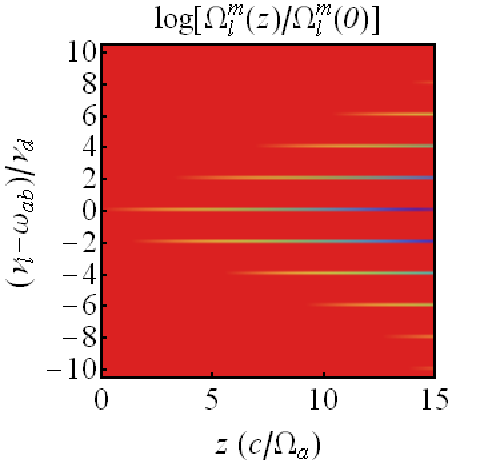
The amplitude of the output field at frequency mode $m$ ($\Omega_{l}^{m}$) is determined by Eq. (7). The gain of each frequency component is not only dependent on the imaginary part of the eigenvalues, but also dependent on the coefficients such as $\varepsilon_{n}^{m}$, the elements in the eigenstates and $u_{n}$ due to the boundary condition. It results in different lasing amplifications for different frequency modes. If the field component has smaller coefficients, it requires a longer propagation length to be amplified. The result is plotted in Fig. 3. We find that we generate a frequency comb at a long propagation distance ($z=15$ ($c/\Omega_{a}$)). With longer propagation length, sideband lasing at the higher-order modes gets amplified. For the field at mode $m\neq 0$ ($\Omega_{l}^{m}(z)$) with frequency $\sim\omega_{ab}+m\nu_{d}$, the component of $k_{1}$ in Eq. (7) does not dominate over the components of the other eigenvalues for small $z$, so the field component $\Omega_{l}^{m}(z)$ is not amplified compared to its initial value ($\Omega_{l}^{m}(0)$). This means that the laser field has threshold behavior and the one at a larger frequency mode has a higher threshold value (see Fig. 3). The amplification quantity $\log[\Omega_{l}^{m}(L)/\Omega_{l}^{m}(0)]$ is linearly dependent on the propagation length $L$ only if the propagation length $L$ exceeds the threshold value. In this regime, the linear coefficients for each curve at different frequency modes are the same because the leading terms in Eq. (7) for all modes $m$ are the components of $k_{1}$ for large $z$ and all those terms grow according to $\exp(-\mathrm{Im}k_{1}z)$.

The amplification of the laser pulse in the whole spectral region has a common source $-\mathrm{Im}(k_{1})$. We study the relation between $k_{1}$ and the drive field Rabi frequency $\Omega_{d}$ with all the other parameters fixed. We solve Eq. (6) numerically for various $\Omega_{d}$ and search the maximum value of $-\mathrm{Im}(k_{1})_{\mathrm{max}}$, by scanning the lasing frequency detuning $\Delta\nu$ for each set of parameters. The dependence of the quantity $-\mathrm{Im}(k_{1})_{\mathrm{max}}$ with its corresponding lasing frequency detuning $\Delta\nu$ on different $\Omega_{d}$ are plotted in Fig. 4. All of the other parameters are the same as in Fig. 2. We find that the quantity $-\mathrm{Im}(k_{1})_{\mathrm{max}}$ is increasing with the drive field Rabi frequency $\Omega_{d}$ when $\Omega_{d}$ is small. Nevertheless $-\mathrm{Im}(k_{1})_{\mathrm{max}}$ has a maximum after which it drops counter-intuitively with increasing $\Omega_{d}$.

This behavior can be explained in the dressed-state picture. Each order of the Floquet ladder of states is split in two dressed states (as shown in Fig. 1). If $\Omega_{d}\rightarrow 0$, one of the two dressed states (level $2j^{-}$ in the current case) has $\sim 0$ population, but the corresponding coupling strength between this dressed state and the excited state also goes to zero. The increase of $\Omega_{d}$ leads to the enhancement of this coupling strength and results in the increase of the gain. However, larger $\Omega_{d}$ also leads to more population in this dressed state, resulting in less population inversion. The competition between these two mechanisms is the reason that the quantity $-\mathrm{Im}(k_{1})_{\mathrm{max}}$ has the maximum positive value when $\Omega_{d}$ is near the resonance $\sim 0.1\omega_{cb}$ (see Fig. 4). Only one of the two split dressed states ($2j^{-}$) can have less population than the excited state, so there is only one peak of the imaginary part of the eigenvalue $k_{1}$ as shown in Fig. 2. (This is summarized in the detailed derivation in the Appendix C.) On the other hand, changing the drive field Rabi frequency modifies the energies of the two dressed states, so the corresponding lasing frequency detuning $\Delta\nu$ is increasing versus $\Omega_{d}$ (right purple curve in Fig. 4).

The generated frequency comb has many applications:

Ultrashort pulse generation. — Ultrashort pulse production can be achieved by modifying an input single-frequency field to create an output field with multi-frequencies at the same phase [1, 24, 25]. In contrast our method is valid for generating the ultrashort pulse without the requirement of an input field at the same centered frequency as the desired output pulse. A low-frequency drive is used to modulate the system. We choose Hydrogen molecule as an example, which has its first vibrational transition frequency at the ground electronic state $\lambda_{cb}=2.28$ $\mu$m and a high-frequency electronic transition ($B$ ${}^{1}\Sigma_{u}^{+}$ $\leftrightarrow$ $X$ ${}^{1}\Sigma_{g}^{+}$) at the frequency $\lambda_{ab}=109$ nm. Few-cycle pulse with 5 fs linewidth and 22 fs repetition period is produced by converting the central 5 sideband LWIs at different spectral components attenuated to equal values with frequency-resolved filters (see Fig. 5). The physical mechanism is similar to Ref. [1]. By changing to a different active medium, it is possible to further shorten the pulse width.

Short-wavelength laser. — The conversion from the long-wavelength drive pulse to the short-wavelength emission pulse, in particular the pulses at the blue-shifted sidebands ($m>0$), provides a promising choice for generating a high-frequency laser. Consider as a proof-of-principle, the realistic experimental choice of a helium plasma gas which is partially excited to the metastable triplet state, 2 ${}^{3}\mathrm{S}_{1}$, as realized in one recent experiment [18]. Where the density is $\sim 10^{16}$ cm^-3 and we can drive the infrared transition 2 ${}^{3}\mathrm{P}_{1}\rightarrow$2 ${}^{3}\mathrm{S}_{1}$ (1083 nm) with a drive field wavelength as $\lambda_{d}=1022$ nm and a Rabi frequency of $\Omega_{d}\sim 10^{14}$ rad/s. The dispersion of the drive field is negligible if it is detuned significantly from the resonance. A little population is left in the excited state 3 ${}^{3}\mathrm{P}_{1}$ by non-radiative three-body recombination following an optical field ionization. This allows transient LWI to occur at the ultraviolet transition 3 ${}^{3}\mathrm{P}_{1}\rightarrow$2 ${}^{3}\mathrm{S}_{1}$ (388.9 nm). The higher-order sideband lasing would have wavelengths as $\lambda_{l}^{(2)}\sim 220.8$ nm, $\lambda_{l}^{(4)}\sim 154.2$ nm, etc. In a 1-cm long medium, we find a single-pass nano-Joule level coherent emission at the wavelength $\sim 220.8$ nm with the parameters listed above. In principle, this method can make table-top laser pulses in XUV and X-ray regime with a visible driving field.

Tunable THz laser. — Graphene has suitable energy level structure with strong dipole moments to study the physics in the THz regime in a magnetic field [26, 27]. The V-scheme model is composed of the Landau levels (LLs) near the Dirac point with energy quantum numbers -2, -1, and 3. $B\sim 1.4$ mT gives the transition frequency $\omega_{cb}/2\pi\sim 140$ GHz between LLs with energy quantum numbers -2 and -1, which can be driven by commercially available facilities for coherent millimeter wave source. Propagation effects are complicated by the large number of graphene layers [28]; our model shows sideband LWI at frequencies $1.06\pm 0.28n$ THz ($n=0,1,2,\ldots$). The transition frequencies in the V-scheme can be further changed by modifying the magnetic field. The emission at different frequencies in THz regime can be used to build a tunable THz laser.

In conclusion, we study Frequency comb generation via sideband transient LWI. We use the Floquet method to solve the system in the weak lasing field limit (the population is unchanged due to the lasing field) and find amplified emission at different frequency modes. Threshold behavior is seen for high-order sidebands. This universal model has many possible applications including ultrashort pulse generation, short-wavelength laser in the XUV and X-ray regime, and tunable THz laser source. We gave an example scheme for the generation of 5-fs pulses in molecular hydrogen.

References

- [1] Y.V. Radeonychev, V.A. Polovinkin, and O. Kocharovskaya, Phys. Rev. Lett. 105, 183902 (2010).
- [2] A.M. Akulshin, R.J. McLean, A.I. Sidorov, and P. Hannaford, J. Phys. B: At. Mol. Opt. Phys. 44, 175502 (2011).
- [3] S. M. Cavaletto, Z. Harman, C. Ott, C. Buth, T. Pfeifer, and C. H. Keitel, Nat. Photonics DOI: 10.1038/NPHOTON.2014.113.
- [4] P. Cavalié, J. Freeman, K. Maussang, E. Strupiechonski, G. Xu, R. Colombelli, L. Li, A.G. Davies, E.H. Linfield, J. Tignon, and S.S. Dhillon, Appl. Phys. Lett. 102, 221101 (2013).
- [5] H. Xiong, L.-G. Si, X.-Y. Lü, X. Yang, and Y. Wu, Opt. Lett. 38, 353 (2013).
- [6] A.A. Lanin, I.V. Fedotov, V.I. Sokolov, A.B. Fedotov, A.S. Akhmanov, V.Ya. Panchenko, and A.M. Zheltikov, Opt. Lett. 35, 3976 (2010).
- [7] A. Schliesser, R. Rivière, G. Anetsberger, O. Arcizet, and T.J. Kippenberg, Nat. Phys. 4, 415 (2008).
- [8] S.N. Soda, S. Sensarn, M.Y. Shverdin, and G.Y. Yin, Appl. Phys. Lett. 91, 241101 (2007).
- [9] O.A. Kocharovskaya and Ya.I. Khanin, JETP Lett. 48, 630 (1988).
- [10] S.E. Harris, Phys. Rev. Lett. 62, 1033 (1989).
- [11] M.O. Scully, S.-Y. Zhu, and A. Gavrielides, Phys. Rev. Lett. 62, 2813 (1989).
- [12] A.A. Svidzinsky, L. Yuan, and M.O. Scully, New J. Phys. 15, 053044 (2013).
- [13] E.S. Fry, X. Li, D. Nikonov, G.G. Padmabandu, M.O. Scully, A.V. Smith, F.K. Tittel, C. Wang, S.R. Wilkinson, and S.-Y. Zhu, Phys. Rev. Lett. 70, 3235 (1993).
- [14] M. Marthaler, Y. Utsumi, D.S. Golubev, A. Shnirman, and G. Schön, Phys. Rev. Lett. 107, 093901 (2011).
- [15] M.F. Pereira, Jr. Phys. Rev. B 78, 245305 (2008).
- [16] M.O. Scully and M.S. Zubairy, Quantum Optics (Cambridge University Press, New York, NY 1997).
- [17] A. Imamoglu, J. E. Field, and S. E. Harris, Phys. Rev. Lett. 66, 1154 (1991).
- [18] H. Xia, A.A. Svidzinsky, L. Yuan, C. Lu, S. Suckewer, and M.O. Scully, Phys. Rev. Lett. 109, 093604 (2012).
- [19] A.E. Siegman, lasers (University Science Books, Sausalito, CA 1986).
- [20] A.A. Svidzinsky, L. Yuan, and M.O. Scully, Phys. Rev. X 3, 041001 (2013).
- [21] G.N. Gibson, Phys. Rev. Lett. 89, 263001 (2002).
- [22] A. Picón, L. Roso, J. Mompart, O. Varela, V. Ahufinger, R. Corbalán, and L. Plaja, Phys. Rev. A 81, 033420 (2010).
- [23] D.-w. Wang, A.-j. Li, L.-g. Wang, S.-y. Zhu, and M.S. Zubairy, Phys. Rev. A 80, 063826 (2009).
- [24] S.E. Harris and A.V. Sokolov, Phys. Rev. Lett. 81, 2894 (1998).
- [25] M. Zhi, K. Wang, X. Hua, and A.V. Sokolov, Opt. Lett. 36, 4032 (2011).
- [26] X. Yao and A. Belyanin, Phys. Rev. Lett. 108, 255503 (2012).
- [27] M. Tokman, X. Yao, and A. Belyanin, Phys. Rev. Lett. 110, 077404 (2013).
- [28] N. Jung, A.C. Crowther, N. Kim, P. Kim, and L. Brus, ACS Nano 4, 7005 (2010).
- [29] J.C. MacGillivray and M.S. Feld, Phys. Rev. A 14, 1169 (1976).