Highly Dispersed Networks Generated by Enhanced Redirection

Macrohubs always arise when $\lambda>0$, but they are easily detectable only when the exponent $\nu$ is notably smaller than 2. Figure 4 shows that this happens when $\lambda\mathrel{\raise 2.58334pt\hbox{$>$\kern-7.5pt\lower 5.16663pt\hbox{$\sim$}}}0.4$, and in this range macrohubs are clearly observed in all network realizations. When the redirection parameter is small, $0<\lambda<0.4$, it may be necessary to grow the network to an astronomically large value of $N$ to detect macrohubs with certainty.

There are usually many macrohubs, whose degree is proportional to $N$, as shown in Fig. 6(a). To estimate $k_{m}$, the degree of the $m^{\text{th}}$ largest macrohub, we use the extremal criterion [31],

This equation merely states that there should be of the order of $m$ nodes of degree $k_{m}$ or larger. Thus $k_{m}$ indeed gives an estimate for the value of the $m^{\rm th}$-largest degree. Combining this criterion with the asymptotic $N_{k}\sim N^{\nu-1}/k^{\nu}$ from Eq. (1) gives

The basic feature is that the degrees of macrohubs scale linearly with $N$. In contrast, for networks with an extensive degree distribution of the form $N_{k}\sim N/k^{\nu}$ and $\nu>2$, the above extremal criterion gives the sub-linear growth: $k_{m}\sim(N/m)^{1/(\nu-1)}$.

The degrees of the macrohubs substantially depends on the early stages of network growth, but once a set of macrohubs emerges (with degrees $k_{1}$, $k_{2}$, $k_{3}$, $\dots$), the probability of attaching to a macrohub of degree $k_{m}$ asymptotically approaches to $k_{m}/N$. This preferential attachment to macrohubs is similar to a Pólya urn process for filling an urn with balls of several colors [32, 33]. In the urn process, a ball is drawn at random from the urn and then replaced along with an additional matching-color ball. The different colors in the urn process correspond to different macrohubs in enhanced redirection. If there are $k_{m}$ balls of the $m^{th}$ color in an urn of $N$ total balls, then the probability of choosing color $m$, and thus increasing $k_{m}$, is given by $k_{m}/N$. For the Pólya urn process, the ultimate fractions of balls of different colors do not self-average; the same is expected for the scaled degrees of macrohubs in enhanced redirection.

Because of the tendency to link to high-degree nodes, it is possible that a star graph arises in which single node is connected to every other node of the network. As we now show, the probability for such a star to occur is non-zero for $\lambda>1$. For the initial condition of a single node with a self loop, the star contains $N-1$ leaves, while the root node has degree $N+1$. The probability $S_{N}$ to build such a star graph is

The factor $\frac{1}{n}$ accounts for the new node attaching to the root in a network of $n$ nodes, while the second term accounts for first choosing a leaf and then redirecting to the root. As shown in A, the asymptotic behavior of (13) is

where $\mathcal{S}(\lambda)=\lim_{N\to\infty}S_{N}(\lambda)$ is a monotonically increasing function of $\lambda$ when $\lambda>1$ and $A=\pi^{-1}\sinh\pi\approx 3.676$.

For $0<\lambda\leq 1$, the probability of a star graph asymptotically approaches zero as $N\to\infty$. In this range, the network typically has many macrohubs with average sizes distributed according to Eq. (12). For $\lambda>1$, a star graph occurs with a positive probability (Fig. 7), with a continuous phase transition at $\lambda=1$. As shown in A, this phase transition has an infinite order because all derivatives of $\mathcal{S}(\lambda)$ vanish at $\lambda=1$.

We now study the size distribution of the largest macrohub, the $2{{}^{\text{nd}}}$ largest macrohub, etc. By ‘size’ we mean the degree of a macrohub, so that there is no confusion between the size of the largest macrohub (a quantity characterizing one node) and the degree distribution which specifies the number of nodes of a fixed degree.

The degree $k_{m}$ of the $m^{\text{th}}$ largest macrohub scales linearly with the total number of nodes $N$, and therefore the corresponding size distribution $M_{m}(k_{m},N)$ approaches the scaling form

in the $N\to\infty$ limit. We do not know how to compute the scaling functions $\mathcal{M}_{m}(x)$, but some generic properties of these functions can be established without calculations. For instance, the scaling function $\mathcal{M}_{m}(x)$ vanishes when $x>1/m$. Indeed, the $m^{\text{th}}$-largest macrohub has maximal degree $k_{m}=N/m$, which corresponds to the situation when the first $m$ largest macrohubs all have equal maximally possible size $N/m$. Thus $\mathcal{M}_{m}(x)$ is singular at $x=1/m$: $\mathcal{M}_{m}(x)\equiv 0$ when $x>1/m$, and $\mathcal{M}_{m}(x)>0$ when $x<1/m$. Consider now the most interesting function $\mathcal{M}_{1}(x)$, which describes the scaled degree of the largest macrohub. It has a singularity at $x=1$, and also a singularity at $x=1/2$, as at this point the second-largest macrohub can emerge. Continuing this line of reasoning, we conclude that $\mathcal{M}_{1}(x)$ has infinitely many singularities that are located at $x=1,1/2,1/3,1/4,\ldots$. The emergence of these progressively weaker singularities is a generic feature and they arise in numerous examples including random walks, random maps, spin glasses, fragmentation, etc., which are characterized by the lack of self-averaging, see, e.g., [34, 35, 36, 37, 38]. Similarly, the scaling function $\mathcal{M}_{m}(x)$ has singularities at $x=1/m,1/(m+1),1/(m+2),\ldots$.

The presence of infinitely many singularities (partly) explains why it is difficult to compute the scaling functions $\mathcal{M}_{m}(x)$. Fortunately, it is possible to probe the asymptotic behavior of $\mathcal{M}_{m}(x)$ near the maximal possible size $x=1/m$. Consider the most interesting case of the largest macrohub. To determine the asymptotic behavior of $\mathcal{M}_{1}(x)$ in the $x\to 1$ limit, we notice that it can be extracted from the probability to build a star graph. Comparing (14) with (15) we find that in the marginal case of $\lambda=1$

while in the $0<\lambda<1$ range, the scaling function $\mathcal{M}_{1}(x)$ very rapidly vanishes near the upper limit:

The asymptotic behavior of $\mathcal{M}_{2}(x)$ in the $x\to\frac{1}{2}$ limit can be similarly extracted from the probability to build a $2-$star graph. We outline some of these calculations in the following subsection.

A slightly less singular variant of the star graph is what we term the “hairball” graph (Fig. 8). A hairball consists of multiple linked stars in which there are no nodes of degree 2. A star is thus a special case of hairball that consists of a single ball. The star probability is therefore always less than the hairball probability $\mathcal{H}(\lambda)$ (see also Fig. 7), and the latter appears to reach 1 for $\lambda>2$. Thus enhanced redirection networks undergo two distinct phase transitions: (i) emergence of star graph when $\lambda>1$ and (ii) the vanishing of nodes of degree 2 when $\lambda>2$.

It is difficult to determine the hairball probability $\mathcal{H}(\lambda)$ analytically, as the number of high degree nodes and their degrees are unspecified. To gain insight, we consider the more tractable probabilities for concrete types of hairballs. Let us start with the simplest hairball that contains two macrohubs. We also modify the initial condition to make the calculations more clean; namely, two nodes in a cycle of size 2 (Fig. 8(b)). A hairball with two macrohubs is thus a network where all nodes, apart from the two initial nodes, are leaves. Suppose that the network has reached the stage when one initial node is connected to $m$ leaves and the other initial node is connected to $n$ leaves. Let $H_{m,n}$ be the probability to reach such an $(m,n)$ hairball. This hairball can arise from an $(m-1,n)$ or an $(m,n-1)$ hairball, which (by definition) occur with probabilities $H_{m-1,n}$ and $H_{m,n-1}$. Generally

with coefficients $g$ that depend on the redirection rule. For redirection probability $r(a,b)=1-b^{-\lambda}$

Instead of simulating enhanced redirection networks and looking for hairballs, we can use the recurrence (18) to calculate the exact values $H_{m,n}$ for any $(m,n)$ starting from the obvious initial condition $H_{0,0}=1$.

The recurrences (18) are readily solvable in the limit when either $m$ or $n$ vanishes. In this case

for $N\geq 3$. Hence the probability to generate the star graph, $S_{N}=H_{N-2,0}+H_{0,N-2}$, is

Using the same analysis as that used to derive Eq. (14), we find the asymptotic behaviors

with $\mathcal{S}(\lambda)=\prod_{n\geq 1}\left[1-(n-1)/n^{\lambda+1}\right]$ and

The differences between (14) and the above formulae stem from the different initial conditions.

The most interesting behavior arises when both $m$ and $n$ are large and comparable: $m\sim n\sim N$. In this regime we employ a continuum approach. We treat $m$ and $n$ as continuous variables and expand $H_{m-1,n}$ and $H_{m,n-1}$ in Taylor series to lowest order

where $H\equiv H_{m,n}$. Substituting the expansions (22) into (18) and using (19), we recast the original recurrence into a partial differential equation that depends on $\lambda$. When $0<\lambda<1$, we obtain

The controlling factor of the solution is given by

To find the sub-leading factors, it would be necessary to refine (23) by keeping lower-order terms.

In the marginal case $\lambda=1$, the partial differential equation becomes

whose solution, which satisfies the necessary symmetry requirement $H_{m,n}=H_{n,m}$, is

with some amplitude $C$ that cannot be computed in the framework of the continuum approximation.

Setting $m=n=N/2$ (so that the corresponding total number of nodes in the network is $N+2$) we see that the probability of such $(N/2,N/2)$ graph scales as $N^{-3}$. This is precisely the probability that the second-largest macrohub has the maximal possible size $N/2$. The scaling behavior (15) of the size distribution of the second-largest hub is compatible with the $N^{-3}$ extremal behavior if

For $\lambda>1$, the partial differential equation becomes

The remarkable feature of this equation is its universality (independence of $\lambda$) for large $m$ and $n$. Solving (28) we get

The multiplicative constant factor $C_{2}(\lambda)$ cannot be determined within the continuum framework. Setting again $m=n=N/2$ we find that the second largest macrohub has the maximal possible size $N/2$ with probability $2C_{2}(\lambda)/N$, which in conjunction with the scaling behavior (15) tells us that

Let us briefly discuss the general case of a hairball with $p$ macrohubs. To simplify the analysis we again modify the initial condition by taking the initial network to be a cycle of $p$ nodes. Generalizing the above analysis, we find that in the marginal case of $\lambda=1$, the governing equation is

whose solution is

When $\lambda>1$, the governing equation for $H$ is

whose solution is

Using these results we extract the asymptotic behavior of the scaled size distribution $\mathcal{M}_{p}(x)$ of the $p^{\text{th}}$ largest macrohub in the $x\to\tfrac{1}{p}$ limit:

Finally when $\lambda<1$, the asymptotic behavior of the scaled size distribution $\mathcal{M}_{p}(x)$ is extracted from (24), and its generalization to an arbitrary $p$, to give

To further appreciate the role of macrohubs let us now consider the evolution of the degree of the root node. We return to our default initial condition of a single root node that is linked to itself. Let $R(k,N)$ be the probability that the root has degree $k$ in a network of $N$ nodes. This probability was previously determined analytically for random attachment and linear preferential attachment networks [30], where it was shown that the root degree is broadly distributed for preferential attachment. For enhanced redirection, this probability obeys the difference equation

with initial condition $R(2,1)=1$. The first term gives the probability that the root has degree $k-1$ when the $(N+1)^{\rm th}$ node connects to it, either directly or by redirection from the $k-3$ children of the root. The second term is the probability that the root has degree $k$ and the $(N+1)^{\rm th}$ node does not connect to the root. Iterating (37) numerically we obtain the numerical results for $R(k,N)$ shown in Fig. 9.

The behavior of the moments $\langle k^{d}\rangle_{N}=\sum_{k}k^{d}R(k,N)$ helps to shed light on the behavior of the root degree distribution $R(k,N)$. From Eq. (37), the mean degree evolves according to

While this recurrence is not closed, we can drop the second term on the right-hand side of (38) as $N\to\infty$ because $\langle k^{1-\lambda}\rangle_{N}\ll\langle k\rangle_{N}$ (since $\lambda>0$). The following terms are even smaller. Hence (38) simplifies to $\langle k\rangle_{N+1}\simeq\left(1+\tfrac{1}{N}\right)\langle k\rangle_{N}$, from which $\langle k\rangle\sim N$. Similarly, the recurrence for the variance $\sigma_{N}=\langle k^{2}\rangle_{N}-\langle k\rangle_{N}^{2}$ shows that $\langle\sigma\rangle_{N+1}\simeq\left(1+\tfrac{2}{N}\right)\langle\sigma\rangle_{N}$. This implies that $\langle\sigma\rangle\sim N^{2}$. Thus we conclude that the degree of the root is not self-averaging. The lack of self-averaging arises because the early evolution steps play a huge role in determining the root degree for large $N$.

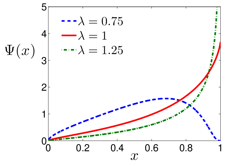
Since the root degree is non self-averaging with $\langle k\rangle\sim N$, we anticipate that when $k,N\to\infty$, the probability distribution $R(k,N)$ admits the scaling form (Fig. 9)

When $\lambda\leq 1$, the scaled distribution $\Psi(x)$ is a smooth function on $[0,1]$, but when $\lambda>1$, $\Psi(x)$ additionally contains a singular component $\mathcal{R}(\lambda)\delta(x-1)$ that accounts for the probability to create a star or a hairball about the root node. Therefore

Consider the extreme behaviors at $x\to 1$. This limit essentially corresponds to the probability of forming the star. Thus for $\lambda=1$ we expect $\Psi(1)=\pi^{-1}\sinh\pi\approx 3.676$. This agrees with simulation results. Further, $\Psi(1)=0$ for $\lambda<1$; more precisely, the scaling function $\Psi(x)$ near $x=1$ is essentially the same as the scaling function $\mathcal{M}_{1}(x)$ describing the largest macrohub, Eq. (17). Hence $\ln\Psi(x)\sim-(1-x)^{-(1-\lambda)}$ as $x\to 1$. This is also compatible with our numerical results.

To estimate the asymptotic behavior of $\Psi(x)$ for $x\to 0$, we have computed the probabilities that the root has the smallest possible degrees $k=3$ and $k=4$ (B). From these results we infer the asymptotic behavior

which is compatible with our numerical results.

The two links created by each new node arise from two qualitatively different mechanisms. One link arises by random attachment, a mechanism that leads to the random recursive tree. The second link is to one of the two parents, and it is selected via enhanced redirection which, as we have shown earlier, leads to a broad and non-extensive degree distribution, $N_{k}\sim N^{\nu-1}/k^{\nu}$ with $\nu<2$. Because of the competition between these two mechanisms, one may anticipate that $N_{k}$ scales linearly with $N$ for sufficiently small $k$, while for large $k$ the degree distribution $N_{k}$ scales as $N^{\nu-1}$ with $\nu<2$. This is indeed the case, as illustrated in Fig. 11.

To understand how two different scaling regimes emerge, we study the master equation that governs $N_{k}$ (compare with Eq. (4)):

The terms in the first set of brackets account for attachment to a randomly-selected target. Similarly, the terms in the second set of brackets account for redirection. Here

is the probability that an incoming node attaches to the degree-$k$ parent of a random target, where ${N}(a,b)$ is the number of nodes with parents of degree $a$ and $b$. Thus $\tau_{k}$ is the probability of redirection to a degree-$k$ parent averaged over all $(k-2)N_{k}$ children of this parent node. In (43), the expression $\tau_{k}(k-2)N_{k}/N$ gives the probability that the incoming node initially targets one of the $(k-2)N_{k}$ children of a node of degree $k$ and then redirects to this parent. The term $\delta_{k,2}$ accounts for each newly-created node has degree $2$.

To determine $N_{k}$, we separately analyze Eq. (43) for small and for large $k$. When $k$ is small, we make the ansatz $N_{k}=c_{k}N$ and substitute into Eq. (43). Rearranging, we find the recursion relation for $c_{k}$ for $k>2$:

while $c_{2}=\frac{1}{2}$. This recursion has the product solution

Since redirection to a low degree parent is unlikely, we approximate the redirection probability as $\tau_{k}=0$ for small $k$. With this approximation, the product in Eq. (46) equals to $1$, and the degree distribution reduces to $N_{k}\approx N/2^{(k-1)}$.

For large $k$, we substitute the non-extensive scaling ansatz $N_{k}=c_{k}N^{\nu-1}$ into Eq. (43), and rearrange to obtain the recursion

This gives the product solution

where $\ell$ is the degree above which the non-extensive scaling ansatz is valid. In the limit of large $k$, we approximate $\tau_{k}=1$ in Eq. (48)because the probability of redirection to a high-degree parent node approaches 1. This gives the asymptotic behavior

Combined with the non-extensive ansatz, the degree distribution for large $k$ is $N_{k}\sim N^{\nu-1}/k^{\nu}$. In the above derivation, the precise value of $\ell$ only affects $c_{k}$ up to a multiplicative factor but not the scaling behavior at large $k$.

We now define the crossover degree $k^{*}$ as the value that separates the small-$k$ extensive scaling regime from the large-$k$ non-extensive regime. To estimate $k^{*}$, we find the value at which $N_{k}$ in the small- and large-$k$ approximations coincide. This leads to the transcendental equation $N/2^{(k^{*}-1)}=N^{\nu-1}/(k^{*})^{\nu}$, whose solution gives $k^{*}\sim\ln N$ to lowest order in $N$.

To summarize, the limiting degree distributions are

with $c$ a constant. As shown in Fig. 12, the agreement between this prediction and the degree distribution from Monte Carlo simulations is excellent. The double attachment rule also produces many macrohubs whose degrees grow linearly with $N$ and also obey the same scaling behavior (12) as in single-attachment enhanced redirection.

The new feature of double attachment is that the resulting network contains closed loops. A basic question about this type of network is whether it is homogeneous or highly clustered. We measure the level of clustering by the local clustering coefficient $C_{i}(k)$ [7] for a given node $i$ of degree $k$. This quantity is defined as the ratio of the actual number of links between the neighbors of node $i$ to the $k(k-1)/2$ possible links between these neighbors if they were all connected. For the complete graph, the local clustering coefficient equals 1 for every node, while in a tree network the local clustering coefficient is everywhere zero.

To compute the local clustering coefficient for double attachment networks, consider an arbitrary node $i$ with degree $k$. There are two ways that attachment can occur to this node: (i) a new node can attach directly to node $i$ and to one of its parents, or (ii) a new node can attach to one of the $k-2$ children of node $i$ and to node $i$ itself. In either case, the degree of node $i$ increases by one and the number of links between the neighbors of node $i$ also increase by one. When node $i$ is first created it necessarily has degree 2 and a single link between its neighbors. Thus when node $i$ reaches degree $k$, it will have $k-1$ links between its neighbors. Therefore its clustering coefficient is $C_{i}(k)=(k-1)/[k(k-1)/2]=2/k$. This $1/k$ scaling of the local clustering coefficient is seen in many real-world networks [39, 40, 41, 42].

The average local clustering coefficient is therefore

This large value for this coefficient value indicates a highly clustered network. For comparison, empirical studies found $\langle C_{i}\rangle=0.79$ for actor collaboration networks [39], $0.68$ for co-authorship networks [40], and $0.14$ for blogging networks [41]. By contrast, the Erdős-Rényi random graphs have a vanishing mean local clustering coefficient; more precisely it decreases with $N$ according to $\langle C_{i}\rangle\sim N^{-1}$ [42].

References

- [1] G. U. Yule, Phil. Trans. Roy. Soc. B 213, 21 (1925).
- [2] H. A. Simon, Biometrika 42, 425 (1955).
- [3] A.-L. Barabási and R. Albert, Science 286, 509 (1999).
- [4] P. L. Krapivsky, S. Redner, and F. Leyvraz, Phys. Rev. Lett. 85, 4629 (2000).
- [5] S. N. Dorogovtsev, J. F. F. Mendes, and A. N. Samukhin, Phys. Rev. Lett. 85, 4633 (2000).
- [6] S. N. Dorogovtsev and J. F. F. Mendes, Evolution of Networks: From Biological Nets to the Internet and WWW (Oxford University Press, Oxford, UK, 2003).
- [7] M. E. J. Newman, Networks: An Introduction (Oxford University Press, Oxford, 2010).
- [8] A. Fabrikant, E. Koutsoupias, and C. H. Papadimitriou, Automata, Languages and Programming, Lecture Notes in Computer Science, 2380, 110, Springer, Berlin, 2002).
- [9] V. Colizza, J. R. Banavar, A. Maritan, and A. Rinaldo, Phys. Rev. Lett. 92, 198701 (2004).
- [10] M. Barthelemy, Phys. Rept. 499, 1 (2011).
- [11] F. Papadopoulos, M. Kitsak, M. Ángeles Serrano, M. Boguñá, and D. Krioukov, Nature 489, 537 (2012).
- [12] J. Kleinberg, R. Kumar, P. Raghavan, S. Rajagopalan, and A. Tomkins, in: Proceedings of the International Conference on Combinatorics and Computing, Lecture Notes in Computer Science, Vol. 1627, pp. 1-18 (Springer-Verlag, Berlin, 1999).
- [13] P. L. Krapivsky and S. Redner, Phys. Rev. E 63, 066123 (2001).
- [14] A. Vázquez, Phys. Rev. E 67, 056104 (2003).
- [15] H. Rozenfeld and D. ben-Avraham, Phys. Rev. E 70, 056107 (2004).
- [16] P. L. Krapivsky and S. Redner, Phys. Rev. E 71, 036118 (2005).
- [17] R. Lambiotte and M. Ausloos Europhys. Lett. 77, 58002 (2007).
- [18] E. Ben-Naim and P. L. Krapivsky, J. Stat. Mech. P06004 (2010).
- [19] A. Gabel and S. Redner, J. Stat. Mech. P02043 (2013).
- [20] P. L. Krapivsky and D. Krioukov, Phys. Rev. E 78, 026114 (2008).
- [21] R. F. i Cancho and R. V. Solé, Statistical Mechanics of Complex Networks, no. 625 in Lecture Notes in Physics, p. 114, Springer, Berlin (2003).
- [22] G. Bianconi and A.-L. Barábasi, Phys. Rev. Lett. 86, 5632 (2001); G. Bianconi and A.-L. Barábasi, Europhys. Lett. 54, 436 (2001).
- [23] P. L. Krapivsky and S. Redner, Comput. Netw. 39, 261 (2002).
- [24] D. L. Bryan and M. E. O’Kelly, J. Regional Science, 39, 275 (1999).
- [25] J. J. Han, N. Bertain, T. Hao, D. S. Goldberg, G. F. Berriz, L. V. Zhang, D. Dupay, A. J. M. Walhout, M. E. Cusick, F. P. Roth, and M. Vidal, Nature 430, 88 (2004).
- [26] R. Guimera, S. Mossa, A. Turtschi, and L. A. N. Amaral, Proc. Natl. Acad. Sci. USA 102, 7794 (2005).
- [27] J. Kunegis, M. Blattner, and C. Moser, arXiv:1303.6271.
- [28] P. L. Krapivsky and S. Redner, J. Phys. A 35, 9517 (2002).
- [29] A. Gabel, P. L. Krapivsky, and S. Redner, Phys. Rev. E 88, 050802 (2013).
- [30] P. L. Krapivsky and S. Redner, Phys. Rev. Lett. 89, 258703 (2002).
- [31] E. J. Gumbel, Statistics of Extremes (Columbia University Press, New York, 1958).
- [32] F. Eggenberger and G. Pólya, Z. Angew. Math. Mech. 3, 279 (1923).
- [33] N. Johnson and S. Kotz, Urn Models and Their Applications: An Approach to Modern Discrete Probability Theory, (Wiley, New York, 1977); H. M. Mahmoud, Pólya Urn Models (Chapman & Hall, London, 2008).
- [34] B. Derrida and H. Flyvbjerg, J. Phys. A 20, 5273 (1987); J. Physique 48, 971 (1987); B. Derrida and D. Bessis, J. Phys. A 21, L509 (1988).
- [35] P. G. Higgs, Phys. Rev. E 51, 95 (1995).
- [36] L. Frachebourg, I. Ispolatov, and P. L. Krapivsky, Phys. Rev. E 52, R5727 (1995).
- [37] B. Derrida and B. Jung-Muller, J. Stat. Phys. 94, 277 (1999).
- [38] P. L. Krapivsky, I. Grosse, and E. Ben-Naim, Phys. Rev. E 61, R993 (2000); P. L. Krapivsky, E. Ben-Naim, and I. Grosse, J. Phys. A 37, 2863 (2004).
- [39] D. Watts and S. H. Strogatz, Nature 393, 440 (1998).
- [40] F. J. Acedo, C. Barroso, C. Casanueva, and J. L. Galán, J. Management Studies 43, 970 (2006).
- [41] F. Fu, L. Liu, and L. Wang, Physica A 387, 675 (2008).
- [42] E. Ravasz and A.-L. Barabási, Phys. Rev. E 67, 026112 (2003).
- [43] M. Abramowitz and A. Stegun, Handbook of Mathematical Functions (Dover, New York, 1965).