Effective lattice Polyakov loop theory vs. full $SU(3)$ Yang-Mills at finite temperature

The spectrum of a theory is encoded in its correlation functions. A natural testing ground for the effective action are thus Polyakov loop correlators. Their exponential decay represents the (unrenormalised) free energy of a static quark anti-quark pair [14],

$$\langle L(R)L^{\dagger}(0)\rangle=e^{-F(R,T)/T}\;.$$

(3)

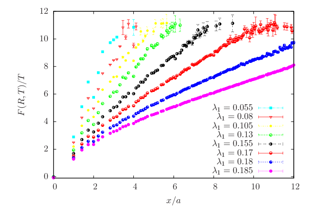
A direct comparison of on-axis correlators between the one-coupling effective theory and full Yang-Mills is shown in figure 1 for two different values of the lattice coupling $\beta$. Note that in the full Yang-Mills simulation an algorithm for exponential error reduction [15] was employed, whereas the data for the effective theory have been obtained only with the comparably small improvement of a multi-hit algorithm. Quantitative agreement is observed for short lattice distances $R/a=0-2$ for $\beta=5.0$, while the effective theory data still follow the general shape of the full correlator, but start to quantitatively deviate for $R/a\geq 2$ at the larger coupling $\beta=5.4$.

Note that the correlators are systematically smaller, i.e. the corresponding free energies are larger in the effective theory. This is shown in continuum units in figure 2, with deviations increasing with distance. The off-axis correlators are also included in this figure. These are a measure for the breaking of rotational invariance by the lattice discretisation, which appears to be amplified in the effective theory compared to the full Yang-Mills theory. This effect gets alleviated when also the next-to-nearest neighbour coupling is included in the effective theory. However, the improvement is small because of the smallness of the effective coupling, with values of $\lambda_{2}(\beta=5.0)=1.9\times 10^{-5}$ and $\lambda_{2}(\beta=5.4)=5.6\times 10^{-5}$, when using its strong coupling expansion eq. (23). On the other hand, when the effective coupling $\lambda_{1}$ (or equivalently $\beta$) is raised, rotational invariance gets restored also in the one-coupling theory, as figure 3 (left) illustrates, i.e. the effective action eventually reproduces the continuum symmetries. In this regime of larger $\lambda_{1}$ just below its critical value, which corresponds to larger $\beta$ and hence finer lattices, it is also possible to distinguish between a linear part at large distances and a Coulomb part at short distances.

Because of the smallness of the effective couplings, it is natural to consider perturbation theory for the effective action. Indeed, the correlator of Polyakov loops can be expressed as a power series in the coupling truncated at $M_{\lambda_{1}}$,

$$\langle L(R)L^{\dagger}(0)\rangle\approx\sum_{n=1}^{M_{\lambda_{1}}}N_{n}(R/a)\lambda_{1}^{l_{n}(R/a)}\;.$$

(4)

If the distance $R/a$ is greater than zero, $l_{1}$ is the “taxi-driver” distance on the lattice, i.e. the minimal number of links connecting the two correlated points. The coefficient functions $N_{n}$ count the number of possible paths of length $l_{n}$ that connect the correlated points. They have been estimated with a numerical algorithm and are summarized in Table 2.

Figure 3 (left) illustrates how for small values of $\lambda_{1}$, i. e. at strong coupling, this analytic result fully reproduces the numerical simulations of the effective model. With growing values of $\lambda_{1}$ and larger distances, higher orders in the expansion become important. At the largest $\lambda_{1}$ value shown in figure 3, which corresponds at $N_{\tau}=4$ to $\beta\approx 6$, the fourth order expansion is still a good approximation for the short distance correlation.

The linear part of the free energy corresponds to a temperature dependent effective string tension, which arises from the Boltzmann average over the linear pieces of the excitations of the static potential. This string tension decreases with $\lambda_{1}$ (or $\beta$), which is tantamount to increasing temperature at fixed $N_{\tau}$, in accord with full Yang-Mills theory [16, 17]. To make the comparison quantitative, we fit our correlator in continuum units with the same ansatz used in [16] (details of the functional form are inspired by string models valid at large distances),

	$\displaystyle\frac{F(R,T)}{T}$	$\displaystyle=$	$\displaystyle v_{0}+\frac{1}{2}\ln(1+(2RT)^{2})+\left[\frac{\pi}{12}-\frac{1}{6}\arctan(2RT)\right]\frac{1}{RT}$		(5)
			$\displaystyle+\left[\frac{\sigma(T)}{T^{2}}-\frac{\pi}{3}+\frac{2}{3}\arctan\left(\frac{1}{2RT}\right)\right]RT\;.$

At short distances $R<T^{-1}$ the temperature effects disappear and the free energy is dominated by its ground state, the static potential of the vacuum,

$$F(R,T)\stackrel{{\scriptstyle R\rightarrow 0}}{{\longrightarrow}}V(R)=c_{1}+\frac{c_{2}}{R}+\sigma R\;.$$

(6)

Data from the effective theory close to the phase transition, $T=0.90T_{c}$ are shown in figure 4 (left). They are well described by the finite temperature fit in the long distance region while being also compatible with the corresponding vacuum fit function appropriate for short distances. Thus, the qualitative features of the free energy of Yang-Mills theory are reproduced. However, the numerical values for the temperature dependent string tension for $N_{\tau}=6$ are significantly overestimated. A collection of fit results in comparison with the full answer is shown in figure 4 (right). We see that on $N_{\tau}=4$ the results are closer to the true answer and that the effective theory prediction seems to grow with $N_{\tau}$.

This incorrect scaling behaviour of the effective string tension is an artefact of the one-coupling theory. For all parirings $(\beta,N_{\tau})$ with constant effective coupling $\lambda_{1}(\beta,N_{\tau})$ the correlators as a function of distance in lattice units are the same. At large $R$ this implies that for two different $N_{\tau}$ with the same value of $\lambda_{1}$ the string tensions are related by

$$\left(\frac{\sigma(T_{1})}{T_{1}^{2}}+\frac{\pi}{3}\right)\frac{1}{(N_{\tau})_{1}}=\left(\frac{\sigma(T_{2})}{T_{2}^{2}}+\frac{\pi}{3}\right)\frac{1}{(N_{\tau})_{2}}\;,$$

(7)

where the temperatures are determined by the corresponding $N_{\tau}$ and $\beta$. (The scale is set such that $T((\lambda_{1})_{c})=T_{c}$ for all $N_{\tau}$). This forces the string tension to scale approximately with $N_{\tau}$ in the region close to $T_{c}$. The solution is an effective theory with more than one coupling constant. Then there is a critical (hyper-)surface and at each $N_{\tau}$ the phase transition can occur at a different values of the coupling constants. Our strong coupling result for the next-to-nearest neighbour interaction alone is however too small for a significant change of the string tension close to the phase transition.

One can understand qualitatively, why the value of the string tension cannot be correctly predicted by an effective theory with only a few couplings. We have already seen that the correlators are increasingly underestimated as the correlation distance in lattice units grows. A fixed distance in physical units contains more and more lattice spacings as the lattice gets finer. Correspondingly, the effective theory with a fixed number of couplings covers an ever smaller contribution to the correlator at fixed distance correctly. While the higher order couplings do become parametrically smaller $\sim u^{nN_{\tau}+m}$, eq. (22), a rapidly increasing number of them contributes to a correlator at distance $R/a$. Moreover, their apparent suppression with $N_{\tau}$ cancels in the contribution to the free energy. This can be demonstrated rather precisely by considering the strong coupling expansion of the vacuum string tension, i.e. the limit $N_{\tau}\rightarrow\infty$ at fixed $\beta$. The expansion starting from the 4d Yang-Mills theory is well known [18] (for a finite temperature version, see [19]),

$$a^{2}\sigma|_{\textrm{YM}}=-\ln u-4u^{4}-12u^{5}+10u^{6}+O(u^{7})$$

(8)

On the other hand, expanding the 3d effective theory in powers of the effective coupling constant $\lambda_{1}$ we obtain from the on-axis correlator

$$a^{2}\sigma|_{\textrm{eff.th.}}=-\frac{1}{N_{\tau}}\ln(\lambda_{1})-\frac{2\lambda_{1}}{N_{\tau}}+\ldots=-\ln u-4u^{4}-12u^{5}+14u^{6}+O(u^{8})\;.$$

(9)

Only the first two terms agree with the expansion of the full theory. Note how the $N_{\tau}$-dependence of $\lambda_{1}$ is cancelled by an explicit $N_{\tau}$-dependence, while the second term is, as $\lambda_{1}$ itself, exponentially suppressed for increasing $N_{\tau}$. If we also include $\lambda_{3}$, the coupling for on-axis neighbours at distance $R/a=2$, we obtain instead

	$\displaystyle a^{2}\sigma|_{\textrm{eff.th.}}$	$\displaystyle=$	$\displaystyle-\frac{1}{N_{\tau}}\ln(\lambda_{1})-\frac{2\lambda_{1}^{2}}{N_{\tau}}-\frac{\lambda_{3}\lambda_{1}^{-2}}{N_{\tau}}+\sum_{n=2}^{\frac{1}{2}(R/a-1)}c_{n}\lambda_{3}^{n}\lambda_{1}^{-2n}\ldots$		(10)
		$\displaystyle=$	$\displaystyle-\ln u-4u^{4}-12u^{5}+10u^{6}+O(u^{8})\;.$

The detailed form of the last term in the first line depends on whether $R/a$ is even or odd, but the number of terms in the sum scales with $R/a$. Because of the $N_{\tau}$-dependence of the couplings, the second term is less significant than the third one for larger $N_{\tau}$. The leading contribution of the third term is $4u^{6}$, such that the string tension is now correctly reproduced through order $u^{6}$. Correspondingly, the coefficients of higher orders receive more and more contributions from long-range couplings.

We conclude that the long-range interactions may not be neglected in the computation of correlation functions within the effective theory. Contrary to the effective couplings themselves, their contribution to correlators are not suppressed by $N_{\tau}$ and without them the coefficients of the strong coupling expansion of correlators are incomplete. While we have used the strong coupling expansion to show this, we stress that the conclusion is independent of the way the effective theory is determined or used, and in complete agreement with the non-perturbative observations made in [7].

In this section we test the description of bulk thermodynamic quantities by the effective theory, which are all derived from the partition function directly. The fundamental ingredient to the equation of state is the free energy density in units of the temperature. In homogeneous systems it is related to the pressure $p$ as

$$\frac{f}{T^{4}}=\frac{-p}{T^{4}}=-\frac{\ln Z}{VT^{3}}\;.$$

(11)

For the correct renormalisation the divergent zero temperature part has to be subtracted.

In order to judge the quality of the effective theory, it is again instructive to consider the strong coupling expansion for different versions of the action,

	4d YM:		$\displaystyle\phantom{f(\lambda_{1}(u,N_{\tau}))}f(u,N_{\tau})=-\frac{6}{N_{\tau}}u^{4N_{\tau}}+\ldots\;,$		(12)
	eff. theory, linear action:		$\displaystyle\phantom{f(u,N_{\tau})}f(\lambda_{1}(u,N_{\tau}))=-\frac{3}{N_{\tau}}\lambda_{1}^{2}+\ldots=-\frac{3}{N_{\tau}}u^{2N_{\tau}}+\ldots\;,$
	eff.theory, log. action:		$\displaystyle\phantom{f(u,N_{\tau})}f(\lambda_{1}(u,N_{\tau}))=-\frac{6}{N_{\tau}}\lambda_{1}^{4}+\ldots=-\frac{6}{N_{\tau}}u^{4N_{\tau}}+\ldots\;.$

Here the full action is the ordinary strong coupling expansion without the detour of the effective theory [20, 21], the log. action corresponds to the first term of eq. (2) and the linear action to its leading term in $\lambda_{1}$ only. The explicit comparison reveals that the resummation of higher power terms into the logarithm is necessary to correctly reproduce the leading term of the full theory.

In a lattice simulation all expectation values are normalised on the partition function, which thus cannot be calculated directly. The free energy density is computed indirectly through its derivative with respect to the coupling constant $\beta$, which then has to be integrated over [22, 23, 24],

$$\left.\frac{f}{T^{4}}\right|_{\beta_{0}}^{\beta}=-\int_{\beta_{0}}^{\beta}d\beta^{\prime}\Delta S(\beta^{\prime})\;,$$

(13)

with the interaction measure

$$\Delta S(\beta)=\frac{1}{T^{4}}\left(\left.\frac{T}{V}\frac{d\ln Z}{d\beta}\right|_{T}-\left.\frac{T}{V}\frac{d\ln Z}{d\beta}\right|_{T=0}\right)=\frac{6N_{\tau}^{4}}{N_{c}}\left(\langle\mathrm{Re}P\rangle|_{T}-\langle\mathrm{Re}P\rangle|_{T=0}\right)\;.$$

(14)

Thus, all information of the equation of state is encoded in $\Delta S$. Computationally, this is a simple subtraction of two plaquette ($P$) expectation values averaged over all orientations and volume. Finite temperature $T$ and $T=0$ are represented in terms of a $N_{\tau}\times N_{s}^{3}$ and a $N_{s}^{4}$ lattice with $N_{s}=4N_{\tau}$.

The strong coupling expansion for $\Delta S$ can be obtained from the series for the pressure [3],

$$\Delta S=N_{\tau}^{4}\frac{d(a^{4}p)}{d\beta}=N_{\tau}^{4}K(u,N_{\tau})\frac{du}{d\beta}\;,$$

(15)

where for $N_{\tau}=2,4$ we have

	$\displaystyle K(u,N_{\tau}=4)$	$\displaystyle=24u^{15}+1458u^{17}-5643u^{18}+9945u^{19}-\frac{201285}{4}u^{20}$
		$\displaystyle+\frac{360638553}{1024}u^{21}-\frac{8627830587}{10240}u^{22}+\frac{6648458901}{5120}u^{23}\;,$
	$\displaystyle K(u,N_{\tau}=2)$	$\displaystyle=24u^{7}+270u^{9}-1485u^{10}+3315u^{11}-\frac{4563}{4}u^{12}+\frac{126411873}{5120}u^{13}$
		$\displaystyle-\frac{221629365}{2048}u^{14}+\frac{648558969807}{5242880}u^{15}\;.$		(16)

This can be compared with the data of the effective Polyakov loop action and the full theory. In the effective theory we compute

	$\displaystyle\Delta S(\beta)$	$\displaystyle=$	$\displaystyle\frac{1}{T^{4}}\sum_{n}\left(\left.\frac{T}{V}\frac{d\ln Z}{d\lambda_{n}}\frac{d\lambda_{n}}{du}\right|_{\{\lambda_{n}=\lambda_{n}[N_{\tau},u]\}}-\left.\frac{T}{V}\frac{d\ln Z}{d\lambda_{n}}\frac{d\lambda_{n}}{du}\right|_{\{\lambda_{n}=\lambda_{n}[N_{s},u]\}}\right)\frac{du}{d\beta}$		(17)
		$\displaystyle=$	$\displaystyle 3N_{\tau}^{4}\left(\frac{1}{N_{\tau}}\left.\langle R_{1}(\{\lambda_{i}\})\rangle\frac{d\lambda_{1}}{du}\right|_{\lambda_{1}=\lambda_{1}[N_{\tau},u]}-\frac{1}{N_{s}}\left.\langle R_{1}(\{\lambda_{i}\})\rangle\frac{d\lambda_{1}}{du}\right|_{\lambda_{1}=\lambda_{1}[N_{s},u]}\right)\frac{du}{d\beta}$
			$\displaystyle+3N_{\tau}^{4}\sum_{n=2}\left(\frac{1}{N_{\tau}}\left.\langle R_{n}(\{\lambda_{i}\})\rangle\frac{d\lambda_{n}}{du}\right|_{\lambda_{i}=\lambda_{i}[N_{\tau},u]}-\frac{1}{N_{s}}\left.\langle R_{n}(\{\lambda_{i}\})\rangle\frac{d\lambda_{n}}{du}\right|_{\lambda_{i}=\lambda_{i}[N_{s},u]}\right)\frac{du}{d\beta}\;.$

where all expectation values are calculated on a $N_{s}^{3}$ lattice and $\langle R_{n}\rangle=1/(3N_{s}^{3})d\ln Z/d\lambda_{n}$. In the one-coupling theory the last equation reduces to the first line with

$$R(\lambda_{1})=\frac{1}{3N_{s}^{3}}\sum_{<i,j>}\frac{2\mathrm{Re}(L_{i}L^{\dagger}_{j})}{1+2\lambda_{1}\mathrm{Re}(L_{i}L^{\dagger}_{j})}\;.$$

(18)

Again an expansion in the limit of small $\lambda_{1}$ provides a good check of the results. The expectation value of $R$ has a simple form in this limit, where it is dominated by the nearest-neighbour contribution between adjacent points ($i,j$) on the lattice,

$$\langle R_{1}(\lambda_{1})\rangle\approx 2\Big(4\lambda_{1}^{3}+44\lambda_{1}^{5}+O(\lambda_{1}^{6})\Big)\;.$$

(19)

In this approximation finite volume corrections have been neglected.

We can now appreciate the difference to the situation for the string tension. Comparing eqs. (17), (15), we see that they both have the same trivial $N_{\tau}^{4}$-dependence as a prefactor. Any other dependence on $N_{\tau}$ in eq. (17) is contained in the $\lambda_{n}$. Once again mixed polynomials in the $\lambda_{n}$ are needed to reproduce higher coefficients of the 4d strong coupling expansion, but the power counting in $u$ can be based on that of the $\lambda_{n}$ directly, without cancellations of $N_{\tau}$-dependences as in the case of the string tension. The reason is that in the derivation of the effective theory the "observable" computed as a strong coupling series is the effective action itself, and thus the partition function. These analytic considerations are borne out by numerical simulations.

Unfortunately, the numerical determination of this quantity is quite difficult due to large cancellations in the subtraction, which implies a small signal-to-noise ratio. Particularly in the region of strong coupling (small $\beta$), $\Delta S$ drops exponentially causing a corresponding growth of the signal to noise ratio. For an overview and references, see [25]. It is then hard to bridge the gap between analytic strong coupling predictions [3] and simulations. In this regime the effective theory turns out to be very useful. Numerical results for $\Delta S$ as a function of the gauge coupling are shown in figure 5 for $8^{3}\times 2$ and $16^{3}\times 4$ lattices. The data demonstrate the advantage of the effective theory. Due to the larger statistics obtained in simple three dimensional simulations a much higher precision can be achieved than in the full theory. This allows to extend the considered $\beta$-range towards smaller values, in particular for higher $N_{\tau}$ where this is impossible in the full theory. This corresponds to the region of lower temperatures. We observe excellent quantitative agreement over a wide $\beta$-range. Deviations between full and effective theory predictions only set in at the deconfinement phase transition, with $\beta^{c}<\beta_{c}^{\mathrm{eff}}$, cf. table 1.

In figure 5 we also compare with the fully analytic results of the strong coupling expansion and the expansion in small $\lambda_{1}$ within the effective theory. In a large $\beta$-range the small $\lambda_{1}$ expansion gives an excellent description. This indicates that for bulk quantities the short range interactions are dominant in the region well below the phase transition. Note that the $\lambda_{1}$-expansion is a much better approximation than the strong coupling series for the pressure in [21]. These two results converge, of course, in the strong coupling limit. At larger $\beta$ the use of the effective theory entails non-perturbative resummations compared to the straightforward strong coupling expansion, leading to an improved convergence towards the full theory.

While the critical couplings for the deconfinement transtion, table 1, have already been determined in [3], we would like to discuss here why the effective theory works so well for this observable. In statistical mechanics, a standard observable to locate a phase boundary is the generalised susceptibility of an observable $O({\mathbf{x}})$,

$$\chi_{O}=\int d^{3}x\left(\langle O({\mathbf{x}})O(0)\rangle-\langle O({\mathbf{x}})\rangle\langle O(0)\rangle\right).$$

(20)

At a phase transition fluctuations are maximal, hence the peaks of susceptibilities define (pseudo-) critical couplings, whose finite size scaling moreover contains information about the order and universality class of the transition. The important observation is that, despite the integration over all distances, eq. (20) is a local observable for any theory with a mass gap. The correlators decay exponentially with distance,

$$\langle O({\mathbf{x}})O(0)\rangle\sim\sum_{n}c_{n}^{2}e^{-E_{n}|{\mathbf{x}}|}\;,$$

(21)

with some energy eigenvalues $E_{n}$ and matrix elements $c_{n}$, such that the integral is dominated by the contact and short distance contributions. Moreover, at phase transitions the correlation length of a system either diverges (second order) or is maximal (first order and crossover), which implies that any scales smaller than the correlation length play either no or only a suppressed role. On the other hand, the behaviour of the correlation length is dictated by the symmetries and dimensionality of the theory. A similar reasoning applies for bulk thermodynamic quantities, which are derived from the partition function. The non-trivial quantity to compute in this case is the action, which again is local in the sense that couplings over larger distances are exponentially suppressed. Thus, a local effective action with the correct symmetries is capable to provide a good description of bulk thermodynamic quantities as well as phase transitions, even though it might be inaccurate for specific correlation functions or the spectrum of the theory.

References

- (1) T. K. Herbst, M. Mitter, J. M. Pawlowski, B. -J. Schaefer and R. Stiele, arXiv:1308.3621 [hep-ph].
- (2) A. Vuorinen and L. G. Yaffe, Phys. Rev. D 74 (2006) 025011 [hep-ph/0604100].
- (3) J. Langelage, S. Lottini and O. Philipsen, JHEP 1102 (2011) 057 [Erratum-ibid. 1107 (2011) 014] [arXiv:1010.0951 [hep-lat]].
- (4) A. S. Christensen, J. C. Myers and P. D. Pedersen, arXiv:1312.3519 [hep-lat].
- (5) C. Wozar, T. Kaestner, A. Wipf and T. Heinzl, Phys. Rev. D 76 (2007) 085004 [arXiv:0704.2570 [hep-lat]].
- (6) J. Greensite and K. Langfeld, Phys. Rev. D 88 (2013) 074503 [arXiv:1305.0048 [hep-lat]].
- (7) J. Greensite and K. Langfeld, Phys. Rev. D 87 (2013) 094501 [arXiv:1301.4977 [hep-lat]].
- (8) C. S. Fischer, L. Fister, J. Luecker and J. M. Pawlowski, arXiv:1306.6022 [hep-ph].
- (9) J. Fingberg, U. M. Heller and F. Karsch, Nucl. Phys. B 392 (1993) 493.
- (10) J. Kogut, M. Stone and H. W. Wyld, Phys. Rev. Lett. 50 (1983) 393.
- (11) A. Francis, O. Kaczmarek, M. Laine, M. Müller, T. Neuhaus and H. Ohno, arXiv:1311.3759 [hep-lat].
- (12) S. Necco and R. Sommer, Nucl. Phys. B 622 (2002) 328 [hep-lat/0108008].
- (13) M. Fromm, J. Langelage, S. Lottini and O. Philipsen, JHEP 1201 (2012) 042 [arXiv:1111.4953 [hep-lat]].
- (14) L. D. McLerran and B. Svetitsky, Phys. Rev. D 24 (1981) 450.
- (15) M. Lüscher and P. Weisz, JHEP 0109 (2001) 010 [hep-lat/0108014].
- (16) O. Kaczmarek, F. Karsch, E. Laermann and M. Lutgemeier, Phys. Rev. D 62 (2000) 034021 [hep-lat/9908010].
- (17) N. Cardoso and P. Bicudo, Phys. Rev. D 85 (2012) 077501 [arXiv:1111.1317 [hep-lat]].
- (18) I. Montvay and G. Münster, Cambridge, UK: Univ. Pr. (1994) 491 p. (Cambridge monographs on mathematical physics)
- (19) F. Green, Nucl. Phys. B 215 (1983) 83.
- (20) J. Langelage, G. Münster and O. Philipsen, JHEP 0807 (2008) 036 [arXiv:0805.1163 [hep-lat]].
- (21) J. Langelage and O. Philipsen, JHEP 1004 (2010) 055 [arXiv:1002.1507 [hep-lat]].
- (22) J. Engels, F. Karsch, H. Satz and I. Montvay, Nucl. Phys. B 205 (1982) 545.
- (23) J. Engels, J. Fingberg, F. Karsch, D. Miller and M. Weber, Phys. Lett. B 252 (1990) 625.
- (24) G. Boyd, J. Engels, F. Karsch, E. Laermann, C. Legeland, M. Lutgemeier and B. Petersson, Nucl. Phys. B 469 (1996) 419 [hep-lat/9602007].
- (25) O. Philipsen, Prog. Part. Nucl. Phys. 70 (2013) 55 [arXiv:1207.5999 [hep-lat]].
- (26) M. Fromm, J. Langelage, S. Lottini, M. Neuman and O. Philipsen, Phys. Rev. Lett. 110 (2013) 12, 122001 [arXiv:1207.3005 [hep-lat]].