Optimal polygonal $L_{1}$ linearization and
fast interpolation of nonlinear systems

Guillermo Gallego Daniel Berjón and Narciso García ^†^†thanks: This work has been partially supported by the Ministerio de Economía y Competitividad of the Spanish Government under project TEC2010-20412 (Enhanced 3DTV). G. Gallego is supported by the Marie Curie - COFUND Programme of the EU (Seventh Framework Programme). G.˜Gallego, D.˜Berjón and N.˜García are with Grupo de Tratamiento de Imágenes (GTI), ETSI Telecomunicación, Universidad Politécnica de Madrid, Madrid, Spain, e-mail: {ggb,dbd,narciso}@gti.ssr.upm.es. Copyright (c) 2014 IEEE. Personal use of this material is permitted. However, permission to use this material for any other purposes must be obtained from the IEEE. DOI: 10.1109/TCSI.2014.2327313

Abstract

The analysis of complex nonlinear systems is often carried out using simpler piecewise linear representations of them. A principled and practical technique is proposed to linearize and evaluate arbitrary continuous nonlinear functions using polygonal (continuous piecewise linear) models under the L1 norm. A thorough error analysis is developed to guide an optimal design of two kinds of polygonal approximations in the asymptotic case of a large budget of evaluation subintervals N. The method allows the user to obtain the level of linearization (N) for a target approximation error and vice versa. It is suitable for, but not limited to, an efficient implementation in modern Graphics Processing Units (GPUs), allowing real-time performance of computationally demanding applications. The quality and efficiency of the technique has been measured in detail on two nonlinear functions that are widely used in many areas of scientific computing and are expensive to evaluate.

Index Terms:

Piecewise linearization, numerical approximation and analysis, least-first-power, optimization.

I Introduction

The approximation of complex nonlinear systems by simpler piecewise linear representations is a recurrent and attractive task in many applications since the resulting simplified models have lower complexity, fit into well established tools for linear systems and are capable of representing arbitrary nonlinear mappings. Examples include, among others, complexity reduction for finding the inverse of nonlinear functions [1, 2], distortion mitigation techniques such as predistorters for power amplifier linearization [3, 4], the approximation of nonlinear vector fields obtained from state equations [5], the obtainment of approximate solutions in simulations with complex nonlinear systems [6], or the search for canonical piecewise linear representations in one and multiple dimensions [7].

In the last decades, the main efforts in piecewise linearization have been devoted both to find approximations of multidimensional functions from a mathematical standpoint and to define circuit architectures implementing them (see, for example, [8] and references therein). In the one-dimensional setting, a simple and common linearization strategy consists in building a linear interpolant between samples of the nonlinear function over a uniform partition of its domain. Such a polygonal (i.e., continuous piecewise linear) interpolant may be further optimized by choosing a better partition of the domain according to the minimization of some error measure. This is a sensible strategy in problems where there is a constraint on the budget of samples allowed in the partition.

Hence, in spite of the multiple benefits derived from modeling with piecewise linear representations, a proper selection of the interval partitions and/or predefining the number of partitions is paramount for a satisfactory performance. Some researchers [2] use cross-validation based approaches to select such a number of pieces within a partition. In other applications, the budget of pieces may be constrained by an internal design requirement (speed, memory or target error) of the approximation algorithm or by some external condition.

Simplified models may be built using descent methods [9], dynamic programming [10] or heuristics such as genetic [1] and/or clustering [11] algorithms to optimize some target approximation error. In some cases, however, the resulting piecewise representation may fail to preserve desirable properties of the original nonlinear system such as continuity [1].

We consider the simplified model representation given by the least-first-power or best $L_{1}$ approximation of a continuous nonlinear function $f$ by some polygonal function. The generic topic of least-first-power approximation has been previously considered in several references, e.g., [12, 13, 14], over a span of many years and it is a recurrent topic and source of insightful results.

We develop a fast and practical method to compute a suboptimal partition of the interval where the polygonal interpolant and the best $L_{1}$ polygonal approximation to a nonlinear function are to be computed. This technique allows to further optimize the $L_{1}$ polygonal approximation to a function among all possible partitions having the same number of segments, or conversely, allow to achieve a target approximation error while minimizing the budget of segments used to represent the nonlinear function. The resulting polygonal approximation is useful in applications where the evaluation of continuous mathematical functions constitutes a significant computational burden, such as computer vision [15, 16] or signal processing [17, 18, 19].

Our work may be generalized to the linearization of multidimensional functions [7] and the incorporation of constraints, thus opening new perspectives also in the context of designing circuit architectures for such piecewise linear approximations, as in [8]. However, these interesting generalizations will be the topic of future work.

The paper is organized as follows: two polygonal approximations of real-valued univariate functions (interpolant and best $L_{1}$ approximation) are presented in Section II. The mathematical foundation and algorithmic procedure to compute a suboptimal partition for the polygonal approximations are developed in Section III. The implementation of the numerical evaluation of polygonal approximations is discussed in Section IV. Experimental results of the developed technique on nonlinear functions (Gaussian, chirp) are given in Section V, both in terms of quality and computational times. Finally, some conclusions are drawn in Section VI.

II Piecewise Linearization

Refer to caption — Figure 1: Top: seventh degree polynomial $f(x)=(x+4)(x+3)(x+2.5)x(x-1.5)(x-2)(x-3)$ and two polygonal approximations: the linear interpolant $\pi_{T}f$ and the best $L_{1}$ approximation $\hat{f}$ . Bottom: corresponding absolute approximation errors (magnified by a $5\times$ factor).

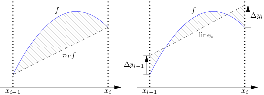
In general, a piecewise function over an interval $I=[a,b]$ is specified by two elements: a set of control or nodal points $\{x_{i}\}_{i=0}^{N}$ , also called knots, that determine a partition $T=\{I_{i}\}_{i=1}^{N}$ of $I$ into a set of $N$ (disjoint) subintervals $I_{i}=[x_{i-1},x_{i}]\mid a=x_{0}<x_{1}<\ldots<x_{N}=b$ , and a collection of $N$ functions $f_{i}(x)$ (so called “pieces”), one for each subinterval $I_{i}$ . In particular, a polygonal or continuous piecewise linear (CPWL) function satisfies additional constraints: all “pieces” $f_{i}(x)$ are (continuous) linear segments and there are no jumps across pieces, i.e., continuity is also enforced at subinterval boundaries, $f_{i}(x_{i})=f_{i+1}(x_{i})\;\forall i=\left\{1,\ldots,N-1\right\}$ . Fig. 1 shows, for a given partition $T,$ the two polygonal functions that we use throughout the paper to approximate a real-valued function $f$ : the interpolant $\pi_{T}f$ and best $L_{1}$ approximation $\hat{f}$ . Polygonal functions of a given partition $T$ generate a vector space $\mathrm{V}_{T}$ since the addition of such functions and/or multiplication by a scalar yields another polygonal function defined over the same partition.

A useful basis for vector space $\mathrm{V}_{T}$ is formed by the set of nodal basis or hat functions $\left\{\varphi_{i}\right\}_{i=0}^{N}$ , where $\varphi_{i}$ , displayed in Fig. 2, is the piecewise linear function in $\mathrm{V}_{T}$ whose value is 1 at $x_{i}$ and zero at all other control points $x_{j}$ , $j\neq i$ , i.e.,

\varphi_{i}(x)=\begin{cases}\frac{x-x_{i-1}}{x_{i}-x_{i-1}}&\text{if }x\in[x_{i-1},x_{i}],\\ \frac{x_{i+1}-x}{x_{i+1}-x_{i}}&\text{if }x\in[x_{i},x_{i+1}],\\ 0&\text{otherwise}.\end{cases}

Functions $\varphi_{0}$ and $\varphi_{N}$ associated to boundary points $x_{0}$ and $x_{N}$ are only half hats. These basis functions are convenient since they can represent any function $v\in\mathrm{V}_{T}$ in terms of the values of $v$ at the control points, $v_{i}=v(x_{i})$ , in the form

v(x)=\sum_{i=0}^{N}v_{i}\varphi_{i}(x).

(1)

From an approximation point of view this basis is frequently used in the Finite Element Method since the hat function (simplex in arbitrary dimensions) is flexible, economic and in some way a natural geometrical element into which to decompose an arbitrary geometric object.

The polygonal interpolant $\pi_{T}f\in\mathrm{V}_{T}$ of a continuous function $f$ (possibly not in $\mathrm{V}_{T}$ ) over the interval $I$ linearly interpolates the samples of $f$ at the control points, thus using $v_{i}=f(x_{i})$ in (1),

\pi_{T}f(x)=\sum_{i=0}^{N}f(x_{i})\varphi_{i}(x).

This polygonal approximation is trivial to construct and might be good enough in some applications (e.g., power amplifier predistorters [4], the trapezoidal rule for integration), but for us it is useful to analyze other possible polygonal approximations, such as the best one in the $L_{1}$ sense, as we discuss next.

Now, consider the problem of approximating a continuous function $f$ by some polygonal function in $\mathrm{V}_{T}$ using the $L_{1}$ norm to measure distances. We address natural questions such as the existence and uniqueness of such a best approximation, methods to determine it and the derivation of estimates for the minimal distance.

Let us answer the question about the existence of a best approximation, i.e., the existence of $\hat{f}\in\mathrm{V}_{T}$ whose distance from $f$ is least. Recall that the space of continuous functions in a given closed interval $I=[a,b]$ , together with the $L_{1}$ norm

\|u\|_{L_{1}(I)}\coloneqq\int_{I}|u(x)|\,\mathrm{d}x

(2)

is a normed linear vector space (NLVS) $(C(I),\|\cdot\|_{L_{1}(I)})$ . Since $\mathrm{V}_{T}\subset C(I)$ is a finite dimensional linear subspace (with basis given by the nodal functions $\{\varphi_{i}\}$ ) of the normed space $(C(I),\|\cdot\|_{L_{1}(I)})$ , then for every $f\in C(I)$ there exists a best approximation to $f$ in $\mathrm{V}_{T}$ [20, Cor. 15.10] [21, Thm. I.1].

The uniqueness of the best approximation is guaranteed for strictly convex subspaces of NLVSs [20, Thm. 15.19] [21, Thm. I.3], i.e., those whose unit balls are strictly convex sets. Linear vector spaces with the 1 or $\infty$ norms are not strictly convex, therefore (a priori) the solution might be unique, but it is not guaranteed. In these cases, the uniqueness question requires special consideration. Further insights about this topic are given in [22, ch. 4][21, ch. 3], which are general references for $L_{1}$ approximation (using polynomials or other functions) and in [23], which is a comprehensive and advanced reference about nonlinear approximation.

Next, we show how to compute such a best $L_{1}$ approximation, and later we will carry out an error analysis. As is well known [24, p. 130], generically, the analytic approach to optimization problems using the $L_{1}$ norm involves derivatives of the absolute value, which makes the search for an analytical solution significantly more difficult than other problems (e.g., those using the $L_{2}$ norm).

As already seen, a function $v\in\mathrm{V}_{T}$ can be written as (1). Let us explicitly note the dependence of $v$ with respect to the coefficients $\mathbf{v}=(v_{0},\ldots,v_{N})^{\top}$ by $v(x)\equiv v(x;\mathbf{v})$ . The least-first-power or best $L_{1}$ approximation to $f\in C(I)$ is a function $\hat{f}\in\mathrm{V}_{T}$ that minimizes $\|f-\hat{f}\|_{L_{1}(I)}$ . Since $\hat{f}\in\mathrm{V}_{T}$ , it admits the expansion in terms of the basis functions of $\mathrm{V}_{T}$ , i.e., letting $\mathbf{y}=(y_{0},\ldots,y_{N})^{\top}$ we may write

\hat{f}(x)\equiv\hat{f}(x;\mathbf{y})=\sum_{i=0}^{N}y_{i}\varphi_{i}(x).

(3)

By definition, the coefficients $\mathbf{y}$ minimize the cost function

\text{cost}(\mathbf{v})\coloneqq\|f(x)-\hat{f}(x;\mathbf{v})\|_{L_{1}(I)}.

(4)

Hence, they solve the necessary optimality conditions given by the non-linear system of $N+1$ equations

\mathbf{g}(\mathbf{v})\coloneqq\frac{\partial}{\partial\mathbf{v}}\text{cost}(\mathbf{v})=\mathbf{0},

(5)

where $\mathbf{g}=(g_{0},\ldots,g_{N})^{\top}$ is the gradient of (4), with entries $g_{j}(\mathbf{v})=\frac{\partial}{\partial v_{j}}\text{cost}(\mathbf{v})$ .

Due to the partition of the interval $I$ into disjoint subintervals $I_{i}=[x_{i-1},x_{i}]$ , we may write (4) as

	$\displaystyle\text{cost}(\mathbf{v})$	$\displaystyle=\sum_{i=1}^{N}\\|f(x)-\hat{f}(x;\mathbf{v})\\|_{L_{1}(I_{i})}$
		$\displaystyle=\sum_{i=1}^{N}\int_{I_{i}}\left\|f(x)-\left(v_{i-1}\varphi_{i-1}(x)+v_{i}\varphi_{i}(x)\right)\right\|\mathrm{d}x,$

therefore, if $\text{sign}(x)=x/|x|$ , each gradient component is,

	$\displaystyle g_{j}(\mathbf{v})=$	$\displaystyle-\int_{I_{j}}\text{sign}\Bigl(f(x)-\sum_{n=j-1}^{j}v_{n}\varphi_{n}(x)\Bigr)\varphi_{j}(x)\,\mathrm{d}x$
		$\displaystyle-\int_{I_{j+1}}\text{sign}\Bigl(f(x)-\sum_{n=j}^{j+1}v_{n}\varphi_{n}(x)\Bigr)\varphi_{j}(x)\,\mathrm{d}x.$

Observe that $g_{j}$ solely depends on $\{v_{j-1},v_{j},v_{j+1}\}$ (except at extreme cases $j=\{0,N\}$ ) due to the locality and adjacency of the basis functions $\{\varphi_{i}\}$ . In the case of the $L_{2}$ norm, the optimality conditions are linear and the previous observation leads to a tridiagonal (linear) system of equations.

A closed form solution of (5) may not be available, and so, to solve the system we use standard numerical iterative algorithms of the form $\mathbf{v}^{k+1}=\mathbf{v}^{k}+\mathbf{s}^{k}$ to find an approximate local solution $\mathbf{y}=\lim_{k\to\infty}\mathbf{v}^{k}$ . Specifically, we use step $\mathbf{s}^{k}$ in the Newton-Raphson iteration given by the solution of the linear system $\mbox{H}(\mathbf{v}^{k})\,\mathbf{s}^{k}=-\mathbf{g}(\mathbf{v}^{k})$ , where $\mbox{H}=\frac{\partial\mathbf{g}}{\partial\mathbf{v}}$ . Near the solution $\mathbf{y}$ , this iteration has quadratic convergence rate. This is also the step given by Newton’s optimization method when approximating (4) by its quadratic Taylor model. Due to the locality of the basis functions $\{\varphi_{i}\}$ , cost function (4) has the advantage that its Hessian (H) is a tridiagonal matrix, so $\mathbf{s}^{k}$ is faster to compute than in the case of a full Hessian matrix.

The search for the optimal coefficients may be initialized by setting $\mathbf{v}^{0}$ equal to the values of the function at the nodal points, i.e., $\mathbf{v}^{0}=(v_{0}^{0},\ldots,v_{N}^{0})^{\top}$ with $v_{i}^{0}=f(x_{i})$ . A more sensible initialization $\mathbf{v}^{0}$ to improve convergence toward the optimal coefficients is given by the ordinates $\mathbf{v}^{0}=\mathbf{c}=(c_{0},\ldots,c_{N})^{\top}$ of the best $L_{2}$ approximation (i.e., orthogonal projection of $f$ onto $\mathrm{V}_{T}$ ) $P_{T}f(x)=\sum_{i=0}^{N}c_{i}\varphi_{i}(x)$ , which are easily obtained by solving a linear system of equations using the Thomas algorithm, $M\mathbf{c}=\mathbf{b}$ with tridiagonal Gramian matrix $M=(m_{ij}),$ $m_{ij}=\left\langle\varphi_{i},\varphi_{j}\right\rangle$ , $\mathbf{b}=(b_{0},\ldots,b_{N})^{\top}$ , $b_{i}=\left\langle f,\varphi_{i}\right\rangle$ and inner product $\left\langle u,v\right\rangle\coloneqq\int_{I}u(x)v(x)\mathrm{d}x$ .

From a numerical point of view, it is also a reasonable choice to replace $\text{sign}(x)$ by some smooth approximation, for example, $\text{sign}(x)\approx\tanh(kx)$ , with parameter $k\gg 1$ controlling the width of the transition around $x=0$ .

In summary, the coefficients $\mathbf{y}$ that specify the best $L_{1}$ approximation (3) on a given partition $T$ are computed numerically via iterative local optimization techniques starting from an initial guess $\mathbf{v}^{0}$ .

III Optimizing the partition

Given a vector space $\mathrm{V}_{T}$ , we are endowed with a procedure to compute the least-first-power approximation of a function $f$ and the corresponding error, $\|f-\hat{f}\|_{L_{1}(I)}$ . However, the approximation error depends on the choice of $\mathrm{V}_{T}$ , which is specified by the partition $T$ . Hence, the next problem that naturally arises is the optimization of the partition $T$ for a given budget of control points, i.e., the search for the best vector space $\mathrm{V}_{T}$ to approximate $f$ for a given partition size. This is a challenging non-linear optimization problem, even in the simpler case (less degrees of freedom) of substituting $\hat{f}$ by the polygonal interpolant $\pi_{T}f$ . Fortunately, a good approximation of the optimal partition $T^{\ast}$ can be easily found using an asymptotic analysis.

Next, we carry out a detailed error analysis for the polygonal interpolant $\pi_{T}f$ and the polygonal least-first-power approximation $\hat{f}$ . This will help us derive an approximation to the optimal partition that is valid for both $\pi_{T}f$ and $\hat{f}$ , because, as it will be shown, their approximation errors are roughly proportional if a sufficiently large budget of control points, i.e., large number of subintervals, is available.

III-A Error in a single interval: linear interpolant

First, let us analyze the error generated when approximating a function $f$ , twice continuously differentiable, by its polygonal interpolant $\pi_{T}f$ in a single interval $I_{i}=[x_{i-1},x_{i}]$ , of length $h_{i}=x_{i}-x_{i-1}$ . To this end, recall the following theorem on interpolation errors [25, sec. 4.2]: Let $f$ be a function in $C^{n+1}(\Omega)$ , with $\Omega\subset\mathbb{R}$ and closed, and let $p$ be a polynomial of degree $n$ or less that interpolates $f$ at $n+1$ distinct points $x_{0},\ldots,x_{n}\in\Omega$ . Then, for each $x\in\Omega$ there exists a point $\xi_{x}\in\Omega$ for which

f(x)-p(x)=\frac{1}{(n+1)!}f^{(n+1)}(\xi_{x})\prod_{i=0}^{n}(x-x_{i}).

(6)

In the subinterval $I_{i}$ , letting $\delta_{i}(x)=(x-x_{i-1})/h_{i}$ , the polygonal interpolant $\pi_{T}f$ is written as

\pi_{T}f(x)=f(x_{i-1})\bigl(1-\delta_{i}(x)\bigr)+f(x_{i})\delta_{i}(x).

(7)

Since $\pi_{T}f$ interpolates the function $f$ at the endpoints of $I_{i}$ , we can apply theorem (6) (with $n=1$ ); hence, the approximation error only depends on $f^{\prime\prime}$ and $x$ , but not on $f$ or $f^{\prime}$ :

f(x)-\pi_{T}f(x)=-\frac{1}{2}f^{\prime\prime}(\xi_{x})(x-x_{i-1})(x_{i}-x).

(8)

Let us compute the $L_{1}$ error over the subinterval $I_{i}$ by integrating the magnitude of (8), according to (2):

	$\displaystyle\\|f-\pi_{T}f\\|_{L_{1}(I_{i})}$	$\displaystyle=\int_{I_{i}}\left\|-\frac{1}{2}f^{\prime\prime}(\xi_{x})(x-x_{i-1})(x_{i}-x)\right\|\,\mathrm{d}x$
		$\displaystyle=\frac{1}{2}\int_{I_{i}}\left\|f^{\prime\prime}(\xi_{x})\right\|\left\|(x-x_{i-1})(x_{i}-x)\right\|\mathrm{d}x.$

Next, recall the first mean value theorem for integration, which states that if $u:[A,B]\rightarrow\mathbb{R}$ is a continuous function and $v$ is an integrable function that does not change sign on $(A,B)$ , then there exists a number $\xi\in(A,B)$ such that

\int_{A}^{B}u(x)v(x)\,\mathrm{d}x=u(\xi)\int_{A}^{B}v(x)\,\mathrm{d}x.

(9)

Applying (9) to the $L_{1}$ error and noting that $(x-x_{i-1})(x_{i}-x)\geq 0$ $\forall x\in I_{i}$ gives

	$\displaystyle\\|f-\pi_{T}f\\|_{L_{1}(I_{i})}$	$\displaystyle\stackrel{{\scriptstyle\eqref{eq:FirstMVTIntegration}}}{{=}}\frac{1}{2}\left\|f^{\prime\prime}(\eta)\right\|\int_{I_{i}}(x-x_{i-1})(x_{i}-x)\,\mathrm{d}x$
		$\displaystyle=\frac{h_{i}^{3}}{12}\left\|f^{\prime\prime}(\eta)\right\|,$		(10)

for $\eta\in(x_{i-1},x_{i})$ . Finally, if $|f^{\prime\prime}_{i}|_{\max}\coloneqq\max_{\eta\in I_{i}}|f^{\prime\prime}(\eta)|$ , a direct derivation of the $L_{1}$ error bound yields

\|f-\pi_{T}f\|_{L_{1}(I_{i})}\leq\frac{1}{12}|f^{\prime\prime}_{i}|_{\max}h_{i}^{3}.

(11)

Formula (11) states that the deviation of $f$ from being linear between endpoints of $I_{i}$ is bounded by the maximum concavity/convexity of the function in $I_{i}$ (e.g., $|f^{\prime\prime}_{i}|_{\max}$ limits the amount of bending) and the cubic power of the interval size $h_{i}$ , also known as the local density of control points.

III-B Error in a single interval: best $L_{1}$ linear approximation

To analyze the error due to the least-first-power approximation $\hat{f}$ and see how much it improves over that of the interpolant $\pi_{T}f$ , let us first characterize the error incurred when approximating a function $f(x)$ by a linear segment not necessarily passing through the endpoints of $I_{i}$ ,

	$\displaystyle\mathrm{line}_{i}(x;\Delta y_{i-1},\Delta y_{i})$	$\displaystyle=\bigl(f(x_{i-1})+\Delta y_{i-1}\bigr)\bigl(1-\delta_{i}(x)\bigr)$
		$\displaystyle\quad+\bigl(f(x_{i})+\Delta y_{i}\bigr)\delta_{i}(x),$		(12)

where $\Delta y_{i-1}$ and $\Delta y_{i}$ are extra parameters with respect to $\pi_{T}f$ that allow the linear segment to better fit the function $f$ in $I_{i}$ . Letting $(\pi_{T}\Delta y)(x;\Delta y_{i-1},\Delta y_{i})\coloneqq\Delta y_{i-1}\bigl(1-\delta_{i}(x)\bigr)+\Delta y_{i}\delta_{i}(x)$ by analogy to (7), the corresponding error $\epsilon\equiv\epsilon(x;\Delta y_{i-1},\Delta y_{i})$ is

$\displaystyle\epsilon$	$\displaystyle=f(x)-\mathrm{line}_{i}(x;\Delta y_{i-1},\Delta y_{i}),$	(13)
	$\displaystyle=f(x)-\pi_{T}f(x)-(\pi_{T}\Delta y)(x;\Delta y_{i-1},\Delta y_{i}),$
	$\displaystyle\stackrel{{\scriptstyle\eqref{eq:interpolant-difference}}}{{=}}-\frac{1}{2}f^{\prime\prime}(\xi_{x})(x-x_{i-1})(x_{i}-x)$
	$\displaystyle\quad\;-(\pi_{T}\Delta y)(x;\Delta y_{i-1},\Delta y_{i}).$	(14)

III-B1 Characterization of the optimal line segment

To find the line segment that minimizes the $L_{1}$ distance

\|\epsilon\|_{L_{1}(I_{i})}=\|f-\mathrm{line}_{i}\|_{L_{1}(I_{i})}=\int_{I_{i}}\left|\epsilon(x;\Delta y_{i-1},\Delta y_{i})\right|\mathrm{d}x,

i.e., to specify the values of the optimal $\Delta y_{i-1},\Delta y_{i}$ in (12), we solve the necessary optimality conditions given by the non-linear system of equations

	$\displaystyle 0=\frac{\partial\\|\epsilon\\|_{L_{1}(I_{i})}}{\partial\Delta y_{i-1}}$	$\displaystyle=\int_{I_{i}}\text{sign}\bigl(\epsilon(x;\Delta y_{i-1},\Delta y_{i})\bigr)\bigl(1-\delta_{i}(x)\bigr)\,\mathrm{d}x,$		(15)
	$\displaystyle 0=\frac{\partial\\|\epsilon\\|_{L_{1}(I_{i})}}{\partial\Delta y_{i}}$	$\displaystyle=\int_{I_{i}}\text{sign}\bigl(\epsilon(x;\Delta y_{i-1},\Delta y_{i})\bigr)\delta_{i}(x)\,\mathrm{d}x,$		(15)

where we used that, for a function $g(x)$ ,

\frac{\partial}{\partial x}|g(x)|=\frac{\partial}{\partial x}\sqrt{g^{2}(x)}=\text{sign}\bigl(g(x)\bigr)\frac{\partial}{\partial x}g(x).

Adding both optimality equations in (15) gives

\int_{I_{i}}\text{sign}\bigl(\epsilon(x;\Delta y_{i-1},\Delta y_{i})\bigr)\mathrm{d}x=0,

which implies that $\epsilon$ must be positive in half of the interval $I_{i}$ and negative in the other half.

In fact, [26][21, Cor. 3.1.1] state that if $\epsilon$ has a finite number of zeros (at which $\epsilon$ changes sign) in $I_{i}$ , then $\mathrm{line}_{i}$ is a best $L_{1}$ approximation to $f$ if and only if (15) is satisfied. To answer the uniqueness question, [27][28][21, Thm 3.2] state that a continuous function on $I_{i}$ has a unique best $L_{1}$ approximation out of the set of polynomials of degree $\leq n$ . Hence, the solution of (15) provides the best $L_{1}$ linear approximation.

Let us discuss the solution of (15). If $\epsilon$ changes sign only at one abscissa $\bar{x}\in I_{i}$ , e.g., $\epsilon(\bar{x})=0$ , $\epsilon(\{x<\bar{x}\})<0$ and $\epsilon(\{x>\bar{x}\})>0$ , the non-linear system of equations (15) cannot be satisfied since the first equation gives $\bar{x}=x_{i-1}+h_{i}(1-1/\sqrt{2})$ while the second equation gives $\bar{x}=x_{i-1}+h_{i}/\sqrt{2}$ . However, in the next simplest case where $\epsilon$ changes sign at two abscissas $\bar{x}_{1},\bar{x}_{2}\in I_{i}$ , the non-linear system (15) does admit a solution. This is also intuitive to justify since it corresponds to the simplified case $f^{\prime\prime}=C$ constant in $I_{i}$ , where the sign change occurs if $\epsilon=0$ , i.e., according to (14), $\frac{1}{2}C\,(x-x_{i-1})(x_{i}-x)+\Delta y_{i-1}\bigl(1-\delta_{i}(x)\bigr)+\Delta y_{i}\delta_{i}(x)=0,$ which is a quadratic equation in $x$ . It is also intuitive by looking at a plot of a candidate small error, as in Fig. 3, right.

Next, we further analyze the aforementioned case of $\epsilon$ changing sign at $\bar{x}_{1},\bar{x}_{2}\in I_{i}$ , with $\bar{x}_{2}>\bar{x}_{1}$ . Assume that $\text{sign}(\epsilon)=-1$ for $\bar{x}_{1}<x<\bar{x}_{2}$ and $\text{sign}(\epsilon)=+1$ in the other half of $I_{i}$ . If we apply the change of variables $t=\delta_{i}(x)=(x-x_{i-1})/h_{i}$ , and let $t_{j}=\delta_{i}(\bar{x}_{j})$ for $j=1,2$ , then (15) becomes

	$\displaystyle t_{2}^{2}-t_{1}^{2}-2(t_{2}-t_{1})+\frac{1}{2}$	$\displaystyle=0,$
	$\displaystyle t_{1}^{2}-t_{2}^{2}+\frac{1}{2}$	$\displaystyle=0.$

Adding both equations gives, as we already mentioned, $t_{2}-t_{1}=\frac{1}{2}$ , i.e., $\bar{x}_{2}-\bar{x}_{1}=\frac{1}{2}h_{i}$ , stating that $\epsilon<0$ in half of the interval. This equation can be used to simplify the second equation, $(t_{2}+t_{1})(t_{2}-t_{1})=\frac{1}{2}$ , yielding $t_{2}+t_{1}=1$ . Therefore (15) is equivalent to the linear system $\{t_{2}-t_{1}=\frac{1}{2},\;t_{2}+t_{1}=1\},$ whose solution is $t_{1}=\frac{1}{4}$ , $t_{2}=\frac{3}{4}$ , i.e. $\bar{x}_{1}=x_{i-1}+\frac{1}{4}h_{i}$ , $\bar{x}_{2}=x_{i-1}+\frac{3}{4}h_{i}$ .

This agrees with the particularization of a more general result [21, Cor.3.4.1]: if $f$ is adjoined to the set of (linear, $n=1$ ) polynomials in $I_{i}$ , $P_{n}(I_{i})$ , meaning that $f\in C(I_{i})\setminus P_{n}(I_{i})$ and $f-p$ has at most $n+1$ distinct zeros in $I_{i}$ for every $p\in P_{n}(I_{i})$ , its best $L_{1}$ approximation out of $P_{n}(I_{i})$ is the unique $\ell^{\ast}\in P_{n}(I_{i})$ which satisfies

\ell^{\ast}\left(\bar{x}_{j}\right)=f\left(\bar{x}_{j}\right)

for $\bar{x}_{j}=x_{i-1}+\bigl(1+\cos(j\pi/(n+2))\bigr)h_{i}/2\in I_{i}$ , $j=1,\ldots,n+1$ . The cosine term comes from the zeros of the Chebyshev polynomial of the second kind.

In other words, the best approximation is constructed by interpolating $f$ at the canonical points $\bar{x}_{j}$ (the points of sign change of $\text{sign}(\text{$\epsilon$})$ in (15)), as expressed by [13][22] in a nonlinear context. Hence, the values of $\Delta y_{i-1},\Delta y_{i}$ that satisfy (15) are chosen so that zero crossings of $\epsilon(x;\Delta y_{i-1},\Delta y_{i})$ occur at canonical points $\frac{1}{4}$ and $\frac{3}{4}$ length of the interval $I_{i}$ , yielding the linear system of equations

\left.\begin{array}[]{c}\epsilon(\bar{x}_{1};\Delta y_{i-1},\Delta y_{i})=0\\ \epsilon(\bar{x}_{2};\Delta y_{i-1},\Delta y_{i})=0\end{array}\right\}

whose solution is, after substituting in (14),

	$\displaystyle\Delta y_{i-1}$	$\displaystyle=\frac{3h_{i}^{2}}{64}\left(f^{\prime\prime}(\xi_{\bar{x}_{2}})-3f^{\prime\prime}(\xi_{\bar{x}_{1}})\right),$		(16)
	$\displaystyle\Delta y_{i}$	$\displaystyle=\frac{3h_{i}^{2}}{64}\left(-3f^{\prime\prime}(\xi_{\bar{x}_{2}})+f^{\prime\prime}(\xi_{\bar{x}_{1}})\right).$		(16)

The previous solution implies that the sum of the displacements has opposite sign to the convexity/concavity of the function $f$ :

\Delta y_{i-1}+\Delta y_{i}=-\frac{3h_{i}^{2}}{16}f^{\prime\prime}(\eta),

(17)

where $f^{\prime\prime}(\xi_{\bar{x}_{1}})+f^{\prime\prime}(\xi_{\bar{x}_{2}})$ from (16) lies between the least and greatest values of $2f^{\prime\prime}$ on $I_{i}$ , and by the intermediate value theorem it is $2f^{\prime\prime}(\eta)$ for some $\eta\in(x_{i-1},x_{i})$ . This agrees with the intuition/graphical interpretation (see Fig. 3, right).

III-B2 Minimum error of the optimal line segment

Now that the optimal $\Delta y_{i-1},\Delta y_{i}$ have been specified, we may compute the minimum error. Let $s=\text{sign}\bigl(\epsilon(x;\Delta y_{i-1},\Delta y_{i})\bigr)=\pm 1$ for $\bar{x}_{1}<x<\bar{x}_{2}$ , then, since $|a|=\text{sign}(a)a$ , we may expand

\min\|\epsilon\|_{L_{1}(I_{i})}=\left(-\int_{x_{i-1}}^{\bar{x}_{1}}\epsilon\,\mathrm{d}x+\int_{\bar{x}_{1}}^{\bar{x}_{2}}\epsilon\,\mathrm{d}x-\int_{\bar{x}_{2}}^{x_{i}}\epsilon\,\mathrm{d}x\right)s.

(18)

Next, since $(x-x_{i-1})(x_{i}-x)\geq 0$ for all $x\in[p,q]\subset I_{i}$ , use the first mean value theorem for integration (9) to simplify

$\displaystyle\int_{p}^{q}\epsilon\,\mathrm{d}x$	$\displaystyle\!\!\!\!\stackrel{{\scriptstyle\eqref{eq:EpsilonSimplified}\eqref{eq:FirstMVTIntegration}}}{{=}}\!\!\!\!$	$\displaystyle-\frac{1}{2}f^{\prime\prime}(\eta_{pq})\int_{p}^{q}(x-x_{i-1})(x_{i}-x)\,\mathrm{d}x$
		$\displaystyle-\Delta y_{i-1}\int_{p}^{q}\bigl(1-\delta_{i}(x)\bigr)\,\mathrm{d}x-\Delta y_{i}\int_{p}^{q}\delta_{i}(x)\,\mathrm{d}x$
	$\displaystyle=$	$\displaystyle-\frac{1}{2}f^{\prime\prime}(\eta_{pq})h_{i}^{3}\left[\frac{\delta_{i}^{2}(x)}{2}-\frac{\delta_{i}^{3}(x)}{3}\right]_{p}^{q}$
		$\displaystyle-\Delta y_{i-1}h_{i}\left[\delta_{i}(x)-\frac{\delta_{i}^{2}(x)}{2}\right]_{p}^{q}-\Delta y_{i}\left[\frac{\delta_{i}^{2}(x)}{2}\right]_{p}^{q},$

for some $\eta_{pq}\in(p,q)$ . In particular, using the previous formula for each term in (18) gives

	$\displaystyle-\int_{x_{i-1}}^{\bar{x}_{1}}\epsilon\,\mathrm{d}x$	$\displaystyle=\frac{1}{2}f^{\prime\prime}(\eta_{1})\frac{5h_{i}^{3}}{192}+\Delta y_{i-1}\frac{7h_{i}}{32}+\Delta y_{i}\frac{h_{i}}{32},$
	$\displaystyle\int_{\bar{x}_{1}}^{\bar{x}_{2}}\epsilon\,\mathrm{d}x$	$\displaystyle=-\frac{1}{2}f^{\prime\prime}(\eta_{2})\frac{22h_{i}^{3}}{192}-\Delta y_{i-1}\frac{8h_{i}}{32}-\Delta y_{i}\frac{8h_{i}}{32},$
	$\displaystyle-\int_{\bar{x}_{2}}^{x_{i}}\epsilon\,\mathrm{d}x$	$\displaystyle=\frac{1}{2}f^{\prime\prime}(\eta_{3})\frac{5h_{i}^{3}}{192}+\Delta y_{i-1}\frac{h_{i}}{32}+\Delta y_{i}\frac{7h_{i}}{32},$

for some $\{\eta_{1},\eta_{2},\eta_{3}\}\in(x_{i-1},x_{i})$ . Hence, (18) becomes

\displaystyle\min\|\epsilon\|_{L_{1}(I_{i})}

\displaystyle=s\frac{h_{i}^{3}}{384}\left(5f^{\prime\prime}(\eta_{1})-22f^{\prime\prime}(\eta_{2})+5f^{\prime\prime}(\eta_{3})\right).

The segments in the best polygonal $L_{1}$ approximation $\hat{f}$ may not strictly satisfy this because $\hat{f}$ has additional continuity constraints across segments. The jump discontinuity at $x=x_{i}$ between adjacent independently-optimized pieces is

	$\displaystyle\left\|\Delta y_{i}^{-}-\Delta y_{i}^{+}\right\|$	$\displaystyle\leq\frac{3h_{i}^{2}}{64}\,\left\|-3f^{\prime\prime}(\xi_{\bar{x}_{2},i})+f^{\prime\prime}(\xi_{\bar{x}_{1},i})\right\|$
		$\displaystyle\quad\;+\frac{3h_{i+1}^{2}}{64}\,\left\|f^{\prime\prime}(\xi_{\bar{x}_{2},i+1})-3f^{\prime\prime}(\xi_{\bar{x}_{1},i+1})\right\|,$

where $\Delta y_{i}^{-}=\left(-3f^{\prime\prime}(\xi_{\bar{x}_{2},i})+f^{\prime\prime}(\xi_{\bar{x}_{1},i})\right)3h_{i}^{2}/64$ and $\Delta y_{i}^{+}=\left(f^{\prime\prime}(\xi_{\bar{x}_{2},i+1})-3f^{\prime\prime}(\xi_{\bar{x}_{1},i+1})\right)3h_{i+1}^{2}/64$ are displacements with respect to $f(x_{i})$ of the optimized segments (16) at each side of $x=x_{i}$ , and evaluation points $\xi_{\bar{x}_{1},j}$ and $\xi_{\bar{x}_{2},j}$ lie in $I_{j}$ . In case of twice continuously differentiable functions in a closed interval, the extreme value theorem states that the absolute value terms in the previous equation are bounded. Accordingly, if $h_{i}$ and $h_{i+1}$ decrease due to a finer partition $T$ of the interval $I$ (i.e., a larger number of segments $N$ in $T$ ), the discontinuity jumps at the control points of the partition decrease, too. Therefore, the approximation $\|f-\hat{f}\|_{L_{1}(I_{i})}\approx\min\|f-\mathrm{line}_{i}\|_{L_{1}(I_{i})}^{2}$ is valid for large $N$ . Finally, if $I_{i}$ is sufficiently small so that $f^{\prime\prime}$ is approximately constant within it, say $f^{\prime\prime}_{I_{i}}$ , then

\min\|f-\mathrm{line}_{i}\|_{L_{1}(I_{i})}\approx h_{i}^{3}sf^{\prime\prime}_{I_{i}}\frac{(-12)}{384}=\frac{h_{i}^{3}}{32}\left|f^{\prime\prime}_{I_{i}}\right|.

(19)

In the last step we substituted $s=-\text{sign}(f^{\prime\prime}_{I_{i}})$ , which can be proven by evaluation at the midpoint of interval $I_{i}$ :

$\displaystyle s$	$\displaystyle=$	$\displaystyle\text{sign}\left(\epsilon\left(\frac{x_{i-1}+x_{i}}{2};\Delta y_{i-1},\Delta y_{i}\right)\right)$
	$\displaystyle\stackrel{{\scriptstyle\eqref{eq:EpsilonSimplified}}}{{=}}$	$\displaystyle\text{sign}\left(-f^{\prime\prime}_{I_{i}}\frac{h_{i}^{2}}{4}-(\Delta y_{i-1}+\Delta y_{i})\right)$
	$\displaystyle\stackrel{{\scriptstyle\eqref{eq:SumDeltays}}}{{=}}$	$\displaystyle\text{sign}\left(-\frac{4h_{i}^{2}}{16}f^{\prime\prime}_{I_{i}}+\frac{3h_{i}^{2}}{16}f^{\prime\prime}_{I_{i}}\right)$
	$\displaystyle=$	$\displaystyle-\text{sign}\left(f^{\prime\prime}_{I_{i}}\right).$

In the same asymptotic situation, the error of the linear interpolant (10) becomes

\|f-\pi_{T}f\|_{L_{1}(I_{i})}\approx\frac{h_{i}^{3}}{12}\left|f^{\prime\prime}_{I_{i}}\right|,

(20)

which is larger than the best $L_{1}$ approximation error (19) by a factor of $8/3\approx 2.67$ .

III-C Approximation to the optimal partition

Once analyzed the errors of both interpolant and least-first-order approximation on a subinterval $I_{i}$ , let us use such results to propose a suboptimal partition $T^{\ast}$ of the interval $I$ in the asymptotic case of a large number $N$ of subintervals.

A suboptimal partition for a given budget of control points $(N+1)$ is one in which every subinterval has approximately equal contribution to the total approximation error [29, 30]. Since such an error depends on the function $f$ being approximated, it is clear that such a dependence will be transferred to the suboptimal partition, i.e., the suboptimal partition is tailored to $f$ . Specifically, because the error is proportional to the local amount of convexity/concavity of the function, a suboptimal partition places more controls points in regions of $f$ with larger convexity than in other regions so that error equalization is achieved. Assuming $N$ is large enough so that $f^{\prime\prime}$ is approximately constant in each subinterval and therefore the bound (11) is tight, we have

|f^{\prime\prime}_{i}|_{\max}h_{i}^{3}\approx C,

(21)

for some constant $C>0$ , and the control points should be chosen so that the local knot spacing [30] is $h_{i}\propto|f^{\prime\prime}_{i}|_{\max}^{-1/3}$ , i.e., smaller intervals as $|f^{\prime\prime}_{i}|_{\max}$ increases. Hence, the local knot distribution or density is

lkd(x)\propto|f^{\prime\prime}(x)|^{1/3},

(22)

meaning, as already announced, that more knots of the partition are placed in the regions with larger magnitude of the second derivative.

The error equalization criterion leads to the following suboptimal partition $T^{(\ast)}$ : $x_{0}=a$ , $x_{N}=b$ , and take knots $\{x_{i}\}_{i=1}^{N-1}$ given by

F(x_{i})=i/N,

(23)

where the monotonically increasing function $F:[a,b]\to[0,1]$ is

F(x)=\int_{a}^{x}\left|f^{\prime\prime}(t)\right|^{1/3}\mathrm{d}t\Bigl/\int_{a}^{b}\left|f^{\prime\prime}(t)\right|^{1/3}\mathrm{d}t.

(24)

This procedure divides the range of $F(x)$ into $N$ contiguous equal length sub-ranges, and chooses the control points $x_{i}$ given by the preimages of the endpoints of the sub-ranges. It is graphically illustrated in Fig. 4. The suboptimal partition is related to the theory of optimum quantization [31], particularly in the asymptotic or high-resolution quantization case [32], where a “companding” function such as $F(x)$ enables non-uniform subinterval spacing within a partition.

This partition allows us to estimate the error bound $\|f-\pi_{T^{(\ast)}}f\|_{L_{1}(I)}$ in the entire interval $I=[a,b]$ starting from that of the subintervals. For any partition $T$ , the total error is the sum of the errors over all subintervals $I_{i}$ and, by (11),

\displaystyle\|f-\pi_{T}f\|_{L_{1}(I)}

\displaystyle\leq\sum_{i=1}^{N}\frac{1}{12}|f^{\prime\prime}_{i}|_{\max}h_{i}^{3},

(25)

which, under the $T^{(\ast)}$ error equalization condition (21), becomes

\|f-\pi_{T^{(\ast)}}f\|_{L_{1}(I)}\leq\sum_{i=1}^{N}\frac{1}{12}C=\frac{1}{12}CN.

(26)

To determine $C$ , sum $|f^{\prime\prime}_{i}|_{\max}^{1/3}h_{i}\approx C^{1/3}$ over all subintervals $I_{i}$ and approximate the result using the Riemann integral:

\displaystyle C^{1/3}N

\displaystyle\approx\sum_{i=1}^{N}|f^{\prime\prime}_{i}|_{\max}^{1/3}h_{i}\approx\int_{a}^{b}\left|f^{\prime\prime}(t)\right|^{1/3}\mathrm{d}t,

(27)

whose right hand side does not depend on $N$ . Substituting (27) in (26) gives the approximate error bound for the polygonal interpolant over the entire interval $I=[a,b]$ :

\|f-\pi_{T^{(\ast)}}f\|_{L_{1}(I)}\lesssim\frac{1}{12N^{2}}\left(\int_{a}^{b}\left|f^{\prime\prime}(t)\right|^{1/3}\mathrm{d}t\right)^{3}.

(28)

Finally, in the asymptotic case of large $N$ , the approximation error of $\hat{f}$ is roughly proportional to that of $\pi_{T}f$ as shown in (19) and (20). Hence, the partition specified by (23) is also a remarkable approximation to the optimal partition for $\hat{f}$ as $N$ increases. This, together with (28) implies that both polygonal approximations converge to $f$ at a rate of at least $O(N^{-2})$ .

Following a similar procedure, it is possible to estimate an error bound on the uniform partition $T_{U}$ , which can be compared to that of the optimized one. For $T_{U}$ , substitute $h_{i}=(b-a)/N$ in (25) and approximate the result using the Riemann integral,

	$\displaystyle\\|f-\pi_{T_{U}}f\\|_{L_{1}(I)}$	$\displaystyle\leq\frac{h_{i}^{2}}{12}\sum_{i=1}^{N}\|f^{\prime\prime}_{i}\|_{\max}h_{i}$
		$\displaystyle\approx\frac{\left(b-a\right)^{2}}{12N^{2}}\\|f^{\prime\prime}\\|_{L_{1}(I)}.$		(29)

The quotient of (28) and (29) provides an estimate of the gain obtained by optimizing a partition.

III-D Extension to vector valued functions

Let us point out, using a geometric approach, how the previous method may be extended to handle vector valued nonlinear functions, i.e., functions with multiple values for the same $x$ . Let $\mathbf{f}(x)=\bigl(f_{1}(x),\ldots,f_{n}(x)\bigr)^{\top}\in\mathbb{R}^{n}$ consist of several functions $f_{j}(x)$ defined over the same interval $I$ , and let $\|\mathbf{v}\|_{1}=\sum_{j=\text{1}}^{n}|v_{j}|$ be the usual 1-norm in $\mathbb{R}^{n}$ . Without loss of generality, consider the case $n=2$ . The vector valued function $\mathbf{f}(x)=\bigl(f_{1}(x),f_{2}(x)\bigr)^{\top}$ can be interpreted as the curve $C:I\ni x\mapsto(f_{1}(x),f_{2}(x),x)^{\top}\subset\mathbb{R}^{3}$ . Considering a partition $T$ of the interval $I$ into $N$ subintervals $I_{i}=[x_{i-1},x_{i}]$ , the linear interpolant between points $C(x_{i-1})$ and $C(x_{i})$ is the line joining them, i.e., $r_{i}:I_{i}\ni x\mapsto(\pi_{T}f_{1}(x),\pi_{T}f_{2}(x),x)^{\top}\subset\mathbb{R}^{3}$ . If, in each subinterval $I_{i}$ , we measure the distance between $C$ and the approximating line $r_{i}$ by the $L_{1}$ distance of their canonical projections on the first $n=2$ coordinate planes, $\|\mathbf{f}-\pi_{T}\mathbf{f}\|_{L_{1}(I_{i})}=\sum_{j=1}^{n}\|f_{j}-\pi_{T}f_{j}\|_{L_{1}(I_{i})},$ where $\pi_{T}\mathbf{f}(x)=(\pi_{T}f_{1}(x),\pi_{T}f_{2}(x))^{\top}$ , then the total distance between the curve $C$ and the polygonal line approximating it (consisting of linear segments $\{r_{i}\}_{i=1}^{N}$ ) is

\|\mathbf{f}-\pi_{T}\mathbf{f}\|_{L_{1}(I)}=\sum_{i=1}^{N}\|\mathbf{f}-\pi_{T}\mathbf{f}\|_{L_{1}(I_{i})}.

(30)

In this framework, we may follow similar steps as those in Sections III-A through III-C, to conclude that now $\|\mathbf{f}^{\prime\prime}(x)\|_{1}$ plays the role of $|f^{\prime\prime}(x)|$ . Hence (22) becomes $lkd(x)\propto\|\mathbf{f}^{\prime\prime}(x)\|_{1}^{1/3}$ and this may be used in the procedure (23)-(24) to obtain the suboptimal partition and approximate upper bound formulas (analogous to (28) and (29)) for (30). For large $N$ , the $8/3$ factor between the errors of the vector valued linear interpolant and the best $L_{1}$ approximation still holds, i.e., $\|\mathbf{f}-\hat{\mathbf{f}}\|_{L_{1}(I)}\approx\frac{3}{8}\|\mathbf{f}-\pi_{T}\mathbf{f}\|_{L_{1}(I)}$ due to the independence of the optimizations in each coordinate plane given a partition $T$ .

IV Computational complexity

The evaluation of $v(x)$ for any polygonal function $v\in\mathrm{V}_{T}$ , such as $\hat{f}$ and $\pi_{T}f$ previously discussed, is very simple and consists of three steps: determination of the subinterval $I_{i}=\left[x_{i-1},x_{i}\right)$ such that $x_{i-1}\leq x<x_{i}$ , computation of the fractional distance $\delta_{i}(x)=(x-x_{i-1})/(x_{i}-x_{i-1})$ , and interpolation of the resulting value $v(x)=\left(1-\delta_{i}(x)\right)v_{i-1}+\delta_{i}(x)v_{i}$ . Regardless of the specific polygonal function under consideration, the computational cost of its evaluation is dominated by the first step, which ultimately depends on whether or not the partition $T$ is uniform. In the general case of $T$ not being uniform, the first step of the evaluation implies searching $T$ for the correct index $i$ ; since $T$ is an ordered set, we can employ a binary search to determine $i$ , which means that the computational complexity of the evaluation of $v(x)$ is $O(\log N)$ in the worst case. However, in the particular case of $T$ being uniform, the first and second steps of the algorithm greatly simplify: $i\Leftarrow 1+\left\lfloor N\left(x-x_{0}\right)/\left(x_{N}-x_{0}\right)\right\rfloor$ and $\delta_{i}(x)=1-i+N\left(x-x_{0}\right)/\left(x_{N}-x_{0}\right)$ ; therefore, it suffices to store the endpoints $\{x_{0},x_{N}\}$ and, most importantly, the computational complexity of the evaluation of $v(x)$ becomes $O(1)$ .

Consequently, approximations based on uniform partitions are expected to perform better, in terms of execution time, than those based on optimized partitions. However, if $x$ can be reasonably predicted (e.g., due to it being the next sample of a well-characterized input signal, such as in digital predistorters for power amplifiers [3, 33]), other search algorithms with less mean computational complexity than binary search could be used to benefit from the reduced memory requirement of optimized partitions without incurring too great a computational penalty.

The proposed algorithm is very simple to implement on either CPUs or GPUs. However, the GPU case is specially relevant because its texture filtering units are usually equipped with dedicated circuitry that implements the interpolation step of the algorithm in hardware [34], further accelerating evaluation.

V Experiments

To assess the performance of the developed linearization technique we have selected a nonlinear function that is used in many applications in every field of science, the Gaussian function $f(x)=\exp(-x^{2}/2)/\sqrt{2\pi}$ . We approximate it using a varying number of segments and a varying domain.

Figure 5 shows $L_{1}$ distances between the Gaussian function and the polygonal approximations described in previous sections, in the interval $x\in[0,4]$ . The best $L_{1}$ polygonal approximation was computed as explained in Section II, using the Newton-Raphson iteration starting from the coefficients of the best $L_{2}$ approximation. The implementation relied in the MATLAB function lsqnonlin with tridiagonal Hessian and tolerances for stopping criteria: $10^{-16}$ in parameter space and $10^{-10}$ in destination space. Convergence was fast, requiring few iterations (typically less than 25 function evaluations) in a process that is carried out once and off-line previous to the application of the linearized function.

The computation of the optimized partition $T^{\ast}$ required independently solving equation (23) for each of the $N-1$ free knots of $T^{\ast}$ . This solely relies in standard numerical integration techniques, taking few seconds to complete, as opposed to recursive partitioning techniques such as [35], which take significantly longer.

The figure reports measured distances as well as the approximate upper bounds to the distances (28) and (29) using the Riemann integral to approximate the sums. The measured $L_{1}$ distances between $\pi_{T}f$ and $f$ using the uniform and optimized partitions agree well with (29) and (28), respectively, which have a $O(N^{-2})$ dependence rate that is also applicable to the rest of the curves since they all have similar slopes. The fit is good even for modest values of $N$ (e.g., $N=15$ ). Also, the ratio between the distances corresponding to $\hat{f}$ and $\pi_{T}f$ is approximately the value $3/8$ originating from (19) and (20).

Equations (28), (29) and/or the curves in Fig. 5 can be used to select the optimal value of $N$ solely based on distance considerations. For example, in an application with a target $L_{1}$ error tolerance $\|\cdot\|_{L_{1}(I)}\leq 10^{-5}$ , we obtain $N\geq\left\lceil 253.9\right\rceil=254$ for $\pi_{T_{U}}f$ (Eq. (29)), $N\geq\left\lceil 212.2\right\rceil=213$ for $\pi_{T^{\ast}}f$ (Eq. (28)), $N\geq\lceil 253.9\sqrt{3/8}\rceil=\left\lceil 155.5\right\rceil=156$ for $\hat{f}$ on $T_{U}$ and $N\geq\lceil 212.2\sqrt{3/8}\rceil=\left\lceil 129.9\right\rceil=130$ for $\hat{f}$ on $T^{\ast}$ .

Table I: Mean per-evaluation execution times (in picoseconds).

V_{T_{U}}

: polygonal functions defined on a uniform partition.

V_{T^{\ast}}

: polygonal functions defined on an optimized partition.

Number of points ( $N+1$ )		32	64	128	256	512
CPU	Gaussian function	13710
	Function in $V_{T_{U}}$	1750 - 1780
	Function in $V_{T^{\ast}}$	8900	11230	13830	16910	20120
GPU	Gaussian function	14.2
	Function in $V_{T_{U}}$	7.8 - 7.9
	Function in $V_{T^{\ast}}$	122.7	142.9	163.2	188.3	211.1

Table I shows mean processing times per evaluation both on a CPU (sequentially, one core only) and on a GPU. All execution time measurements have been taken in the same computer, equipped with an Intel Core i7-2600K processor, 16 GiB RAM and an NVIDIA GTX 580 GPU. We compare the fastest option [36] for implementing the Gaussian function using its definition against its approximation using the proposed algorithm. Note that the processing time of any polygonal function $v\in V_{T}$ solely depends on $T$ , as shown in Section IV; as expected from the analysis, execution times are constant in the case of a uniform partition and grow logarithmically with $N$ in the case of an optimized partition. The proposed strategy, using a uniform partition, solidly outperforms conventional evaluation of the nonlinear function.

The approximation errors in $L_{1}$ distance over the interval $x\in[0,8]$ were also measured. These measurements and the corresponding approximate upper bounds are reported in Fig. 6. Observe that, in this case, the curve $\|f-\hat{f}_{T_{U}}\|_{L_{1}([0,8])}$ is above $\|f-\pi_{T^{(\ast)}}f\|_{L_{1}([0,8])}$ , whereas in the interval $[0,4]$ the relation is the opposite (Fig. 5). This issue is easily explained by our previous error analysis: the gap between the approximation errors of the interpolant and the best $L_{1}$ approximation is constant ((20)/(19) $\approx 8/3$ ), whereas the gain obtained by optimizing a partition ( $\|f-\pi_{T_{U}}f\|_{L_{1}(I)}/\|f-\pi_{T^{\ast}}f\|_{L_{1}(I)}$ or $\|f-\hat{f}_{T_{U}}\|_{L_{1}(I)}/\|f-\hat{f}_{T^{\ast}}\|_{L_{1}(I)}$ ) depends on the approximation domain $I$ . Fig. 7 shows both gains as functions of $b$ in the interval $I=[a,b]$ , with $a=0$ . The horizontal line at $8/3$ corresponds to the gain obtained by using the best $L_{1}$ approximation instead of the interpolant, regardless of the partition. The blue solid line shows the gain obtained by optimizing a partition, (29)/(28). As $b$ increases, it behaves asymptotically as the parabola (29)/(28) $\approx 0.077b^{2}$ (dashed line), which can readily be seen by taking the limit $\lim_{b\to\infty}\|f^{\prime\prime}\|_{L_{1}(I)}/\bigl(\int_{a}^{b}\left|f^{\prime\prime}(t)\right|^{1/3}\mathrm{d}t\bigr)^{3}\approx 0.077$ . As $b$ increases, most of the gain is due to the approximation of the tail of the Gaussian by few and large linear segments, which leaves most of the budget of control points to better approximate the central part of the Gaussian. The point at which the gain (blue line) meets the horizontal line at $8/3$ indicates the value of $b$ where the $\|f-\hat{f}_{T_{U}}\|_{L_{1}([0,b])}$ and $\|f-\pi_{T^{(\ast)}}f\|_{L_{1}([0,b])}$ curves swap positions.

Chirp function

The performance of the linearization technique has also been tested on a more challenging case: the chirp function $f(x)=\sin(10\pi x^{2})$ , which combines both nearly flat and highly oscillatory parts (see Fig. 8). Figure 9 reports the $L_{1}$ distances between the chirp function and the polygonal approximations described in previous sections, in the interval $x\in[0,1]$ . For $N\geq 63$ the measured errors agree well with the predicted approximate error bounds, whereas for $N<63$ the measured errors differ from the predicted ones (specifically in the optimized partition) because in these cases the number of linear segments is not enough to properly represent the high frequency oscillations.

A sample optimized partition and the corresponding polygonal interpolant $\pi_{T^{\ast}}f$ is also represented in Fig. 8. The knots of the partition are distributed according to the local knot density ( $lkd$ ) (see Fig. 8, Top), whose envelope grows according to $x^{2/3}$ , and this trend is reflected in the accumulation of knots in the regions of high oscillations (excluding the places around the zeros of the $lkd$ ).

The evaluation times coincide with those of the Gaussian function (Table I) because the processing time of the polygonal approximation does not depend on the function values.

VI Conclusions

We have developed a practical method to linearize and numerically evaluate arbitrary continuous real-valued functions in a given interval using simpler polygonal functions and measuring errors according to the $L_{1}$ distance. As a by-product, our technique allows fast (e.g., real-time) implementation of computationally expensive applications that use such mathematical functions.

To this end, we analyzed the polygonal approximations given by the linear interpolant and the least-first-power or best $L_{1}$ approximation of a function. A detailed error analysis in the $L_{1}$ distance was carried out seeking a nearly optimal design of both approximations for a given budget of subintervals $N$ . In the practical asymptotic case of large $N$ , we used error equalization to achieve a suboptimal design (partition $T$ ) and derive a tight bound on the approximation error for the linear interpolant, showing $O(N^{-2})$ dependence rate that was confirmed experimentally. The best $L_{1}$ approximation improves upon the results of the linear interpolant by a rough factor of 8/3.

Combining both quality and computational cost criteria, we conclude from this investigation that, from an engineering standpoint, using the best $L_{1}$ polygonal approximation in uniform partitions is an excellent choice: it is simple, fast and its error performance is very close to the limit defined by optimal partitions. Possible paths to explore related to our technique are, among others, extension to multidimensional functions and the incorporation of constraints in the linearization process (e.g., so that the best $L_{1}$ polygonal model also satisfies positivity or a target bounded range).

References

[1] T. Hatanaka, K. Uosaki, and M. Koga, “Evolutionary computation approach to Wiener model identification,” in Proc. Congress on Evolutionary Computation. CEC ’02, vol. 1, 2002, pp. 914–919.
[2] R. Tanjad and S. Wongsa, “Model structure selection strategy for Wiener model identification with piecewise linearisation,” in Proc. Int. Conf. Electrical Engineering/Electronics, Computer, Telecommunications and Information Technology (ECTI-CON), 2011, pp. 553–556.
[3] J. Cavers, “Optimum table spacing in predistorting amplifier linearizers,” IEEE Trans. Veh. Technol., vol. 48, no. 5, pp. 1699–1705, 1999.
[4] S.-N. Ba, K. Waheed, and G. Zhou, “Efficient spacing scheme for a linearly interpolated lookup table predistorter,” in IEEE Int. Symp. Circuits and Systems (ISCAS), 2008, pp. 1512–1515.
[5] F. Belkhouche, “Trajectory-based optimal linearization for nonlinear autonomous vector fields,” IEEE Trans. Circuits Syst. I, Reg. Papers, vol. 52, no. 1, pp. 127–138, 2005.
[6] M. Storace and O. De Feo, “Piecewise-linear approximation of nonlinear dynamical systems,” IEEE Trans. Circuits Syst. I, Reg. Papers, vol. 51, no. 4, pp. 830–842, 2004.
[7] P. Julian, A. Desages, and O. Agamennoni, “High-level canonical piecewise linear representation using a simplicial partition,” IEEE Trans. Circuits Syst. I, Fundam. Theory Appl., vol. 46, no. 4, pp. 463–480, 1999.
[8] P. Brox, J. Castro-Ramirez, M. Martinez-Rodriguez, E. Tena, C. Jimenez, I. Baturone, and A. Acosta, “A Programmable and Configurable ASIC to Generate Piecewise-Affine Functions Defined Over General Partitions,” IEEE Trans. Circuits Syst. I, Reg. Papers, vol. 60, no. 12, pp. 3182–3194, 2013.
[9] K. H. Usow, “On L1 Approximation I: Computation for Continuous Functions and Continuous Dependence,” SIAM J. Numerical Analysis, vol. 4, no. 1, pp. 70–88, 1967.
[10] R. Bellman and R. Roth, “Curve fitting by segmented straight lines,” Journal of the Amer. Stat. Assoc., vol. 64, no. 327, pp. 1079–1084, 1969.
[11] S. Ghosh, A. Ray, D. Yadav, and B. M. Karan, “A Genetic Algorithm Based Clustering Approach for Piecewise Linearization of Nonlinear Functions,” in Int. Conf. Devices and Communications (ICDeCom), 2011, pp. 1–4.
[12] J. Rice, “On nonlinear L1 approximation,” Arch. Rational Mech. Anal., vol. 17, pp. 61–66, 1964.
[13] ——, “On the computation of L1 approximations by exponentials, rationals, and other functions,” Math. Comp., vol. 18, pp. 390–396, 1964.
[14] A. Pinkus, On L1-Approximation, ser. Cambridge Tracts in Mathematics. Cambridge University Press, 1989.
[15] J. Gallego, M. Pardas, and J.-L. Landabaso, “Segmentation and tracking of static and moving objects in video surveillance scenarios,” in IEEE Int. Conf. Image Processing (ICIP), 2008, pp. 2716–2719.
[16] M. Guillaumin, T. Mensink, J. Verbeek, and C. Schmid, “Face recognition from caption-based supervision,” Int. J. Comp. Vis., vol. 96, no. 1, pp. 64–82, 2012.
[17] Z. Xie and L. Guan, “Multimodal Information Fusion of Audio Emotion Recognition Based on Kernel Entropy Component Analysis,” in IEEE Int. Symp. on Multimedia, 2012, pp. 1–8.
[18] M. Sehili, D. Istrate, B. Dorizzi, and J. Boudy, “Daily sound recognition using a combination of GMM and SVM for home automation,” in Proc. 20th European Signal Proc. Conf., Bucharest, 2012, pp. 1673–1677.
[19] G. Gallego, C. Cuevas, R. Mohedano, and N. Garcia, “On the Mahalanobis Distance Classification Criterion for Multidimensional Normal Distributions,” IEEE Trans. Signal Processing, vol. 61, no. 17, pp. 4387–4396, 2013.
[20] R. Plato, Concise Numerical Mathematics, ser. Graduate Studies in Mathematics. Amer. Math. Soc., 2003, vol. 57.
[21] T. J. Rivlin, An Introduction to the Approximation of Functions. Courier Dover Publications, 1981.
[22] J. Rice, The Approximation of Functions: Linear theory, ser. Addison-Wesley Series in Computer Science and Information Processing. Mass., Addison-Wesley Publishing Company, 1964.
[23] R. A. DeVore, “Nonlinear approximation,” Acta Numerica, pp. 51–150, 1998.
[24] T. K. Moon and W. C. Stirling, Mathematical Methods and Algorithms for Signal Processing. Prentice Hall, 2000.
[25] E. W. Cheney and D. R. Kincaid, Numerical Mathematics and Computing, 7th ed. Cengage Learning, 2012.
[26] B. R. Kripke and T. J. Rivlin, “Approximation in the Metric of L1(X,mu),” Trans. Amer. Math. Soc., vol. 119, no. 1, pp. 101–122, 1965.
[27] D. Jackson, “Note on a class of polynomials of approximation,” Trans. Amer. Math. Soc., vol. 22, no. 3, pp. 320–326, 1921.
[28] ——, The theory of approximation, Reprint of the 1930 original ed., ser. Amer. Math. Soc. Colloq. Pubs. Amer. Math. Soc., 1994, vol. 11.
[29] C. de Boor, “Piecewise linear approximation,” in A Practical Guide to Splines. Springer, 2001, ch. 3, pp. 31–37.
[30] M. Cox, P. Harris, and P. Kenward, “Fixed- and free-knot univariate least-square data approximation by polynomial splines,” in Proc. 4th Int. Symp. on Algorithms for Approximation, 2001, pp. 330–345.
[31] A. Gersho, “Principles of quantization,” IEEE Trans. Circuits Syst., vol. 25, no. 7, pp. 427–436, 1978.
[32] T. Lookabaugh and R. Gray, “High-resolution quantization theory and the vector quantizer advantage,” IEEE Trans. Inform. Theory, vol. 35, no. 5, pp. 1020–1033, 1989.
[33] K. Muhonen, M. Kavehrad, and R. Krishnamoorthy, “Look-up table techniques for adaptive digital predistortion,” IEEE Trans. Veh. Technol., vol. 49, no. 5, pp. 1995–2002, 2000.
[34] M. Doggett, “Texture Caches,” IEEE Micro, vol. 32, no. 3, pp. 136–141, 2012.
[35] J. T. Butler, C. Frenzen, N. Macaria, and T. Sasao, “A fast segmentation algorithm for piecewise polynomial numeric function generators,” J. Computational and Appl. Math., vol. 235, no. 14, pp. 4076–4082, 2011.
[36] NVIDIA Corp., “CUDA C Programming Guide,” Tech. Rep., 2012.

	$\displaystyle\\|f-\pi_{T}f\\|_{L_{1}(I_{i})}$	$\displaystyle\stackrel{{\scriptstyle\eqref{eq:FirstMVTIntegration}}}{{=}}\frac{1}{2}\left\|f^{\prime\prime}(\eta)\right\|\int_{I_{i}}(x-x_{i-1})(x_{i}-x)\,\mathrm{d}x$
		$\displaystyle=\frac{h_{i}^{3}}{12}\left\|f^{\prime\prime}(\eta)\right\|,$		(10)

	$\displaystyle\\|f-\pi_{T_{U}}f\\|_{L_{1}(I)}$	$\displaystyle\leq\frac{h_{i}^{2}}{12}\sum_{i=1}^{N}\|f^{\prime\prime}_{i}\|_{\max}h_{i}$
		$\displaystyle\approx\frac{\left(b-a\right)^{2}}{12N^{2}}\\|f^{\prime\prime}\\|_{L_{1}(I)}.$		(29)

Optimal polygonal L1L_{1} linearization and fast interpolation of nonlinear systems