Dual euclidean Artin groups and the failure of the lattice propertyThanks: Support by the National Science Foundation is gratefully acknowledged
Abstract.
The irreducible euclidean Coxeter groups that naturally act geometrically on euclidean space are classified by the well-known extended Dynkin diagrams and these diagrams also encode the modified presentations that define the irreducible euclidean Artin groups. These Artin groups have remained mysterious with some exceptions until very recently. Craig Squier clarified the structure of the three examples with three generators more than twenty years ago and François Digne more recently proved that two of the infinite families can be understood by constructing a dual presentation for each of these groups and showing that it forms an infinite-type Garside structure. In this article I establish that none of the remaining dual presentations for irreducible euclidean Artin groups corrspond to Garside structures because their factorization posets fail to be lattices. These are the first known examples of dual Artin presentations that fail to form Garside structures. Nevertheless, the results presented here about the cause of this failure form the foundation for a subsequent article in which the structure of euclidean Artin groups is finally clarified.
Key words and phrases:
euclidean Artin groups, Garside structures, dual presentations, lattices2010 Mathematics Subject Classification
20F36There is an irreducible Artin group of euclidean type for each of the extended Dynkin diagrams. In particular, there are four infinite families, , , and , known as the classical types plus five remaining exceptional examples , , , , and . Most of these groups have been poorly understood until very recently. Among the few known results are a clarification of the structure of the Artin groups of types , and by Craig Squier in [Squ87] and two papers by François Digne [Dig06, Dig12] proving that the Artin groups of type and have dual presentations that are Garside structures. Our main result is that Squier’s and Digne’s examples are the only ones that have dual presentations that are Garside structures.
Theorem A (Dual presentations and Garside structures).
The unique dual presentation of is a Garside structure when is or and it is not a Garside structure when is , , or . When the group has type there are distinct dual presentations and the one investigated by Digne is the only one that is a Garside structure.
The proof is made possible by a simple combinatorial model developed in collaboration with Noel Brady that encodes all minimal length factorizations of a euclidean isometry into reflections [BM]. Although the results here are essentially negative, they establish the foundations for positive results presented in [MS]. In this subsequent article a new class of Garside groups are constructed from crystallographic groups closely related to euclidean Coxeter groups and these new groups contain euclidean Artin groups as subgroups, thereby clarifying their algebraic structure. For a survey of all three articles see [McCb].
The article is structured as follows. The first sections give basic definitions, define dual Artin groups and dual presentations, and review the results of [BM] on factoring euclidean isometries into reflections. The middle sections apply these results to understand how Coxeter elements of irreducible euclidean Coxeter groups can be factored into reflections present in the group, thereby constructing dual presentations. The final sections record explicit results on a type-by-type basis, from which the main theorem immediately follows. As a final note, I would like to highlight the fact that the rough outline of the main theorem was established in collaboration with John Crisp several years ago while I was visiting him in Dijon. John has since left mathematics but his central role in the genesis of this work needs to be acknowledged.
1. Basic definitions
This short section provides some basic definitions that are included for completeness. The terminology roughly follows [DP02], [Hum90] and [Sta97].
Definition 1.1 (Coxeter groups).
A Coxeter group is any group that can be defined by a presentation of the following form. It has a standard finite generating set and only two types of relations. For each there is a relation and for each unordered pair for distinct elements there is at most one relation of the form where is an integer. When no relation involving and occurs we consider . A reflection in is any conjugate of an element of and we use to denote the set of all reflections in . In other words, . This presentation is usually encoded in a labeled graph called a Coxeter diagram with a vertex for each , an edge connecting and if and a label on this edge if . The group defined by the presentation encoded in is denoted . A Coxeter group is irreducible when its diagram is connected.
Definition 1.2 (Artin groups).
For each Coxeter diagram there is an Artin group defined by a presentation with a relation for each two-generator relation in the standard presentation of . More specifically, if is a relation in then the presentation of has a relation that equates the two length words that strictly alternate between and . Thus becomes , becomes , becomes , etc. There is no relation when is infinite.
Definition 1.3 (Posets).
Let be a partially ordered set. If contains both a minimum element and a maximum element then it is bounded. For each there is an induced subposet structure on by restricting the partial order on . A subposet in which any two elements are comparable is called a chain and its length is . Every finite chain is bounded and its maximum and minimum elements are its endpoints. If a finite chain is not a subposet of a strictly larger finite chain with the same endpoints, then is saturated. Saturated chains of length are called covering relations. If every saturated chain in between the same pair of endpoints has the same finite length, then is graded. The rank of an element is the length of the longest chain with as its upper endpoint and its corank is the length of the longest chain with as its lower endpoint, assuming such chains exists. The dual of a poset has the same underlying set but the order is reversed, and a poset is self-dual when it and its dual are isomorphic.
Definition 1.4 (Lattices).
Let be any subset of a poset . A lower bound for is any with for all . When the set of lower bounds for has a maximum element, this element is the greatest lower bound or meet of . Upper bounds and the least upper bound or join of are defined analogously. The meet and join of are denoted and in general and and if and are the only elements in . When every pair of elements has a meet and a join, is a lattice and when every subset has a meet and a join, it is a complete lattice.
Definition 1.5 (Bowties).
Let be a poset. A bowtie in is a -tuple of distinct elements such that and are minimal upper bounds for and and and are maximal lower bounds for and . The name reflects the fact that when edges are drawn to show that and are above and , the configuration looks like a bowtie. See Figure 1. It turns out that a bounded graded poset is a lattice iff contains no bowties [BM10]. This makes it easy to show that certain subposets are also not lattices. For example, if is not a lattice because it contains a bowtie and is any subposet that contains all four of these elements, then is also not a lattice since it contains the same bowtie.
2. Dual Artin groups
As mentioned in the introduction, attempts to understand Artin groups of euclidean type using standard techniques have had limited success. In this article and its sequel significant progress is made through the use of dual presentations for Artin groups defined using intervals in Coxeter groups [MS].
Definition 2.1 (Intervals in metric spaces).
Let , and be points in a metric space . Borrowing from euclidean plane geometry we say that is between and whenever the triangle inequality degenerates into an equality. Concretely is between and when . The interval is the collection of points between and and this includes both and . Intervals can also be endowed with a partial ordering by declaring that whenever .
Fixing a generating set for a group defines a natural metric and this leads to the notion of an interval in a group.
Definition 2.2 (Intervals in groups).
A marked group is a group with a fixed generating set which, for convenience, we assume is symmetric and injects into . The (right) Cayley graph of with respect to is a labeled directed graph denoted with vertices indexed by and edges indexed by . The edge has label , it starts at and ends at where . There is a natural faithful, vertex-transitive, label and orientation preserving left action of on its Cayley graph and these are the only graph automorphisms that preserves labels and orientations. The distance is the combinatorial length of the shortest path in the Cayley graph from to and note that the symmetry assumption allows us to restrict attention to directed paths. This defines a metric on and from this metric we get intervals. More explicitly, for , the interval is the poset of group elements between and with when and when .
The interval is a bounded graded poset whose Hasse diagram is embedded as a subgraph of the Cayley graph as the union of all minimal length directed paths from to . This is because means lies on some minimal length path from to and means that and both occur on a common minimal length path from to with occurring before . Because the structure of a graded poset can be recovered from its Hasse diagram, we let denote the edge-labeled directed graph that is visible inside . The left action of a group on its right Cayley graph preserves labels and distances. Thus the interval is isomorphic (as a labeled oriented directed graph) to the interval . In other words, every interval in the Cayley graph of is isomorphic to one that starts at the identity. We call the type of the interval and note that intervals are isomorphic iff they have the same type.
Definition 2.3 (Distance order).
The distance order on a marked group is defined by setting iff . This turns into a poset that contains an interval of every type that occurs in the metric space on . Next, there is a length function that sends each element to its distance from the identity. The value is called the -length of and it is also the length of the shortest factorization of in terms of elements of . Because Cayley graphs are homogeneous, metric properties of the distance function translate into properties of . Symmetry and the triangle inequality, for example, imply that , and .
Intervals in groups can be used to construct new groups.
Definition 2.4 (Interval groups).
Let be a group generated by a set and let and be distinct elements in . The interval group is defined as follows. Let be the elements of that actually occurs as labels of edges in . The group has as its generators and we impose all relations that are visible as closed loops inside the portion of the Cayley graph of that we call . The elements in are not included since they do not occur in any relation. More precisely, if they were included as generators, they would generate a free group that splits off as a free factor. Thus it is sufficient to understand the group defined above. Next note that this group structure only depends on the type of the interval so it is sufficient to consider interval groups of the form . For these groups we simplify the notation to and say that is the interval group obtained by pulling apart at .
The interval incorporates all of the essential information about the presentation of . More traditional presentations for interval groups using relations are established in [McCa] and described in the next section. Dual Artin groups are examples of interval groups.
Definition 2.5 (Dual Artin groups).
Let be a Coxeter group with standard generating set and reflections . For any fixed total ordering of the elements of , the product of these generators in this order is called a Coxeter element and for each Coxeter element there is a dual Artin group defined as follows. Let be the interval in the Cayley graph of with respect to and let be the subset of reflections that actually occur in some minimal length factorizations of . The dual Artin group with respect to is the group generated by and subject only to those relations that are visible inside the interval .
Remark 2.6 (Artin groups and dual Artin groups).
In general the relationship between the Artin group and the dual Artin group is not yet completely clear. It is straightforward to show using the Tits representation that the product of the elements in that produce is a factorization of into reflections of minimum length which means that this factorization describes a directed path in . As a consequence is a subset of . Moreover, the standard Artin relations are consequences of relations visible in (as illustrated in [BM00]) so that the injection of into extends to a group homomorphism from to . When this homomorphism is an isomorphism, we say that the interval encodes a dual presentation of .
Every dual Artin group that has been successfully analyzed so far is isomorphic to the corresponding Artin group and as a consequence its group structure is independent of the Coxeter element used in its construction. It is precisely because this assertion has not been proved in full generality that dual Artin groups deserve a separate name. One reason that dual Artin groups are of interest is that they nearly satisfy the requirements to be Garside groups. In fact, from the construction it is easy to show that interval used to define a dual Artin group has all of the properties of a Garside structure with one exception.
Proposition 2.7 (Garside structures).
Let be a Coxeter diagram and let be a Coxeter element for . If the interval is a lattice, then the dual Artin group is a Garside group.
The reader should note that we are using “Garside structure” and “Garside group” in the expanded sense of Digne [Dig06, Dig12] rather than the original definition that requires the generating set to be finite. In the language of the “Foundations of Garside theory” book [DDG+] these are “quasi-Garside” groups and structures. Since these are the only types of Garside structures considered here, the prefix “quasi” is dropped but we shall occasionally remind the reader that the interval has infinitely many elements. The grading of the interval used to define an interval group substitutes for finiteness of the generating set in forcing algorithmic processes to terminate. The standard proofs are otherwise unchanged. With the exception of the shift from finite to infinite generating sets, Proposition 2.7 was stated by David Bessis in [Bes03, Theorem 0.5.2]. For a more detailed discussion see [Bes03] and particularly the book [DDG+]. Interval groups appear in [DDM13] and in [DDG+, Chapter VI] as the “germ derived from a groupoid”. The terminology is different but the translation is straightforward.
Consequences of being a Garside group include normal forms for elements and a finite-dimensional classifying space, which imply that the group has a decidable word problem and is torsion-free [CMW04, DP99]. It was an early hope that every dual Artin group would be a Garside group, but this article provides the first explicit examples where this hope fails. Concretely, when is Coxeter element for an irreducible euclidean Coxeter group , we show that the interval in is not a lattice except for the cases already analyzed by Squier and Digne.
3. Dual presentations
The section records some known results about presentations for interval groups in general and for dual Artin groups in particular.
Definition 3.1 (Factorizations).
In a group generated by a set , each positive word over can be evaluated as a group element and the word represents the element to which it evaluates. In the Cayley graph a word represents iff the unique directed path that starts at and corresponds to the word ends at the vertex . An element is positive if it is represented by some positive word. A minimal positive factorization of a positive element is a word corresponding to a minimal length directed path from to in the Cayley graph . Minimal positive factorizations are called reduced -decompositions in [Bes03]. Inside an interval every directed path corresponds to a positive word whose length is equal to the distance between its endpoints. In particular, there is a bijective correspondence between directed paths in from and and minimal positive factorizations of .
Definition 3.2 (Bigons).
Let be a positive element in an -group and consider two directed paths in that start at the same vertex and end at the same vertex. The relation that equates the positive words and corresponding to these paths is called a bigon relation and it holds in since is visible as a closed loop inside . Both positive words necessarily have the same length which we call the height of the relation. A bigon relation is big when its height is , i.e. as big as possible and it is small when it is not a consequence of those bigon relations of strictly shorter height.
The various types of bigon relations are sufficient to define interval groups. A detailed proof of the following proposition can be found in [McCa] but we include a brief version for completeness.
Proposition 3.3 (Bigon presentations).
If is a positive element in a group generated by a set , is the subset of labeling edges in , and , and denote the collection of all bigon, big bigon and small bigon relations, respectively, visible in the interval , then , and are three presentations of .
Proof.
Since , and are all subsets of the relations visible inside the interval it is sufficient to show that the remaining relations are consequences of these relations. First, given any closed undirected path in the portion of the Cayley graph that is , one can add a path from to each vertex and show that this loop is a consequence of bigon relations. More explicitly, draw the closed loop as simple loop in the plane, place in the center and the paths to the vertices as subdivided radial line segments. Every complementary region is then a bigon relation. This shows that is a presentation for . Next, by extending each bigon with paths from to the start point and from the endpoint to , it is clear that every bigon is a consequence via cancellation of a big bigon relation. And finally, the small bigon relations are, by definition, sufficient to establish all big bigon relations. ∎
When the generating set is closed under conjugation – as is the case with the reflections inside a Coxeter group – there are many bigon relations of height visible in any interval.
Definition 3.4 (Hurwitz action).
If is any subset of a group that is closed under conjugation and denotes all words of length over , then there is a natural action of the -strand braid group on . The standard braid generator replaces the two letter subword in positions and with the subword where and it leaves the letters in the other positions unchanged. It is straightforward to check that this action satisfies the relations in the standard presentation of the braid group. Of particular interest here is that every word in the same orbit under this action evaluates to the same element of and thus there is a well-defined Hurwitz action of the -strand braid group on the minimal positive factorizations of an element where .
Notice that when a standard braid generator replaces with inside a minimal positive factorization of , is a height bigon relation visible in . It thus makes sense to call any height bigon relation of the form visible inside a Hurwitz relation. Relations of this form are what Bessis calls dual braid relations in [Bes]. When the Hurwitz action is transitive on factorizations, these relations are sufficient to define .
Proposition 3.5 (Hurwitz presentations).
Let be a positive element in a group generated by and let be the subset of labeling edges in . If the Hurwitz action is transitive on minimal positive factorizations of , then is a presentation of where denotes the collection of Hurwitz relations visible in .
Proof.
Let be the group defined in the statement of the proposition. Since the Hurwitz relations are visible in they are satisfied by and every relation that holds in also holds in . On the other hand, the transitivity of the action implies that every big bigon relation is a consequence of Hurwitz relations and by Proposition 3.3 these are sufficient to define . Thus every relation that holds in holds in and the two groups are the same. ∎
Although their results are often stated in a completely different language, representation theorists have already addressed the question of whether or not the Hurwitz action is transitive on minimal length reflection factorizations of a Coxeter element in a Coxeter group in many contexts. For example, Crawley-Boevey has shown that transitivity holds when every is either , , or [CB92] and Ringel has extended this to include the crystallographic cases, i.e. where every is , , , , or [Rin94]. In 2010 Igusa and Schiffler in [IS10] proved transitivity of the Hurwitz action for all Coxeter groups in complete generality and in 2014 a short proof of this general fact was posted by Baumeister, Dyer, Stump and Wegener [BDSW]. See also [IT09] and [Igu11]. As a consequence Proposition 3.5 applies to all of the dual Artin groups of euclidean type and we can use this to establish that dual euclidean Artin groups and euclidean Artin groups are isomorphic. A proof of Theorem 3.6 will be included as an appendix in the final paper in this series [MS].
Theorem 3.6 (Dual Artin groups are Artin groups).
For every choice of Coxeter element in an irreducible euclidean Coxeter group , the dual Artin group is naturally isomorphic to the Artin group .
We conclude this section by noting an elementary consequence of the Hurwitz action.
Lemma 3.7 (Rewriting factorizations).
Let be a reflection factorization in a Coxeter group . For any selection of positions there is a length reflection factorization of whose first reflections are and another length reflection factorization of where these are the last reflections in the factorization.
4. Euclidean isometries
In order to analyze intervals in euclidean Coxeter groups, we need to establish some notations for euclidean isometries. As in [BM] and [ST89] we sharply distinguish between points and vectors.
Definition 4.1 (Points and vectors).
Throughout the article, denotes an -dimensional real vector space with a positive definite inner product and denotes the euclidean which is its affine analog where the vector space structure of (in particular the location of the origin) has been forgotten. The elements of are vectors and the elements of are points. We use greek letters for vectors and roman letters for points. There is a uniquely transitive action of on . Thus, given a point and a vector there is a unique point with and given two points and there is a unique vector with . We say that is the vector from to . For any , the map is an isometry of that we call a translation and note that so the set is an abelian group. For any point , the map is a bijection that identifies and but the isomorphism depends on this initial choice of a basepoint in . Lengths of vectors and angles between vectors are calculated using the usual formulas and distances and angles in are defined by converting to vector-based calculations.
Definition 4.2 (Linear subspaces of ).
A linear subspace of is a subset closed under linear combination and every subset of is contained in a unique minimal linear subspace called its span. Every subset has an orthogonal complement consisting of those vectors in orthogonal to all the vectors in . When is a linear space there is a corresponding orthogonal decomposition and the codimension of is the dimension of . For more general subsets . The linear subspaces of form a bounded graded self-dual complete lattice under inclusion that we call . The bounding elements are clear, the grading is by dimension (in that a -dimensional subspace has rank and corank ), the meet of a collection of subspaces is their intersection and their join is the span of their union. And finally, the map sending a linear subspace to its orthogonal complement is a bijection that establishes self-duality.
Definition 4.3 (Affine subspaces of ).
An affine subspace of is any subset that contains every line determined by distinct points in and every subset of is contained in a unique minimal affine subspace called its affine hull. Associated with any affine subspace is its (linear) space of directions consisting of the collection of vectors connecting points in . The dimension and codimension of is that of its space of directions. The affine subspaces of partially ordered by inclusion form a poset we call . It is a graded poset that is bounded above but not below since distinct points are distinct minimal elements. It is neither self-dual nor a lattice. There is, however, a well-defined rank-preserving poset map sending each affine subspace to its space of directions .
Definition 4.4 (Standard forms).
An affine subspace of is any subspace that corresponds to an affine subspace of under an identification of and and the subspaces of this form are translations of linear subspaces. In particular, every affine subspace in can be written in the form where is a linear subspace of . This representation is not unique, since for all , but it can be made unique if we insist that to be of minimal length or, equivalently, that be a vector in . In this case we say is the standard form of .
The isometries of form a group and every isometry has two basic invariants, one in and the other in .
Definition 4.5 (Basic invariants).
Let be an isometry of . If is the vector from to then we say is moved by under . The collection of all such vectors is the move-set of . The move-set is an affine subspace and thus has standard form where is a linear subspace and is a vector in . The points in that are moved by under are those that are moved the shortest distance. The collection of all such points is an affine subspace called the min-set of . The sets and are the basic invariants of .
Definition 4.6 (Types of isometries).
Let be an isometry of and let be the standard form of its move-set . There are points fixed by iff is trivial iff is a linear subspace. Under these conditions we say is elliptic and the min-set is just the fix-set of points fixed by . Similarly, has no fixed points iff is nontrivial iff a nonlinear affine subspace of . Under these conditions we say is hyperbolic.
The names elliptic and hyperbolic come from a tripartite classification of isometries of nonpositively curved spaces; the third type, parabolic, does not occur in this context [BH99]. The simplest examples of hyperbolic isometries are the nontrivial translations as defined in Definition 4.1. They can also be characterized as those isometries whose move-set is a single point or whose min-set is all of . The simplest example of an elliptic isometry is a reflection.
Definition 4.7 (Reflections).
A hyperplane in is an affine subspace of codimension and there is a unique nontrivial isometry that fixes pointwise called a reflection. The space of directions is a codimension linear subspace in and it has a -dimensional orthogonal complement . The basic invariants of are and . The set of all reflections is denoted .
5. Factorizations
This section reviews the structure of intervals in when viewed as a group generated by the set of all reflections. In particular, it introduces the combinatorial models constructed in [BM] that encode the poset structure of these intervals. The first thing to note is that the length function with respect to all reflections is easy to compute using the basic invariants of isometries, a result known as Scherk’s theorem [ST89].
Theorem 5.1 (Reflection length).
The reflection length of an isometry is determined by its basic invariants. More specifically, if is an isometry of whose move-set is -dimensional, then when is elliptic, and when is hyperbolic.
Next, consider the following combinatorially defined posets.
Definition 5.2 (Model posets).
We construct a global poset from two types of elements. For each nonlinear affine subspace in , contains a hyperbolic element and for each affine subspace in , contains an elliptic element . We also define an invariant map that sends to when is hyperbolic and to when is elliptic. This explains the names and the notation. The elements of are ordered as follows. First, hyperbolic elements are ordered by inclusion and elliptic elements by reverse inclusion: iff and iff . Next, no elliptic element is ever above a hyperbolic element. And finally, iff . Note, however, that since is nonlinear, the vectors orthogonal to all of are also orthogonal to its span, a linear subspace whose dimension is . Transitivity is an easy exercise. It was shown in [BM] that when is viewed as a marked group generated by the set of all reflections and viewed as a poset under the distance order, the invariant map is a rank-preserving order-preserving map from to . As a consequence, for any isometry the invariant map sends isometries in to elements less than or equal to . Let denote the subposet of induced by restricting to those elements less than or equal to and call the model poset for .
The following is the main theorem proved in [BM].
Theorem 5.3 (Model posets).
For each isometry , the invariant map establishes a poset isomorphism between the interval and the model poset . As a consequence, the minimum length reflection factorizations of are in bijection with the maximal chains in .
Theorem 5.3 is in sharp contrast with the non-injectivity of the invariant map in general. There are, for example, many different rotations that fix the same codimension subspace. Since it is useful to have a notation for model subposets in the absence of an isometry, let denote the subposet of induced by restricting to those elements less than or equal to for a nonlinear affine subspace and let denote the subposet induced by restricting to those elements less than or equal to for an affine subspace . Thus when is hyperbolic and when is elliptic. Note that this notation is not ambiguous because and are subsets of different spaces.
Remark 5.4 (Auxillary results).
In the process of proving Theorem 5.3 many auxillary results are established in [BM] that are useful here. For example, the direction space of the min-set of an isometry is the orthogonal complement of the direction space of its move-set [BM, Lemma ]. In symbols, when in standard form, and . Next, when is an isometry and is a reflection, the move-set of and the move-set of are nested so that one is a codimension subspace of the other [BM, Proposition ]. As a consequence, the dimension of the min-set also changes by exactly one dimension in the opposite direction. A third useful result identifies the min-set of a hyperbolic isometry as the unique affine subspace in that is stabilized by of the correct dimension and where all points undergo the same motion [BM, Proposition ].
One final result that we need from [BM] is a characterization of exactly when hyperbolic posets are not lattices and the explicit locations of the bowties that bear witness to this fact.
Theorem 5.5 (Hyperbolic posets are not lattices).
Let be a nonlinear affine subspace of . The poset contains a bowtie and is not a lattice iff contains a proper non-trivial linear subspace , which is true iff the dimension of is at least . More precisely, for every such subspace and for every choice of distinct elements and with and distinct elements and with , these four elements form a bowtie. Conversely, all bowties in are of this form.
6. Euclidean Coxeter groups
The irreducible Coxeter groups of interest in this article are those that naturally act geometrically, i.e. properly discontinuously and cocompactly by isometries, on a euclidean space with its generators acting as reflections. Their classification is well-known and they are described by the Coxeter diagrams known as the extended Dynkin diagrams. There are four infinite families and five sporadic examples of such diagrams and they are displayed in Figure 2. In this restricted context, it is traditional to replace edges labeled and with double and triple edges, respectively. The white vertex and the orientations on the double and triple edges are explained below. This section records basic facts about these groups with the Coxeter group of type used to illustrate the concepts under discussion. For additional details see [Hum90].
Remark 6.1 (Diagrams and simplices).
Each extended Dynkin diagram is essentially a recipe that can be used to reconstruct a euclidean simplex with non-obtuse dihedral angles that are submultiples of . The vertices of index the outward pointing normal vectors to the various facets of and the label indicates that the angle between and is and thus the corresponding dihedral angle between their fixed facets is . This is sufficient information to reconstruct a unique euclidean simplex up to similarity. The diagram in Figure 2, for example, leads to the construction of a 30-60-90 triangle.
Definition 6.2 (Coxeter complex).
Let be an irreducible euclidean Coxeter group with extended Dynkin diagram and let be a corresponding euclidean simplex. If we embed in a euclidean space so that is the affine hull of and let be the isometries of that fix (the affine hull of) one of the facets of pointwise then these reflections generate a group of isometries naturally isomorphic to the Coxeter group with standard generating set . More precisely, using the orbit of under this group action, it is possible to give the structure of a metric simplicial complex called the Coxeter complex of . See Figure 3. The top-dimensional simplices are known as chambers and the one used to define the simple system is the fundamental chamber. Other simple systems are obtained from other chambers. The resulting action of on its Coxeter complex preserves the simplicial structure and is uniquely transitive on chambers. Using this action, the facets of any chamber, and the reflections that fix them, can be identified with the vertices of in a canonical way. Also note that any proper subset of is a collection of reflections whose hyperplanes intersect in a facet of and thus their product is elliptic.
There is an alternative encoding of the geometry of an irreducible euclidean Coxeter complex into a finite collection of vectors called roots.
Definition 6.3 (Roots).
Let be an irreducible euclidean Coxeter group. If is a reflection in and is any vector in whose span is the line , then is called a root of . There is a finite collection of vectors called a root system that contains a pair of roots for each family of parallel hyperplanes defining reflections in and the length of encodes the minimal distance between these equally spaced parallel hyperplanes. The root system that encode the hyperplanes of the Coxeter group (shown in Figure 3) is illustrated in Figure 4. Note that longer roots correspond to hyperplanes with shorter distances between them. Root length is encoded in the extended Dynkin diagram as follows. When two vertices are connected by a single edge, the roots they represent are the same length, when they are connected by a double edge, one root is times the length of the other and when they are connected by a triple edge, one root is times the length of the other. The longer root is indicated by superimposing an inequality sign.

The Coxeter complex of an irreducible euclidean Coxeter group can be reconstructed from its root system because it always contains a point with the property that every hyperplane of a reflection in is parallel to a hyperplane of a reflection in fixing . In the example, can be any corner of a triangle with a degree angle. After identifying and using this special point as our origin, the reconstruction proceeds as follows.
Definition 6.4 (Reflections and hyperplanes).
Let be a root system of an irreducible euclidean Coxeter group . For each and let denote the (affine) hyperplane in of solutions to the equation where the brackets denote the standard inner product on . The intersections of the hyperplanes give the simplicial structure. The unique nontrivial isometry of that fixes pointwise is a reflection that we call . The collection generates a euclidean Coxeter group and is its set of reflections in the sense of Definition 1.1.
The reflections through the origin generate a finite Coxeter group related to in two distinct ways.
Definition 6.5 (Dynkin diagrams).
The hyperplanes are precisely the ones that contain the origin and the reflections generate a finite Coxeter group that contains all elements of fixing the origin. This embeds as a subgroup of . There is also a well-defined group homomorphism defined by sending each generating reflection in to in . Choosing a fundamental chamber containing the origin shows that is a Coxeter group generated by all but one of the reflections in . The vertex of the extended Dynkin diagram corresponding to the missing reflection is shaded white. When is an extended Dynkin diagram of type , the subgraph without the white vertex is called a Dynkin diagram of type . In particular, the finite Coxeter group .
In the notation of Definition 6.4, the white dot represents a reflection of the form where is a canonical vector of “highest weight”. The translations in are described by coroots and the coroot lattice.
Definition 6.6 (Coroots).
For each consider the product , or equivalently . Reflecting through parallel hyperplanes produces a translation in the direction and the exact translation is where is a coroot with . The collection of all coroots is denoted and the integral linear combinations of vectors in is a lattice called the coroot lattice. Because , there is a translation of the form in for each and the set forms an abelian subgroup of . In fact, these are the only translations that are contained in (i.e. ), the subgroup is the kernel of the map and is a semidirect product of and .
7. Coxeter elements
This section coarsely classifies Coxeter elements in irreducible euclidean Coxeter groups. Recall that a Coxeter element in a Coxeter group with standard generating set is a product of the reflections of in some linear order. We begin by determining the basic geometric invariants of a Coxeter element in an irreducible euclidean Coxeter group when viewed as a euclidean isometry. The key observation is that a collection of vectors normal to the facets of a euclidean simplex are almost linearly independent in the sense that every proper subset is linearly independent but the full set is not.
Proposition 7.1 (Simple systems and elliptic isometries).
If is a simple system of an irreducible euclidean Coxeter group corresponding to a chamber , then the product of any proper subset of the reflections in is an elliptic element whose fix-set is the affine hull of the face of determined by the intersection of the corresponding hyperplanes. Moreover, this is a minimum length reflection factorization of the resulting elliptic isometry.
Proof.
The hyperplanes corresponding to any proper subset of have a face of in common and the product of the corresponding reflections fixes its affine hull. This shows that the product is elliptic. The fact that this is the full fix-set and that this product of reflections has minimum length follows immediately from [BM, Lemma ] and the observation that the roots of these reflections are linearly independent. ∎
Proposition 7.2 (Coxeter elements are hyperbolic isometries).
A Coxeter element for an irreducible euclidean Coxeter group is a hyperbolic isometry of , its move-set is a nonlinear affine hyperplane in and its min-set is a line in . Moreover, any factorization of this element as a product of the elements in a simple system is a minimum length reflection factorization.
Proof.
Let be the Coxeter element under discussion and let be a factorization of as the product of the reflections in a simple system corresponding to a chamber in the Coxeter complex of . By Proposition 7.1, the product is an elliptic isometry that only fixes a single vertex of and consequently its move-set is all of (Remark 5.4). The hyperplane of the reflection is the determined by the facet through the other vertices of and in particular, it does not contain the point . By [BM, Proposition ], the product is a hyperbolic element that has the listed properties. ∎
The line in that is the min-set of a Coxeter element in an irreducible euclidean Coxeter group is called its axis. The next step is to classify those Coxeter elements that are geometrically distinct. The first thing to note is that when standard generators commute, distinct orderings can produce the exact same element. In fact, the only critical information is the ordering of pairs of generators joined by an edge in the Coxeter diagram . If we orient each edge of according to the order in which the reflections corresponding to its endpoints occur in the fixed total order, the result is an acyclic orientation of and it is easy to prove that two linear orderings of that induce the same acyclic orientation of produce the same element . On the hexagonal diagram for the Coxeter group, for example, there are different products of its standard generators but at most distinct Coxeter elements produced since this is the number of acyclic orientations. There is also a coarser notion of geometric equivalence.
Definition 7.3 (Geometric equivalence).
Call an automorphism geometric if sends reflections to reflections and simple systems to simple systems. When is an irreducible euclidean Coxeter group this is equivalent to being induced by a metric-preserving simplicial automorphism of the Coxeter complex. The geometric automorphisms form a subgroup of the full automorphism group that contains the inner automorphisms and the automorphism induced by symmetries of the Coxeter diagram. In fact, every geometric automorphism is a composition of an inner automorphism and a diagram automorphism. Call two elements and geometrically equivalent when there is a geometric automorphism sending to , the point being that geometrically equivalent elements have similar geometric properties.
Geometric equivalence is sufficient for our purposes since geometrically equivalent Coxeter elements produce intervals that are identical after a systematic relabeling of the edges. In particular, geometrically equivalent Coxeter elements produce isomorphic dual Artin groups. To help identify Coxeter elements that are geometrically equivalent, we use the following lemma with a complicated statement and an easy proof.
Lemma 7.4 (Sources and sinks).
Let be a Coxeter group with fundamental chamber , let be the Coxeter element of produced by a fixed acyclic orientation of its diagram and let be a reflection with hyperplane associated with a vertex that is either a source or a sink in this orientation. Then the element is also a product of the reflections associated with the chamber on the other side of with respect to the orientation of that agrees with the previous one except that the orientation is reversed for every edge incident with . In particular, two acyclic orientations of that differ by a single sink-source flip produce Coxeter elements that are geometrically equivalent.
Proof.
Pick a linear ordering of the vertices consistent with the orientation of so that where the are the reflections through the facets of the chamber and or . If then the assertion is a consequence of the elementary observation that where is shorthand for . The reflections in the second factorization bound the simplex which shares a facet with and is the reflection of across and the orientation of induced by this factorization satisfies the given description. The case is similar. ∎
It quickly follows that most irreducible euclidean Coxeter groups have only one Coxeter element up to geometric equivalence.
Proposition 7.5 (Geometrically equivalent).
If is a Coxeter group whose diagram is a tree, then all of its Coxeter elements are geometrically equivalent. This holds, in particular, for every irreducible euclidean Coxeter group that is not type .
Proof.
There is an easy induction argument using Lemma 7.4 which proves that any two acyclic orientations of a tree are geometrically equivalent. The rough idea is to remove a valence vertex and the unique edge connected to it, apply the inductive hypothesis to this pruned tree and then use the resulting sequence of flips as a template for the original situation inserting flips of the removed valence vertex as necessary in order to make sure the vertex at the other end of its unique edge is a sink/source when required. ∎
When the Coxeter diagram is a tree, there are exactly two orientations under which every vertex is a source or a sink. The two Coxeter elements that result are inverses of each other and either one is called a bipartite Coxeter element. Because of the way in which Lemma 7.4 is proved, it is an immediate consequence of Proposition 7.5 that every Coxeter element of an irreducible euclidean Coxeter group that is not of type can be viewed as a bipartite Coxeter element so long as the fundamental chamber is chosen carefully. The chambers which produce as a bipartite Coxeter element have an elegant geometric characterization that is described in the next section.
Corollary 7.6 (Bipartite Coxeter elements).
If is a Coxeter element of an irreducible euclidean Coxeter group that is not of type , then for each acyclic orientation of there exists a chamber in its Coxeter complex which has as the Coxeter element determined by this orientation. In particular, there is a chamber which produces as its bipartite Coxeter element.
The analysis of Coxeter elements in the group up to geometric equivalent is slightly more delicate.
Definition 7.7 (Bigon Coxeter elements).
When is at least , the diagram is a cycle and the two edges adjacent to a sink or a source point in opposite directions around the cycle. (The case is covered by Proposition 7.5.) In particular, flipping sinks and sources does not change the number of edges pointing in each direction. Moreover, using flips and diagram symmetries it is clear that any Coxeter element produced by an acyclic orientation is geometrically equivalent to one produced by an acyclic orientation in which there is a unique sink, a unique source, consecutive edges pointing in the clockwise direction and consecutive edges pointing in the counterclockwise direction with and . We call a Coxeter element derived from such an orientation a -bigon Coxeter element. We should also note that in many respects a Coxeter element of can be considered a -bigon Coxeter element.
In the Coxeter group of type , the acyclic orientations of its Coxeter diagram describe at most geometrically distinct Coxeter elements since each is one is geometrically equivalent to a -bigon Coxeter element where is either , or . More generally, the Coxeter group of type has at most geometrically distinct Coxeter elements since this is an upper bound on . The following is the type analog of Corollary 7.6.
Corollary 7.8 (Bigon Coxeter elements).
If is a Coxeter element of an irreducible euclidean Coxeter group of type , then there is a chamber in its Coxeter complex which produces as one of its bigon Coxeter elements.
The upshot of this analysis is that there is exactly one dual Artin group up to isomorphism for each irreducible euclidean Artin group that is not of type and when there are at most such dual groups.
8. Bipartite Coxeter elements
The next two sections are a slight digression into the geometry of bipartite Coxeter elements in irreducible euclidean Coxeter groups. They are not needed to prove Theorem A but this is a convenient location to establish various results for use in the next article in the series [MS]. Let denote an irreducible euclidean Coxeter group that is not of type , let be one of its Coxeter elements and let be a chamber in its Coxeter complex. The goal in this section is to establish a close geometric relationship between the axis of and the chambers that produce as a bipartite Coxeter element. More precisely, we show that these chambers are exactly those whose interior intersects the axis of (Theorem 8.10). We begin by focusing on the geometry of .
Definition 8.1 (Bipartite faces and subspaces).
Since is not of type , its Coxeter diagram is a tree with a unique bipartite structure. For any chamber in the Coxeter complex of this leads to a pair of distinguished disjoint faces in . More explicitly, let be the bipartite partitioning of the reflections determined by the facets of corresponding to the unique bipartite structure on , let be the face of determined by the intersection of the hyperplanes of the reflections in and let be the affine hull of . Note that since each hyperplane is determined by the vertex of that it does not contain, the face is the convex of the vertices not contained in the various reflections in and the is the convex hull of the vertices not contained in the various reflections in . The affine subspaces and are disjoint since the hyperplanes determined by the facets of have trivial intersection. We call and the bipartite faces of and and the bipartite subspaces of .
In the example and are a point and the hypotenuse of the 30-60-90 right triangle, respectively, and and are the point and line they determine. Before continuing we pause to record some elementary observations about euclidean simplices.
Remark 8.2 (Euclidean simplices).
Consider the general situation where is a euclidean -simplex embedded in a euclidean space equal to its affine hull and and are disjoint faces of that collectively contain all of its vertices (conditions satisfied by the bipartite faces defined above). If is the affine hull of , then and are disjoint, the linear subspaces and have trivial intersection and the subspace spanned by their union has codimension in . In particular, is a line . Next, there exist a unique pair of distinct points that realize the minimal distance between and . The uniqueness of and follows from the properties of and mentioned above. Since the line segment connecting these distance minimizing points is necessarily in a direction orthogonal to both and , its direction vector spans the line .
Definition 8.3 (Bipartite lines and closest points).
Let and be the bipartite subspaces of a chamber in the Coxeter complex of an irreducible euclidean Coxeter group that is not of type . The unique pair of points that realize the minimum distance between and are called closest points and the unique line they determine is the bipartite line of .
In , the points and are the vertex with the right angle and the foot of the altitude dropped to the hypotenuse. In Figure 3 the dashed line is the bipartite line for each of the heavily shaded triangles through which it passes. In general, there is a practical method for finding the direction of the bipartite line which is particularly useful once the Coxeter complex has more dimensions than can be easily visualized.
Remark 8.4 (Direction of the bipartite line).
Let be a chamber in the Coxeter complex of an irreducible euclidean Coxeter group that is not of type . The roots of the reflections in the corresponding simple system are linearly dependent and this essentially unique linear dependency must necessarily involve all roots since any proper subset is linear independent. If we separate the terms of the equation according to the bipartite subdivision so that the roots corresponding to the reflections in are on the left hand side and the roots corresponding to the reflections in are on the right hand side, then the vector described by either side of this equation is the direction of the bipartite line. To see this note that by construction is nontrivial (because of the linear independent of proper subsets of the roots) and it can be written as a linear combination of either the roots or the roots. In particular, is in , where is the direction of the bipartite line of . This procedure is used in Section 11.
Returning to the example, notice that lies in the interior of face rather than elsewhere in its affine hull . This is, in fact, always the case.
Lemma 8.5 (Interior).
When , , and are defined as above, the closest point lies in the interior of the face . In particular, the bipartite line of intersects the interior of .
Proof.
Let be points that realize the minimum distance between the faces and . We first show that lies in the interior of . The key facts are that every dihedral angle in is non-obtuse and that the defining diagram is connected. In particular, if is in the boundary of then there there exist hyperplanes and determined by facets with and such that the dihedral angle between and is acute. This means that the distance can be shrunk by moving into the interior of a higher dimensional face of , contradiction. Thus is in the interior of . After reversing the roles of and , we see that is in the interior of . This means that the vector from to is orthogonal to both affine spans and is in the direction of the line . In particular, the points , , and form a possibly degenerate rectangle where and are the unique points realizing the minimum distance between and . But because and have no nontrivial vector in common, and . ∎
The next step is to establish that the bipartite line of a chamber is the min-set of its bipartite Coxeter elements.
Definition 8.6 (Bipartite involutions).
Let be a chamber in a Coxeter complex of , let be the corresponding simple system, and let be its bipartite decomposition. Because the reflections in pairwise commute, the product of the reflections in is independent of the order in which they are multiplied and it is an involution. We call and the bipartite involutions of and note that the two bipartite Coxeter elements of are and . Geometrically, fixes pointwise and (if we pick a point in as the origin) it acts as the antipodal map on its orthogonal complement.
In the example, is a rotation about and is a reflection fixing the horizontal line . The description of the action of given above establishes the following lemma from which we conclude that the bipartite line of a chamber is the axis of its bipartite Coxeter elements.
Lemma 8.7 (Reflecting the bipartite line).
If is a chamber in the Coxeter complex of with closest points and bipartite line , then its bipartite involution restricts to a reflection on fixing only .
Proposition 8.8 (Bipartite lines as axes).
The bipartite line of any chamber in the Coxeter complex of is the axis of the bipartite Coxeter elements produced by .
Proof.
The bipartite involutions of can be used to extend our notation.
Definition 8.9 (Axial chambers).
Let be a chamber in the Coxeter complex of with bipartite faces and , bipartite subspaces and , and closest points and . The bipartite involutions and define an infinite dihedral group action on the line through and . Using this action, we can extend the definitions of , , and to arbitrary subscripts by letting / / denote the image of / / under and letting / / denote the image of / / under . The result is a sequence of equally spaced points that occur in order along , one for each . Finally, let denote the image of under this dihedral group action that contains and (so that ). We call these chambers axial chambers and their vertices are axial vertices.
The axial chambers in Figure 3 are the ones that are heavily shaded. One fact about the arrangement of the chambers along the axis that is important to note is that every point of that is not one of the points lies in the interior of some chamber .
Theorem 8.10 (Axial chambers and Coxeter elements).
Let be the axis of a Coxeter element for an irreducible euclidean Coxeter group that is not of type and let be a chamber in its Coxeter complex. The chamber produces as a bipartite Coxeter element iff the line intersects the interior of .
Proof.
When produces as a bipartite Coxeter element then by Proposition 8.8 the axis of is the bipartite line of and by Lemma 8.5 this line intersects the interior of . In the other direction, we know that there is at least one chamber that produces as a bipartite Coxeter element and this contains a portion of in its interior. It is sufficient to note that interiors of chambers are disjoint open subsets of and that the interiors of the axial chambers under the infinite dihedral group action generated by the bipartite involutions of contain all of except the discrete set of points with . ∎
Another way to phrase this result is that a chamber produces as a bipartite Coxeter element iff is a chamber in the smallest simplicial subcomplex containing the axis of . We conclude this section with one final observation.
Corollary 8.11 (Hyperplanes crossing the axis).
Let be the axis of a Coxeter element in an irreducible euclidean Coxeter group that is not of type . If a hyperplane of a reflection in crosses the line then is determined by a facet of an axial simplex. More precisely, there is an index such that contains all of , all but one vertex of and all but one vertex of .
Proof.
The intersection of and must occur at one of the points since the remainder of is covered by the interiors of axial simplices as noted after Definition 8.9. Moreover, since lies in the interior of the face , contains all of and thus all of its affine hull . Next, recall that the facets of containing determine hyperplanes representing pairwise commuting reflections, and as a result they intersect the orthogonal complement of (based at ) in an arrangement that looks like the standard coordinate hyperplanes with the link of in forming one of its orthants. As this orthant is a chamber of the finite reflection subgroup fixing , it is clear that these are the only hyperplanes of that contain . In particular, must itself be a hyperplane determined by a facet of containing and thus have the listed properties. ∎
9. Reflections
Let be a Coxeter element in an irreducible euclidean Coxeter group that is not of type . In this section we determine the set of reflections that occur in some minimal length reflection factorization of . We call these the reflections below .
Definition 9.1 (Reflections below ).
It follows easily from Lemma 3.7 that for any reflection in the following conditions are equivalent: (1) (2) is the leftmost reflection in some minimal length factorization of (3) is a reflection in some minimal length factorization of (4) is the rightmost reflection in some minimal length factorization of and (5) . When these conditions hold, we say that is a reflection below .
When analysizing the reflections below a Coxeter element in an irreducible euclidean Coxeter group it is useful to distinguish two types of reflections.
Definition 9.2 (Vertical and horizontal reflections).
The Coxeter axis is a line in the euclidean space and its space of directions is a line in the vector space that has a hyperplane as its orthogonal complement. We call the vectors in this hyperplane horizontal and those in this line vertical. More generally, any vector with a nontrivial vertical component (i.e. any vector not in the hyperplane) is also called vertical. Using this distinction, we separate the reflections below into two types based on the type of its roots. In other words, a reflection is horizontal if its root is orthogonal to the direction of the Coxeter axis and vertical otherwise.
The main reason to distinquish vertical and horizontal reflections is that when a Coxeter element of an irreducible euclidean Coxeter group is multiplied by a vertical reflection, the result is elliptic and when it is multiplied by a horizontal reflection, the result is hyperbolic [BM].
Lemma 9.3 (Vertical reflections).
Let be the axis of a Coxeter element in an irreducible euclidean Coxeter group that is not of type and let be the hyperplane of a vertical reflection in that intersects at the point . If and are the unique vertices of and not contained in , then sends to , swaps and , fixes , and fixes . Moreover, the elliptic isometry is a Coxeter element for the finite Coxeter subgroup of that stabilizes and the elliptic isometry is a Coxeter element for the finite Coxeter subgroup of that stabilizes .
Proof.
Recall that fixes and acts as the antipodal map on its orthogonal complement sending to . In particular, it stablizes any hyperplane that contains and thus sends the vertices in to the vertices in . This means that must send the one remaining vertex to the one remaining vertex . Because and fixes all of , we have that . Next, because is one of the commuting reflections whose product is , is the same product with deleted and is the product of all the reflections defined by facets of except the reflection defined by the facet whose affine span is the hyperplane of . In particular, all of these reflections contain the vertex in their fixed hyperplanes, their product fixes and they bound a spherical simplex formed by intersecting with a small sphere centered at . Since these reflections bound a chamber of the corresponding spherical Coxeter complex, their product is a Coxeter element for this subgroup. Similarly, the factorization shows that is a product of the reflections determined by the facets of with removed and this product is a Coxeter element for the stabilizer of . Finally swaps and since sends to , fixes , and has order . ∎
From Lemma 9.3 the following is immediate.
Proposition 9.4 (Vertical reflections).
Let be a Coxeter element in an irreducible euclidean Coxeter group that is not of type . If is a reflection that is vertical with respect to axis of then contains many axial vertices in its fixed hyperplane, it is part of a bipartite factorization of and it is contained in the set .
For horizontal reflections, a more precise statement is necessary.
Proposition 9.5 (Horizontal reflections).
Let be a Coxeter element in an irreducible euclidean Coxeter group that is not of type . If is a reflection that is horizontal with respect to the axis of then in is contained in a minimal length reflection factorization of and thus in iff the hyperplane of contains at least one axial vertex of .
Proof.
If is contained in then there is a factorization containing and by Lemma 3.7 we can assume that . Since every point under is moved in the vertical direction, at least one of the reflections in this factorizations must be vertical and by Lemma 3.7 we can move this reflection to the position without altering . This shows that is a reflection below which is an elliptic isometry fixing an axial vertex (Proposition 9.4). But this implies that must contain since is the intersection of the hyperplanes of this minimal length reflection factorization of [BM, Lemma ]. In particular, contains an axial vertex.
In the other direction, let be the hyperplane of , let be an axial vertex contained in , and using the notation of Definition 8.9, let be the face containing . If we let be the reflection defined by the facet of not containing then by Lemma 9.3 is a Coxeter element of the finite Coxeter group that stabilizes , a group that contains . Since it is well-known that every reflection in a finite Coxeter group occurs in some minimal length factorization of any of its Coxeter elements, occurs in such a factorization of . The product is then a minimal length reflection factorization of that contains and belongs to . ∎
Theorem 9.6 (Reflections).
Let be a Coxeter element for an irreducible euclidean Coxeter group that is not of type and let be the set of reflections below . A reflection is in iff the hyperplane contains an axial vertex.
Although it requires a separate argument, we should note that Theorem 9.6 also holds when is an irreducible euclidean Coxeter group of type and is any of its geometrically distinct Coxeter elements. Also, although every elliptic element in the interval has as its fixed-set an affine subspace of the Coxeter complex that contains at least one axial vertex, not all such subspaces occur. This should not be too surprising since this is similar to the situation in finite Coxeter groups where only certain “noncrossing” subspaces occur as fixed sets of elements below the Coxeter element.
Another important remark is that the length of an element with respect to the full set of all reflections is, in general, quite different from its length with respect to the set of reflections in . See [MP11] where this is discussed in detail. This distinction does not play too large of a role in the current context because the two length functions agree for a Coxeter element and thus they agree for all of the elements in the interval .
This section concludes with a discussion of the dual presentation of that is designed to make Theorem A more comprehensive. Craig Squier successfully analyzed its group structure in [Squ87] but he did so prior to the development of the theory of Garside groups. The following theorem shows that its dual presentation is a Garside presentation in the sense of Digne.
Theorem 9.7 (Type ).
The interval used to define the unique dual presentation of the irreducible euclidean Artin group is a lattice and thus its dual presentation is a Garside presentation.
Proof.
Let be a Coxeter element of . Since it has a unique Coxeter element of up to geometric equivalence, its axis and axial simplices can be arranged as in Figure 3 where the axis is dashed and the axial simplices are heavily shaded. By Theorem 9.6 the reflections that occur in minimal length factorizations of this glide reflection are the vertical reflections whose fixed lines cross the axis and the two horizontal reflections fixing one of the two vertical lines bounding the lightly shaded region in Figure 3. (Multiplying by a reflection fixing one of the other vertical lines results in a pure translation which has length with respect to but which does not have length with respect to since it translates in a direction that is not one of the root directions.) In this situation we can list the basic invariants of all of the isometries in the interval . The only hyperbolic isometries strictly below are the two translations that result when is multiplied by one of the two horizontal reflections. Each translation is in a direction at a angle with the horizontal, one to left and one to the right. The only length factorizations of these translations are, of course, obtained by multiplying two parallel reflections whose root is in this direction. In addition there is one elliptic isometry below for each axial vertex, one for each visible line in the Coxeter complex through an axial vertex and one for the entire plane. With these descriptions it is relatively straightforward to check that the poset is a lattice. Because the rank of the poset is so small any bowtie in the interval would be between two elements of rank and two elements of rank . Consider two elements at rank , i.e. two elements that are either translations or rotations fixing a point. The unique meet of the two translation strictly below is the identity since they have no common reflections in their possible factorizations. The unique meet of a translation and a rotation is either the reflection through the line perpendicular to the translation direction that contains the fixed point of the rotation if such a line exists, or the identity otherwise. And finally the meet of two rotations below is the reflection that fixes the line through their fixed points, if it exists in the Coxeter complex, or the identity otherwise. Finally, since well-defined meets always exists between any two elements of rank there are no bowties. As remarked in Definition 1.5 this means the interval is a lattice. ∎
10. Bowties
In this section we establish a criterion which implies that a Coxeter interval in an irreducible euclidean Coxeter group is not a lattice. This turns out to be the key result needed to establish Theorem A. We begin with an elementary example in the euclidean plane.
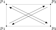
Example 10.1 (Reflections and translations).
Fix a rectangle in the euclidean plane with horizontal and vertical sides and label its corners as in Figure 5. Next, consider the group generated by the following eight elements: the four reflections that fix one of the four sides and the four translations that send a corner of this rectangle to the opposite corner. The reflection fixing and is denoted and the translation sending to is . Note that the subscripts of are unordered and the subscripts of are ordered. In this notation and are reflections fixing horizontal lines, and are reflections fixing vertical lines and the four translations are , , and . The group contains the isometry that rotates the rectangle about its center. For example, can be factored as . That this factorization is as short as possible over this generating set follows from the fact that every factorization must contain at least one horizontal reflection, one vertical reflection and one translation. In fact, it is straightforward to check that there are exactly such factorizations of length . The interval is shown in Figure 6. The dashed lines represent translations and the solid lines represent reflections with the thickness distinguishing horizontal and vertical reflections. Two final notes. The interval is not a lattice because there is a bowtie connecting the two leftmost vertices in each of the two middle rows. Concretely, the four factorizations of involved are , , and . And finally, these factorizations of form a single closed orbit under the Hurwitz action.

The -dimensional configuration described in Example 10.1 captures the essential reason why many of the intervals that define dual euclidean Artin groups fail to be lattices.
Proposition 10.2 (Bowties).
Let and be orthogonal reflections in an irreducible euclidean Coxeter group and let be a translation in in a root direction. If does not commute with either reflection and is not in the plane spanned by the roots of and , then the interval below the element contains a bowtie and is not a lattice.
Proof.
The first step is to show that the interval contains a copy of Figure 6 as an induced subposet. Because is a translation in a root direction it is a product of two parallel reflections in . This means that has reflection length at most . Next, note that is an elliptic element with a -dimensional move-set spanned by the roots of and . The hypothesis that does not lie in means that the move-set of is not through the origin and thus is a nonlinear -dimensional affine subspace. Thus is a hyperbolic isometry with reflection length at least . Combining these facts shows that and, after factoring into two parallel reflections in , we have one of its minimal length factorizations and a corresponding maximal chain in .
Next, let be any -dimensional affine subset of the euclidean space with and note that the hyperplanes fixed by the reflections and intersect in orthogonal lines and and that both and stabilize . If we uniquely decompose as a vector in plus a vector in then we can factor into a pair of translations and , one with a translation direction in and one with a translation direction in . The translation commutes with , and and the hypotheses on ensure that is nontrivial and not a direction vector of or . In particular, the way , and act on can be esssentially identified with the action of , and of Example 10.1.
As we use the Hurwitz orbit in the example to alter the factorization there, we can mimic that action on the minimal length reflection factorizations of , treating the translation as a product of two parallel reflections that always stay together and where both get conjugated simultaneously when necessary. Under this action, the translation simply follows the conjugates of the translation around by virtue of the fact that it commutes with all three actions on . The result is a copy of Figure 6 as an induced subposet of . The final step is to note that the bowtie visible on the left of Figure 6 remains a bowtie in the larger poset because is, in turn, an induced subposet of the hyperbolic poset where these same four elements, two of rank and two of rank are four elements forming one of the known bowties in as described in Theorem 5.5. ∎
Translations and reflections satisfying the hypotheses of Proposition 10.2 can be found below a Coxeter element in an irreducible euclidean Coxeter group whenever the roots orthogonal to the direction of its Coxeter axis form a reducible root system.
Theorem 10.3 (Reducibility and bowties).
Let be the axis of a Coxeter element in an irreducible euclidean Coxeter group . If the root system of horizontal roots is reducible, then the interval contains a bowtie, it is not a lattice and the dual Artin group is not a Garside group.
Proof.
Let be a chamber where the reflections defined by its facets can be multiplied in an appropriate order to produce . By repeatedly applying Lemma 7.4 and replacing with another chamber if necessary, we may assume without loss of generality that the reflection corresponding to the white dot is the reflection . When this is the case, the remaining reflections in the factorization fix a vertex of with the property that every hyperplane of a reflection in is parallel to a hyperplane of a reflection in fixing . In other words, we can identify as our origin as in Definition 6.4, the group generated by through is the group , and the product is a Coxeter element for . Because every reflection through occurs in some minimal length factorization of this Coxeter element, we may modify the product so that is a reflection with a hyperplane parallel to the hyperplane of . As a consequence is a translation in a root direction and concretely a translation in the direction that is the root of highest weight relative to this simple system.
Next, consider the element . This is an elliptic element fixing a line and since it differs from by a translation, is parallel to , the Coxeter axis of . Moreover, must lie in the hyperplane fixed by for each , so the roots of these reflections belong to the root system . We should note that the common root of and is not in this root system because they are now the only roots capable of moving points in a direction that includes motion in the direction of .
By hypothesis this system of horizontal roots is reducible, say for some with each an irreducible root system that spans a subspace and is an orthogonal decomposition of . Because the reflections , form a minimal length factorization of an elliptic isometry, their roots are linearly independent [BM, Lemma ]. Thus the number of roots in each is bounded above by the dimension of the corresponding . Moreover, since the number of reflections equals the dimension of , the roots of these reflections that lie in each form a basis for .
Finally, note that because the reflections generate all of , their roots must generate the entire irreducible root system . In partiuclar, the vector is not in for any since this would lead to an obvious decomposition. More to the point, there must be an with a root in is not orthogonal to since these roots form a basis of , and the same is true for the other components as well. In particular, we can select two reflections from our given factorization of with roots from distinct irreducible components of the horizontal root system and that neither one commutes with the translation and by Lemma 3.7 we may assume that they are and . At this point, we can apply Proposition 10.2 with , and to conclude that the interval from to contains a bowtie . But this interval is contained inside and the additional elements cannot resolve the bowtie since any element below and was already contained in . Thus contains a bowtie and is not a lattice. ∎
Consider the case of the Coxeter group. By comparing Figures 3 and 4 it is clear that there are exactly horizontal roots forming a root system. Since this is irreducible, Theorem 10.3 does not apply. This is consistent with Theorem 9.7 where we showed that the interval used to define the dual presentation of is a lattice and thus the dual presentation is a Garside presentation.
11. Computations and remarks
In this final section we use Theorem 10.3 to complete the proof of our main theorem, Theorem A. At this point it is relatively straightforward. For each type and representative Coxeter element we compute the direction of the Coxeter axis using Remark 8.4 and then we compute the system of horizontal roots. In each case not covered by [Dig06], [Dig12], or Theorem 9.7, the system of horizontal roots is reducible. We begin by introducing the relevant root systems using a slightly idiosyncratic notation that John Crisp and I have found to be quite useful when performing explicit root computations by hand.
Definition 11.1 (Root notation).
In almost every standard root system for a euclidean Coxeter group, a root is completely specified by indicating the location and the sign of its nonzero entries. This is because all nonzero entries has the same absolute value and this common value only depends on the number of nonzero entries. We list the locations of the nonzero entries in the subscript together with a slash “/”. The locations of the positive entries occur before the slash and the locations of the negative entries occur afterwards. For example, , and denote the vectors , and , respectively and in the root system the vector is written .
Definition 11.2 (Root systems).
Let be the collection of vectors of the form:
and let be the subset of these vectors with an even number of minus signs. The standard root systems of types , , , and are very easy to describe using this notation. See Table 1. The others involve slight modifications. The roots in that are orthogonal to the vector , i.e. the vector with all coordinates equal to , form the standard root system. The roots in orthogonal to , i.e. the roots with , form the standard root system. And the roots in orthogonal to and , i.e. the roots with , form the standard root system.
| Type | Roots |
|---|---|
We begin with the four classical families. The computations for type are done in greater detail because they are straightforward and indicate the kinds of computations that are merely sketched for the remaining types.
Example 11.3 (Type ).
We begin by selecting vectors from the root system whose nonpositive dot products are encoded in the diagram of Figure 2. From left to right we use , , , … and . In the notation of Definition 11.1 these are the vectors , and . Our choice of vectors is nonstandard, but it has the advantage of producing a bipartite Coxeter element whose axis is in a direction that makes computing and identifying the horizontal root system trivial. We compute the direction of the Coxeter axis following the procedure outlined in Remark 8.4. The unique linear dependency among these vectors involves adding the first and last vectors to two times each of the remaining vectors. The bipartite structure separates them based on parity in the list and the sum of the odd terms is the vector , or in Conway’s shorthand notation. The roots orthogonal to this direction are those of the form and these form the irreducile root system . Note that Theorem 10.3 is not applicable and that this is consistent with the results in [Dig12] where Digne established that the interval that defines the dual euclidean Artin group of type is, in fact, a lattice and the dual presentation of is a Garside presentation.
Type is very similar but has a reducible horizontal root system.
Example 11.4 (Type ).
Next consider the root system of type and select the vectors , , , …, , and to represent the vertices of the diagram of Figure 2 from left to right. In shorthand notation, these are the vectors , , , …, and , keeping in mind that denotes the vector in the root system and not as in the root system. The unique linear dependency among these vectors is obtained by adding the two final vectors to two times each of the remaining vectors. In , for example, the linear dependency is . Separating the terms based on the bipartite structure shows that the direction of the Coxeter axis is . The horizontal roots are those of the form with and the two roots . This is clearly a reducible horizontal root system with the components isomorphic to and . In particular, Theorem 10.3 applies, the interval used to define the dual euclidean Artin group of type is not a lattice and the dual presentation of is not a Garside presentation.
Type is another slight variation.
Example 11.5 (Type ).
Consider the root system of type and select the vectors , , , …, , and to represent the vertices of the diagram of Figure 2 from left to right. The unique linear dependency among these vectors is obtained by adding the first two vectors, the last two vectors, and two times each of the remaining vectors. In , for example, the linear dependency is . Separating the terms based on the bipartite structure shows that the direction of the Coxeter axis is . The horizontal roots are those of the form with and the four roots and This is a reducible horizontal root system with three irreducible factors (since and are orthogonal) that are isomorphic to , and . In particular, Theorem 10.3 applies, the interval used to define the dual euclidean Artin group of type is not a lattice and the dual presentation of is not a Garside presentation.
The final classical family is type .
Example 11.6 (Type ).
Let be the Coxeter group . For each with and we can construct a -bigon Coxeter element as follows. First let act on in the natural way, permuting coordinates and translating along vectors orthogonal to . Next label these coordinates . Let the unique source in the acyclic orientation be the reflection that swaps coordinates and , let the vertices along one side of the bigon represent reflections that swap and in ascending order and let the vertices along the other side represent reflections that swap and in ascending order. Finally, let the unique sink represent the reflection that sends the coordinates to . This is a reflection fixing the hyperplane . The product of these reflections in this order is an isometry of that sends to . Although we cannot use the method of Remark 8.4 to calculate the direction of the Coxeter axis, it is easy enough to compute that its -th power of this motion is a pure translation in the direction , i.e. the vector with its first coordinates equal to and its next coordinates equal to . Thus this is the direction of the axis of this Coxeter element.
As a consequence, the horizontal roots are those of the form with or with . So long as (and therefore ) is at least , there is at least one horizontal root of each type and the horizontal root system is reducible with one component isomorphic to a and the other component isomorphic to a . In particular, Theorem 10.3 applies to any -bigon Coxeter element with , the interval used to define the dual euclidean Artin group of type with respect to this Coxeter element is not a lattice and the corresponding dual presentation of is not a Garside presentation. In the remaining case where and , the horizontal roots for an irreducible root system and Theorem 10.3 is not applicable. This is consistent with the results in [Dig06] where Digne established that the interval that defines the dual euclidean Artin group of type with respect to an -bigon Coxeter element is, in fact, a lattice and the corresponding dual presentation is a Garside presentation.
And finally we shift our attention to the exceptional types. Since type is covered by Theorem 9.7, we only need to discuss the four remaining examples. In each case we list the vectors chosen to as our simple system, the resulting direction of the Coxeter axis and the vectors of the horizontal root system grouped into irreducible components. These computations were initially carried out by hand and then a few lines of code in GAP were used to doublecheck and validate these results.
Example 11.7 (Type ).
Consider the root system of type . If we select the vectors , , , , and from the root system as the vectors represented in the extended Dynkin diagram of type , then the direction of the axis of the corresponding bipartite Coxeter element is . There are roots that are horizontal with respect to this axis and they split into two irreducible factors. There is a root system formed by the roots and a root system formed by the roots . As a consequence Theorem 10.3 applies, the interval used to define the dual euclidean Artin group of type is not a lattice and the dual presentation of is not a Garside presentation.
Example 11.8 (Type ).
Consider the root system of type . If we select the vectors , , , , , and from the root system as the vectors represented in the extended Dynkin diagram of type , then the direction of the axis of the corresponding bipartite Coxeter element is . There are roots that are horizontal with respect to this axis and they split into three irreducible factors. There is a root system formed by the roots , another root system formed by the roots , and a root system formed by the roots .
Next consider the root system of type . If we select the vectors , , , , , , and from the root system as the vectors represented in the extended Dynkin diagram of type , then the direction of the axis of the corresponding bipartite Coxeter element is . There are roots that are horizontal with respect to this axis and they split into three irreducible factors. There is a root system formed by the roots , a root system formed by the roots , and a root system formed by the roots .
Finally consider the root system of type . If we select the vectors , , , , , , , and from the root system as the vectors represented in the extended Dynkin diagram of type , then the direction of the axis of the corresponding bipartite Coxeter element is . There are roots that are horizontal with respect to this axis and they split into three irreducible factors. There is a root system formed by the roots , , , , , , , , , and their negatives, a root system formed by the roots and a root system formed by the roots .
In each case, Theorem 10.3 applies, the interval used to define the dual euclidean Artin group of type for , or is not a lattice and the dual presentation of is not a Garside presentation.
At this point we have shown that for each type and for each geometric equivalence class of Coxeter elements not covered by earlier results, the resulting interval is not a lattice and the corresponding dual presentation is not a Garside presentation. This completes the proof of Theorem A. As a final comment we note that the existence of a uniform reason for the failure of the lattice property in all of these cases (i.e. reducibility of the horizontal root system) leads one to hope for the existence of a uniform way to work around the problem. This indeed turns out to be the case as Robert Sulway and I show in [MS] where we clarifying the basic structural properties of all euclidean Artin groups.
References
- [BDSW] Barbara Baumeister, Matthew Dyer, Christian Stump, and Patrick Wegener, A note on the transitive Hurwitz action on decompositions of parabolic Coxeter elements, arXiv:1402.2500 [math.GR].
- [Bes] David Bessis, Topology of complex reflection arrangements, Available at arXiv:math.GT/0411645.
- [Bes03] by same author, The dual braid monoid, Ann. Sci. École Norm. Sup. (4) 36 (2003), no. 5, 647–683. MR MR2032983 (2004m:20071)
- [BH99] Martin R. Bridson and André Haefliger, Metric spaces of non-positive curvature, Grundlehren der Mathematischen Wissenschaften [Fundamental Principles of Mathematical Sciences], vol. 319, Springer-Verlag, Berlin, 1999. MR 2000k:53038
- [BM] Noel Brady and Jon McCammond, Factoring euclidean isometries, To appear in the International Journal of Algebra and Computation arXiv:1312.7780.
- [BM00] Thomas Brady and Jonathan P. McCammond, Three-generator Artin groups of large type are biautomatic, J. Pure Appl. Algebra 151 (2000), no. 1, 1–9. MR 2001f:20076
- [BM10] Tom Brady and Jon McCammond, Braids, posets and orthoschemes, Algebr. Geom. Topol. 10 (2010), no. 4, 2277–2314.
- [CB92] William Crawley-Boevey, Exceptional sequences of representations of quivers, Proceedings of the Sixth International Conference on Representations of Algebras (Ottawa, ON, 1992) (Ottawa, ON), Carleton-Ottawa Math. Lecture Note Ser., vol. 14, Carleton Univ., 1992, p. 7. MR 1206935 (94c:16017)
- [CMW04] R. Charney, J. Meier, and K. Whittlesey, Bestvina’s normal form complex and the homology of Garside groups, Geom. Dedicata 105 (2004), 171–188. MR MR2057250 (2005e:20057)
- [DDG+] Patrick Dehornoy, François Digne, Eddy Godelle, Daan Krammer, and Jean Michel, Foundations of garside theory, arXiv:1309.0796.
- [DDM13] Patrick Dehornoy, François Digne, and Jean Michel, Garside families and Garside germs, J. Algebra 380 (2013), 109–145. MR 3023229
- [Dig06] F. Digne, Présentations duales des groupes de tresses de type affine , Comment. Math. Helv. 81 (2006), no. 1, 23–47. MR 2208796 (2006k:20075)
- [Dig12] by same author, A Garside presentation for Artin-Tits groups of type , Ann. Inst. Fourier (Grenoble) 62 (2012), no. 2, 641–666. MR 2985512
- [DP99] Patrick Dehornoy and Luis Paris, Gaussian groups and Garside groups, two generalisations of Artin groups, Proc. London Math. Soc. (3) 79 (1999), no. 3, 569–604. MR 2001f:20061
- [DP02] B. A. Davey and H. A. Priestley, Introduction to lattices and order, second ed., Cambridge University Press, New York, 2002. MR MR1902334 (2003e:06001)
- [Hum90] James E. Humphreys, Reflection groups and Coxeter groups, Cambridge Studies in Advanced Mathematics, vol. 29, Cambridge University Press, Cambridge, 1990. MR 1066460 (92h:20002)
- [Igu11] Kiyoshi Igusa, Exceptional sequences, braid groups and clusters, Groups, algebras and applications, Contemp. Math., vol. 537, Amer. Math. Soc., Providence, RI, 2011, pp. 227–240. MR 2799103 (2012f:16001)
- [IS10] Kiyoshi Igusa and Ralf Schiffler, Exceptional sequences and clusters, J. Algebra 323 (2010), no. 8, 2183–2202. MR 2596373 (2011b:20118)
- [IT09] Colin Ingalls and Hugh Thomas, Noncrossing partitions and representations of quivers, Compos. Math. 145 (2009), no. 6, 1533–1562. MR 2575093 (2010m:16021)
- [McCa] Jon McCammond, Pulling apart orthogonal groups to find continuous braids, Preprint 2010.
- [McCb] by same author, The structure of euclidean Artin groups, To appear in the Proceedings of the 2013 Durham conference on Geometric and Cohomological group theory arXiv:1312.7781.
- [MP11] Jon McCammond and T. Kyle Petersen, Bounding reflection length in an affine Coxeter group, J. Algebraic Combin. 34 (2011), no. 4, 711–719. MR 2842917 (2012h:20089)
- [MS] Jon McCammond and Robert Sulway, Artin groups of euclidean type, arXiv:1312.7770.
- [Rin94] Claus Michael Ringel, The braid group action on the set of exceptional sequences of a hereditary Artin algebra, Abelian group theory and related topics (Oberwolfach, 1993), Contemp. Math., vol. 171, Amer. Math. Soc., Providence, RI, 1994, pp. 339–352. MR 1293154 (95m:16006)
- [Squ87] Craig C. Squier, On certain -generator Artin groups, Trans. Amer. Math. Soc. 302 (1987), no. 1, 117–124. MR 887500 (88g:20069)
- [ST89] Ernst Snapper and Robert J. Troyer, Metric affine geometry, second ed., Dover Books on Advanced Mathematics, Dover Publications Inc., New York, 1989. MR 1034484 (90j:51001)
- [Sta97] Richard P. Stanley, Enumerative combinatorics. Vol. 1, Cambridge Studies in Advanced Mathematics, vol. 49, Cambridge University Press, Cambridge, 1997, With a foreword by Gian-Carlo Rota, Corrected reprint of the 1986 original. MR 98a:05001