Fermion Scattering in a Gravitational Background:

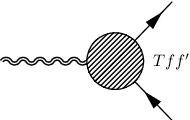
Radiative corrections to the graviton/matter vertex have been investigated since the 70’ s by Berends and Gastmans [1] in the QED case, who quantified the impact of these corrections to the bending of photons and fermions in an external localized gravitational field. These results were based on the study of 3-point functions (gravitational form factors) with two fermions ($Tff$) or two photons ($TVV$) in external gravity, and one insertion of the energy momentum tensor (EMT) $(T)$ of the matter fields.

The very small size of these corrections, which affect the angles of deflection, combined with the experimental difficulty to improve on their direct measurements, call into question the possibility of using these effects as a possible test of General Relativity. Perhaps, it is for this reason that the study of the electroweak corrections to the bending angles have not drawn any attention on these processes until the analysis of [2] and, more recently, of [3, 4], which concern the fermion/graviton vertex.

In the photon case, the $TVV$ vertex in QED has been re-investigated in the analysis of the conformal anomaly action in [5, 6], later extended to the electroweak case in [7, 8]. In the $Tff$ case, the study has been separated into the flavour-changing [2, 4] and flavour diagonal sectors [3], the first of the two playing a significant role in the analysis of possible flavour transitions in the presence of a scalar component in the external gravitational field, as pointed out in [2]. This aspect will be re-addressed in our current study.

The issue concerning the size of these corrections and their relevance can be resolved by noticing that the very same interactions become significant in the presence of sizeable gravitational backgrounds. Such are those due to black holes, which are ubiquitous in galactic centers, and surging to remarkable relevance in the analysis of galaxy structure formation. Obviously our formalism, which simply extends to the electroweak case the original analysis of [1], remains valid only in the case of small fluctuations around a flat spacetime metric, where curvature effects are ignored, and does not allow to handle backgrounds characterized by a strong curvature. It could, however, be extended to include further corrections related to the curvature scale of certain backgrounds, in the limit in which gravity is treated as an external classical source.

For this reason, we think that our analysis allows to highlight some of the basic features of the interaction of the Standard Model Lagrangian, once this is immersed in a weak gravitational background, clarifying some of the specific features of this coupling at a perturbative level. In particular, the renormalizability of the theory, which remains intact in this extended framework, is an important feature of these computations, not shared by other backgrounds.

One of the specific features of our results is their possible application to the neutrino sector, which has received some attention in recent years (see for instance [9, 10, 11]). We will provide indeed the expression for the QED and electroweak corrections to the scattering of a neutrino off an external source. These results are the starting point in the derivation of the equation relating the angle of deflection to the impact parameter of the collision, in the case of a static heavy source of the gravitational field. The use of an impact parameter formalism allows to merge the usual quantum corrections, computed in the exact electroweak theory, with the semiclassical method in which the incoming asymptotic quantum state is described by a particle approaching the source at a distance $b$, with $b$ denoting the impact parameter. This method has been used in [1] and in the more recent literature on the computation of corrections to the gravitational scattering of quantum fields both in static [12, 13] and in rotating (Lense-Thirring) backgrounds [14]. Except for the case of the QED corrections, already discussed in [1] and that we recompute, a general analysis of the weak corrections and of the modified lense equations, which may impact the structure of cosmic shears, is left to future work.

The primary goal of our work is to extend our previous analysis of the $Tff$ vertex, by computing the radiative corrections to the cross section in an external gravitational field, in the limit of a source of large mass, i.e. in a scattering off a potential. In this case we discuss both the limits of low and high momentum transfers. At low momentum transfers we derive an effective Hamiltonian which describes the flavour-changing transitions. We also discuss the cross section for the exchange of a scalar component for the gravitational field, with the inclusion of the electroweak effects. Our expressions for fermion scattering are specialized both to ordinary and to weakly interacting fermions, such as neutrinos or dark matter particles, by the inclusion of suitable form factors which account for interactions in the inner core of the source. We conclude our analysis with some perspectives and possible extensions of our work, to be left for further studies. Being this work the third in a sequel [3, 4], most of our previous notations and results will be necessary in order to proceed with the applications discussed here.

In this section we briefly review the main features of the coupling of the Standard Model in an external gravitational field, focusing our attention on the fermion sector. We recall that the dynamics of the Standard Model plus gravity is described by the action

$$\mathcal{S}=\mathcal{S}_{SM}+\mathcal{S}_{G}+\mathcal{S}_{I}$$

(1)

with $\mathcal{S}_{SM}$ containing the Standard Model (SM) Lagrangian, while

	$\displaystyle\mathcal{S}_{G}$	$\displaystyle=$	$\displaystyle-\frac{1}{\kappa^{2}}\int d^{4}x\sqrt{-{g}}\,R$
	$\displaystyle\mathcal{S}_{I}$	$\displaystyle=$	$\displaystyle\chi\int d^{4}x\sqrt{-{g}}\,R\,H^{\dagger}H$		(2)

denote respectively the Einstein gravitational term of the action and a term of improved action $\mathcal{S}_{I}$, involving the Higgs doublet $H$. The latter is responsible for generating a symmetric and traceless energy-momentum tensor (EMT) [15]. $\mathcal{S}_{SM}$ is obtained by extending the ordinary Lagrangian of the Standard Model to a curved metric background. $\mathcal{S}_{I}$ vanishes in the flat space time limit, due to the vanishing of the Ricci scalar in the same limit. Its corresponding EMT $(T_{I\,\mu\nu}$), however, is non-vanishing. With the inclusion of $\mathcal{S}_{I}$, varying the action $\mathcal{S}$ with respect to the fields of the SM allows to generate an EMT which is symmetric without any additional symmetrization. We remark that $\chi$ is conformal at the value $\chi\equiv\chi_{c}=1/6$ and guarantees the renormalizability of the model, including all Green functions at any order in $k$ containing only insertions of external graviton fields $h$, with $\kappa^{2}=16\pi G$.

We will be using the flat metric $\eta_{\mu\nu}=\textrm{diag}(1,-1,-1,-1)$, with an expansion of the form

	$\displaystyle g_{\mu\nu}=\eta_{\mu\nu}+\kappa h_{\mu\nu}+O(\kappa^{2})$
	$\displaystyle g^{\mu\nu}=\eta^{\mu\nu}-\kappa h^{\mu\nu}+O(\kappa^{2})$
	$\displaystyle\sqrt{-g}=1+\frac{\kappa}{2}h+O(\kappa^{2}),$		(3)

where $h\equiv h^{\mu\nu}\eta_{\mu\nu}$ is the trace of the metric fluctuations.

The interaction between the gravitational field and matter, at this order, is mediated by diagrams containing a single power of the EMT $T^{\mu\nu}$ and multiple fields of the Standard Model. The tree level coupling is summarized by the action

$$\mathcal{S}_{int}=-\frac{\kappa}{2}\int d^{4}x\,T_{\mu\nu}h^{\mu\nu}\,,$$

(4)

where $T_{\mu\nu}$ denotes the symmetric and covariantly conserved EMT of the Standard Model Lagrangian, embedded in a curved space-time background and defined as

$$T_{\mu\nu}=\frac{2}{\sqrt{-g}}\frac{\delta\left(S_{SM}+S_{I}\right)}{\delta g^{\mu\nu}}\bigg|_{g=\eta}\,.$$

(5)

The complete EMT of the Standard Model, including ghost and gauge-fixing contributions can be found in [8]. The fermionic part of the EMT is obtained using the vielbein formalism. Indeed the fermions are coupled to gravity by using the spin connection $\Omega$ induced by the curved metric $g_{\mu\nu}$. This allows the introduction of a derivative $\mathcal{D}_{\mu}$ which is covariant both under gauge and diffeomorphism transformations. Generically, the Lagrangian for a fermion $(f)$ takes the form

$\displaystyle\mathcal{L}_{F}=\sqrt{-g}\left(\frac{i}{2}\bar{\psi}\gamma^{\mu}(\mathcal{D}_{\mu}\psi)-\frac{i}{2}(\mathcal{D}_{\mu}\bar{\psi})\gamma^{\mu}\psi-m\,\bar{\psi}\psi\right)\,,$

(6)

where the covariant derivative is defined as $\mathcal{D}_{\mu}=\partial_{\mu}+A_{\mu}+\Omega_{\mu}$, with $A_{\mu}$ denoting the gauge field. The spin connection takes the form

$\displaystyle\Omega_{\mu}=\frac{1}{2}\sigma^{ab}V_{a}^{\nu}V_{b\nu;\mu}$

(7)

where $V$ is the vielbein, the semicolon denotes the gravitationally covariant derivative and $\sigma^{ab}$ are the generators of the Lorentz group in the spinorial representation. The latin indices are Lorentz indices of a local free-falling frame. The connection can be expanded as

$$\Omega_{\mu}=\frac{1}{4}\sigma^{mn}\left[V^{\nu}_{m}\left(\partial_{\mu}V_{n\nu}-\partial_{\nu}V_{n\mu}\right)+\frac{1}{2}V^{\rho}_{m}V^{\sigma}_{n}\left(\partial_{\sigma}V_{l\rho}-\partial_{\rho}V_{l\sigma}\right)V_{\mu}^{l}-(m\leftrightarrow n)\right].$$

(8)

with

$$V_{\mu}^{m}=\delta_{\mu}^{m}+\frac{\kappa}{2}h^{m}_{\mu}+O(\kappa^{2}).$$

(9)

At leading order the interacting Dirac Lagrangian (6) generates the terms

$\displaystyle\mathcal{L}_{F}$

$\displaystyle=$

$\displaystyle\mathcal{L}_{0}-\frac{\kappa}{2}h_{\mu\nu}T^{(0)\mu\nu}$

(10)

with $\mathcal{L}_{0}$ denoting the free Dirac term

$$\mathcal{L}_{0}=\frac{i}{2}\left(\bar{\psi}\stackrel{{\scriptstyle\rightarrow}}{{\not{\partial}}}\psi-\bar{\psi}\stackrel{{\scriptstyle\leftarrow}}{{\not{\partial}}}\psi\right)-m\bar{\psi}\psi$$

(11)

and the EMT of a Dirac fermion of mass $m_{f}$

$$T^{(0)}_{\mu\nu}=\frac{i}{4}\left((\bar{\psi}\gamma_{\mu}\partial_{\nu}\psi-\partial_{\nu}\bar{\psi}\gamma_{\mu}\psi)+(\mu\leftrightarrow\nu)\right)-\eta_{\mu\nu}\mathcal{L}_{0}$$

(12)

that we couple to the external field $h^{ext}_{\mu\nu}$. In momentum space the corresponding vertex takes the form (see Fig. 124)

$$V^{(0)\mu\nu}=\frac{i}{4}\left(\gamma^{\mu}(p_{1}+p_{2})^{\nu}+\gamma^{\nu}(p_{1}+p_{2})^{\mu}-2\eta^{\mu\nu}(\not{p}_{1}+\not{p}_{2}-2m)\right),$$

(13)

from which we have omitted an overall factor $(-\kappa/2)$ coming from the interaction Lagrangian, which will be reinserted at the level of the transition amplitude. Only diagonal transition amplitudes in flavour space are induced at leading order, while the inclusion of the electroweak corrections allows flavour-changing transitions, which will play a key role in our analysis.

We will denote with $\hat{T}^{\mu\nu}$ the transition amplitude between the intial and the final state induced by the insertions of the EMT vertex, with initial and final wave functions included, while $V^{\mu\nu}$ will be denoting the corresponding vertex in momentum space, i.e.

$$\hat{T}^{\mu\nu}=\bar{u}(p_{2})V^{\mu\nu}u(p_{1}),$$

(14)

having labeled the momenta of the incoming and outgoing fermion with $p_{1}$ and $p_{2}$ respectively. We will similarly use the notation

$$\hat{O}\equiv\bar{u}(p_{2})Ou(p_{1})$$

(15)

to denote the matrix element of any operator $O$ in momentum space. Using these notations, the same matrix element can be expressed in position space in terms of the operator $T^{\mu\nu}(x)$, inserted on the Dirac eigenstates given by incoming ($\psi_{i}$) and outgoing ($\psi_{f}$) plane waves

$$\langle p_{2}|T^{\mu\nu}(x)|p_{1}\rangle=\bar{\psi_{f}}(p_{2})V^{\mu\nu}\psi_{i}(p_{1})e^{iq\cdot x},$$

(16)

where $q=p_{1}-p_{2}$ is the 4-momentum transfer. We have introduced plane waves given by

$$\psi_{i}(p_{1})={\mathcal{N}_{i}}u(p_{1}),\qquad\mathcal{N}_{i}=\sqrt{\frac{m_{1}}{E_{1}V_{l}}},\qquad\bar{u}(p_{1})u(p_{1})=1,$$

(17)

and similarly for $\psi_{f}$, while $V_{l}$ denotes a finite volume normalization of the two scattering states. The $E_{1}$ ($E_{2}$) and $m_{1}$ ($m_{2}$) are the energy and corresponding mass of the incoming (outgoing) particle respectively.

The scattering matrix element is then written as

$$i\mathcal{S}_{if}=-\frac{\kappa}{2}\int_{\mathcal{V}}d^{4}x\langle p_{2}|h_{\mu\nu}(x)T^{\mu\nu}(x)|p_{1}\rangle,$$

(18)

where ${\mathcal{V}}$ denotes the relevant region of integration and with the gravitational field being external, which gives

$\displaystyle\langle p_{2}|h_{\mu\nu}(x)T^{\mu\nu}(x)|p_{1}\rangle$

$\displaystyle=$

$\displaystyle h_{\mu\nu}(x)\bar{\psi}(p_{2})V^{\mu\nu}\psi(p_{1})e^{iq\cdot x}.$

(19)

The scattering amplitude which can be immediately expressed in momentum space as

	$\displaystyle i\mathcal{S}_{fi}$	$\displaystyle=$	$\displaystyle-\frac{\kappa}{2}h_{\mu\nu}(q)\bar{\psi}(p_{2})V^{\mu\nu}\psi(p_{1})$		(20)
		$\displaystyle=$	$\displaystyle-\frac{\kappa}{2}h_{\mu\nu}(q)\mathcal{N}_{i}\mathcal{N}_{f}\hat{T}^{\mu\nu}$

in terms of the gravitational fluctuations in momentum space $h_{\mu\nu}(q)$, defined as in (32).
For a static external field the energies of the incoming/outgoing fermions are conserved ($E_{1}=E_{2}\equiv E$) both in the flavour-diagonal and non-diagonal cases, as one can immediately realize from (31). It is obvious that the interaction region depends both on the type of scattering particle and on the geometry of the source. We will consider the potential scattering of a Dirac fermion off an external static source, which acts as a perturbation on the otherwise flat spacetime background. The source is characterized by an EMT $T^{ext}_{\mu\nu}$ and the fluctuations are determined by solving the linearized equations of General Relativity.

We start analyzing the flavour-conserving transitions at leading order. In the rest of the paper, for simplicity, we will omit the flavour index from each spinor, together with the explicit flavour dependence on the masses of the internal flavours, which appear at 1-loop order. The linearized equations take the form

$$\square\left(h_{\mu\nu}-\frac{1}{2}\eta_{\mu\nu}h\right)=-{\kappa}T^{ext}_{\mu\nu}$$

(21)

and can be rewritten as

$$\square h_{\mu\nu}={\kappa}S_{\mu\nu},\qquad S_{\mu\nu}=-\left(T^{ext}_{\mu\nu}-\frac{1}{2}\eta_{\mu\nu}T^{ext}\right),$$

(22)

where we have denoted with $T^{ext}$ the EMT trace of the external source. The external field is obtained by convoluting the static source with the retarded propagator

$$G_{R}(x,y)=\frac{1}{4\pi}\frac{\delta(x_{0}-|\vec{x}-\vec{y}|-y_{0})}{|\vec{x}-\vec{y}|}$$

(23)

normalized as

$$\square G_{R}(x,y)=\delta^{4}(x-y).$$

(24)

The solution of (22) takes the form

$$h^{ext}_{\mu\nu}(x)={\kappa}\int d^{4}yG_{R}(x,y)S_{\mu\nu}(y),$$

(25)

with the EMT of the external localized source

$$T^{ext}_{\mu\nu}=\frac{P_{\mu}P_{\nu}}{P_{0}}\delta^{3}(\vec{x}),$$

(26)

which for a particle of mass $M$ at rest at the origin with $P_{\mu}=(M,\vec{0}$) takes the form

$$T^{ext}_{\mu\nu}=M\delta^{0}_{\mu}\delta^{0}_{\nu}\delta^{3}(\vec{x}).$$

(27)

This gives

$$S_{\mu\nu}=\frac{M}{2}\bar{S}_{\mu\nu}\qquad\bar{S}_{\mu\nu}\equiv\eta_{\mu\nu}-2\delta^{0}_{\mu}\delta^{0}_{\nu}$$

(28)

and the field generated by a local (point-like, $L$) mass distribution has a typical $1/r$ $(r\equiv|\vec{x}|)$ behaviour

$\displaystyle h^{L}_{\mu\nu}(x)$

$\displaystyle=$

$\displaystyle\frac{2GM}{\kappa|\vec{x}|}\bar{S}_{\mu\nu}.$

(29)

The fluctuations are normalized in such a way that $h_{\mu\nu}$ has mass dimension 1, as an ordinary bosonic field, with $\kappa$ of mass dimension ${-1}$.

The Fourier transform of $h_{\mu\nu}$ in momentum space is given by

$\displaystyle h_{\mu\nu}(q_{0},\vec{q})$

$\displaystyle=$

$\displaystyle\int d^{4}xe^{iq\cdot x}h_{\mu\nu}(x)$

which for a static field reduces to the form

$$h_{\mu\nu}(q_{0},\vec{q})=2\pi\delta(q_{0})h_{\mu\nu}(\vec{q}),$$

(31)

with

$$h_{\mu\nu}(\vec{q})\equiv h_{0}(\vec{q})\bar{S}_{\mu\nu}$$

(32)

defined in terms of the scalar form factor which is related to the geometrical structure of the external source. In the case of a point-like source, we obtain

	$\displaystyle h_{\mu\nu}(q_{0},\vec{q})$	$\displaystyle=$	$\displaystyle 2\pi\delta(q_{0})\times\frac{2GM}{\kappa}\bar{S}_{\mu\nu}\int d^{3}\vec{x}\frac{e^{i\vec{q}\cdot\vec{x}}}{|\vec{x}|}$		(33)
		$\displaystyle=$	$\displaystyle 2\pi\delta(q_{0})\times\left(\frac{\kappa M}{2\vec{q}^{2}}\right)\bar{S}_{\mu\nu},$

which gives

$$h_{0}(\vec{q})\equiv\left(\frac{\kappa M}{2\vec{q}^{2}}\right),\qquad h_{\mu\nu}(\vec{q})\equiv\left(\frac{\kappa M}{2\vec{q}^{2}}\right)\bar{S}_{\mu\nu}.$$

(34)

At the same time, the leading order interaction is redefined as

$$V^{(0)\mu\nu}\equiv{i}O_{V}^{(0)\mu\nu},$$

(35)

with

$$O_{V}^{(0)\mu\nu}=\frac{1}{4}\left(p^{\mu}\gamma^{\nu}+p^{\nu}\gamma^{\mu}-2\eta^{\mu\nu}(\not{p}-2m)\right),$$

(36)

which will turn useful in the computation of the radiative corrections. Using the matrix element

$$\bar{\psi}_{f}(x)T^{(0)\mu\nu}\psi_{i}(x)=\left(-\frac{\kappa}{2}\right)\times\mathcal{N}_{i}\mathcal{N}_{f}\times i\bar{u}(p_{2})O_{V}^{(0)\mu\nu}u(p_{1})e^{iq\cdot x}$$

(37)

the leading order scattering amplitude can be rewritten as

	$\displaystyle i\mathcal{S}^{(0)}_{if}$	$\displaystyle=$	$\displaystyle\int d^{4}xh_{\mu\nu}(x)\bar{\psi}_{f}(x)T^{(0)\mu\nu}\psi_{i}(x)$		(38)
		$\displaystyle=$	$\displaystyle\left(-\frac{\kappa}{2}\right)\times\mathcal{N}_{i}\mathcal{N}_{f}\times\left(ih_{\mu\nu}(\vec{q})\bar{u}(p_{2})O_{V}^{(0)\mu\nu}u(p_{1})\right)\times 2\pi\delta(q_{0}).$

The averaged squared amplitude then takes the form

$\displaystyle\langle|i\mathcal{S}^{(0)}_{if}|^{2}\rangle$

$\displaystyle=$

$\displaystyle\left(-\frac{\kappa}{2}\right)^{2}\left(\mathcal{N}_{i}\mathcal{N}_{f}\right)^{2}\times\left(2\pi\delta(q_{0})\mathcal{T}\right)\times\left(\frac{\kappa M}{2\vec{q}^{2}}\right)^{2}\times\frac{1}{2}\mathcal{Y}_{0},$

(39)

where we have introduced a factor (1/2) for the fermion spin average. As usual, we have extracted, from the square of the delta function, the transition time $\mathcal{T}$, using $(2\pi\delta(q_{0}))^{2}=2\pi\delta(q_{0})\mathcal{T}$. We have defined

	$\displaystyle\mathcal{Y}_{0}$	$\displaystyle=$	$\displaystyle\frac{1}{4m^{2}}Tr\left[(\not{p}_{2}+m)O_{V}^{(0)\mu\nu}(\not{p}_{1}+m)O_{V}^{(0)\alpha\beta}\right]\bar{S}_{\mu\nu}\bar{S}_{\alpha\beta}$		(40)
		$\displaystyle=$	$\displaystyle E^{2}\textrm{Tr}\left[\frac{\not{p_{2}}+m}{2m}\left(2\gamma^{0}-\frac{m}{E}\right)\frac{\not{p_{1}}+m}{2m}\left(2\gamma^{0}-\frac{m}{E}\right)\right]$
		$\displaystyle=$	$\displaystyle 8\frac{\vec{p_{1}}^{4}}{m^{2}}F^{(0)}(x,\theta)$

in the flavour-diagonal case, with $F^{(0)}(x,\theta)$ given by

$$F^{(0)}(x,\theta)=\cos^{2}\frac{\theta}{2}+\frac{x}{4}+\frac{x^{2}}{4}+\frac{3}{4}{x}\cos^{2}\frac{\theta}{2},$$

(41)

with $x=m^{2}/\vec{p_{1}}^{2}$ and $\vec{p_{1}}$ the 3-momentum of the incoming fermion. We have used the relations $\vec{p}_{f}\equiv|\vec{p}_{1}|=|\vec{p}_{2}|$ in the elastic limit, while $\vec{q}^{\,2}=4\vec{p_{1}}^{\,2}\sin^{2}\theta/2$ and $q^{2}=-\vec{q}^{\,2}$.

To compute the differential cross section we define the transition probability from the initial state ($i$) into a set of final states ($f$) of differential $dn_{f}$ given by

$$dW=\frac{\vline\,i\mathcal{S}_{if}\,\vline^{2}}{j_{i}}dn_{f}$$

(42)

normalized with respect to the incident flux $j_{i}=\vec{p_{1}}/(E_{i}V)$ with the final state density, with a volume normalization $V$ given by

$$dn_{f}=\frac{V}{(2\pi)^{3}}d^{3}\vec{p}_{f}=\frac{V}{(2\pi)^{3}}|\vec{p_{2}}|E_{2}dE_{2}d\Omega,$$

(43)

which allows to define the cross section as the differential transition rate per unit time $(d\sigma\equiv{dW}/{\mathcal{T}})$. Combining all the contributions together and integrating over the energy of the final state we obtain

	$\displaystyle\frac{d\sigma}{d\Omega}$	$\displaystyle\equiv$	$\displaystyle\frac{d\sigma}{d\Omega}|_{L}$		(44)
		$\displaystyle=$	$\displaystyle\left(\frac{GM}{\sin^{2}\frac{\theta}{2}}\right)^{2}F^{(0)}(x,\theta).$

The result in Eq. (44) is in agreement with the corresponding one evaluated in Ref. [16]. In the following sections we will refer to this cross section as to the localized one, denoted in (44) also as $d\sigma/d\Omega|_{L}$, being generated by a gravitational point-like source located at the origin. This will turn useful in order to make a distinction between the cross sections of localized and of extended sources. The computation of the angle of deflection for the fermion involves a simple semiclassical analysis, in which one introduces the impact parameter representation of the same cross section. Assuming that the incoming particle is moving along the $z$ direction, with the source localized at the origin, and denoting with $\theta$ the azymuthal angle, we have the relation

$$\frac{b}{\sin\theta}\vline\frac{db}{d\theta}\vline=\frac{d\sigma}{d\Omega}$$

(45)

between the impact parameter $b$ and the scattering angle $\theta$, measured from the $z-$direction. This semiclassical approach allows to relate the quantum interaction between the particle and the source. We recall, if not obvious, that in the classical description the relation between $b$ and the deflection angle $\theta_{d}$ is obtained from energy and angular momentum conservation. In this respect Eq. (45) takes a similar role. The relation between $b$ and $\theta$ as a function of the incoming energy ($b=b(E,\theta)$), at least for small deflection angles, which correspond to large impact parameters, can be found analytically, but it should be integrated numerically otherwise. In the case of the point-like cross section $(L)$, for instance, one obtains the differential relation

$$\frac{db^{2}}{d\theta}=-2\left(\frac{GM}{\sin^{2}\frac{\theta}{2}}\right)^{2}F^{(0)}(x,\theta)\sin\theta$$

(46)

which gives

$$b^{2}(\theta)=(GM)^{2}\left(\frac{(2+x)^{2}}{\sin^{2}(\frac{\theta}{2})}+2(4+3x)\log\left(\sin(\frac{\theta}{2})\right)\right).$$

(47)

In the small $\theta$ limit we get the relations

$$b\sim GM\left(\frac{4}{\theta}+\frac{2x}{\theta}+(1+\frac{x}{4})\theta\log\theta\right)+{\cal O}(x^{2}\theta\log\theta)+{\cal O}(\theta),$$

(48)

which allows us to identify the deflection angle as

$$\theta\equiv\theta_{d}\sim 4\frac{GM}{b}.$$

(49)

Notice that in general $x\ll 1$ for a scattering at high energy, being the fermion mass small compared to the incoming energy or three-momentum. Onbviously, the bending angle of neutrinos, charged leptons and dark matter particles will be affected by the geometry of the source and by the strength of the fermion interaction with the source. This will vary if, for instance, the particles are allowed to enter the core of the gravitational source, as in the neutrino and the dark matter cases. For this reason we will proceed by determining the structure of these corrections, providing more general cross sections beyond the point-like approximation.

The one-loop corrections to the graviational fermion vertex in the framework of the SM, have been computed in Refs. [3] and [2, 4] for the flavor diagonal and off-diagonal transitions, for the case of external on-shell fermions. Exact results at one-loop order in all masses and momenta are provided for the corresponding form factors in Refs. [3] and [4].
The expression up to 1-loop order of the contributions to the fermion-fermion-graviton vertex $(ffg)$ can be organized in terms of a flavour-conserving (or diagonal) sector contribution and of a flavour-changing part. The diagonal sector receives contributions at tree level (i.e. from $\hat{T}^{(0)}_{\mu\nu}$), and at 1-loop from the virtual exchange of a photon ($\hat{T}_{\gamma}^{\mu\nu}$), a gluon ($\hat{T}_{g}^{\mu\nu}$), a $Z$ ($\hat{T}_{Z}^{\mu\nu}$) and a $W$, the latter denoted as $\hat{T}^{D\,\mu\nu}_{W}$. In the flavour-changing (non diagonal) sector the corrections start at 1-loop and are generated only from the exchange of a virtual $W$, denoted as $\hat{T}^{ND\,\mu\nu}_{W,{\bf ff^{\prime}}}$. As usual, the radiative corrections can be splitted into vertex corrections and the related counter-terms. We use the expression counter-terms to refer to the sum of those diagrams coming from the self-energy contributions to the external fermion legs, plus the corresponding diagrams coming from their wave-function renormalization. In the case of the flavor-changing transitions, the latter contributions are absent at one-loop level in the EMT counterterms, due to the fact that the fermion-graviton vertex is flavor-conserving at tree-level [2, 4]. Because of the energy momentum conservation, the radiative corrections induced by SM fields (no graviton loop corrections) to the EMT are finite at any order in perturbation theory, which implies the nonrenormalization of the Newton constant.

It is convenient to separate the diagonal ($D$) from the non-diagonal ($ND$) parts using the notation

$$T^{\,\mu\nu}_{\bf ff^{\prime}}=T^{D,\mu\nu}_{\bf ff^{\prime}}+T^{ND\,\mu\nu}_{\bf ff^{\prime}}$$

(61)

with $T^{D\,\mu\nu}_{\bf ff^{\prime}}$ expressed as

$$T^{D\,\mu\nu}_{\bf ff^{\prime}}=\delta_{\bf ff^{\prime}}T^{D\,\mu\nu},$$

(62)

where the flavour-conserving transitions are

$$\hat{T}^{D\,\mu\nu}=\hat{T}^{(0)}_{\mu\nu}+\hat{T}^{\mu\nu}_{g}+\hat{T}^{\mu\nu}_{\gamma}+\hat{T}^{\mu\nu}_{h}+\hat{T}^{\mu\nu}_{Z}$$

(63)

while the flavour-changing matrix elements take the form

$\displaystyle\hat{T}^{ND\,\mu\nu}_{\bf ff^{\prime}}=\hat{T}^{ND\,\mu\nu}_{W,\bf ff^{\prime}}$

(64)

since these can be generated only by the W exchange. The contributions given above are expanded in terms of a set of operators $O_{l}$ and intermediate form factors $F_{l}$, multiplied by the CKM matrix elements, related to internal the flavour transitions in the internal vertices of the diagrams. These are accounted for by the $V_{\bf fn}$ matrix elements, with the indices $\bf f$ and $\bf n$ corresponding to the flavour of the external and internal-loop fermions respectively. Generically, the flavour structure can be completely absorbed into some final form factors $f^{w}_{l}(q)$

$\displaystyle f^{w\,\bf{ff^{\prime}}}_{l}(q^{2})=\sum_{\bf n}V_{\bf fn}^{*}V_{\bf nf^{\prime}}\,F_{l}(q^{2},x_{f}),$

(65)

as we are going to specify below.
In the followings we will drop the flavour dependence on $f^{w}_{l}$, just to simplify the expressions, and the distinction between the (flavour) diagonal and non diagonal cases will be made evident by use of the superscript $ND$ (Non Diagonal) in the flavour-changing cases. In the diagonal case the contributions coming from the electromagnetic and weak transitions will be summarized by the form factors $f_{k}$, with $k=1\ldots 4$ and $(f^{h}_{l},f^{Z}_{l},f^{W}_{l},)$ with $l=1,\ldots 6$ respectively. In the non diagonal case, the $f^{ND}_{j}$, with $j=1,\ldots 12$, will completely describe all the corresponding transitions. The flavour structure will be omitted also from the EMT in both cases. We will also denote with $m_{f},m_{f^{\prime}}$ the masses of the initial and final state fermions. All the expressions of the form factors discussed in this work can be found in [2, 3, 4].

References

• [1] F. A. Berends and R. Gastmans, Ann. Phys. 98, 225 (1976).
• [2] G. Degrassi, E. Gabrielli, and L. Trentadue, Phys.Rev. D79, 053004 (2009), arXiv:0812.3262.
• [3] C. Corianò, L. Delle Rose, E. Gabrielli, and L. Trentadue, Phys.Rev. D87, 054020 (2013), arXiv:1212.5029.
• [4] C. Corianò, L. Delle Rose, E. Gabrielli, and L. Trentadue, Phys.Rev. D88, 085008 (2013), arXiv:1303.1305.
• [5] M. Giannotti and E. Mottola, Phys. Rev. D79, 045014 (2009), arXiv:0812.0351.
• [6] R. Armillis, C. Corianò, and L. Delle Rose, Phys. Rev. D81, 085001 (2010), arXiv:0910.3381.
• [7] C. Corianò, L. Delle Rose, A. Quintavalle, and M. Serino, Phys.Lett. B700, 29 (2011), arXiv:1101.1624.
• [8] C. Corianò, L. Delle Rose, and M. Serino, Phys.Rev. D83, 125028 (2011), arXiv:1102.4558.
• [9] R. Escribano, J. Frere, D. Monderen, and V. Van Elewyck, Phys.Lett. B512, 8 (2001), arXiv:hep-ph/0105211.
• [10] O. Mena, I. Mocioiu, and C. Quigg, Astropart.Phys. 28, 348 (2007), arXiv:astro-ph/0610918.
• [11] E. F. Eiroa and G. E. Romero, Phys.Lett. B663, 377 (2008), arXiv:0802.4251.
• [12] A. Accioly and R. Paszko, Phys.Rev. D69, 107501 (2004).
• [13] F. Sorge and S. Zilio, Class.Quant.Grav. 25, 225004 (2008).
• [14] F. Sorge, Class.Quant.Grav. 29, 045002 (2012).
• [15] J. Callan, Curtis G., S. R. Coleman, and R. Jackiw, Annals Phys. 59, 42 (1970).
• [16] J. Lawrence, Annals Phys. 58, 47 (1970).
• [17] G. Zatsepin and V. Kuzmin, JETP Lett. 4, 78 (1966).
• [18] K. Greisen, Phys.Rev.Lett. 16, 748 (1966).