Short random circuits define good quantum error correcting codes

We prove that random quantum circuits with $O(n\log^{2}n)$ gates can be used to encode $k$ qubits in $n$ qubits with a distance $d$ provided $\frac{k}{n}<1-\frac{d}{n}\log_{2}3-h(\frac{d}{n})$. This is asymptotically the same as the distance of a code defined by a random unitary from the complete Clifford group, which is known to achieve the quantum Gilbert-Varshamov bound [5, 12]. But a typical Clifford unitary is only known to be computable using a circuit with $\Omega(n^{2})$ gates.

We also study another complexity measure for circuits which is the depth. The depth is simply the number of time steps needed to evaluate the circuit, keeping in mind that gates acting on disjoint qubits can be executed simultaneously. By parallelizing the random quantum circuit mentioned in the previous paragraph, we prove the existence of codes achieving the same parameters with an encoding of depth $O(\log^{3}n)$ and size $O(n\log^{2}n)$. We remark that it was proved in [15] that the encoding and decoding operation of any stabilizer code can be implemented with quantum circuits of depth $O(\log n)$ using $O(n^{2})$ qubits of ancilla, i.e., qubits in some fixed state that are restored to their original state at the end of the computation. In contrast, random quantum circuits do not use any ancilla qubits.

We say here a brief word on the proof. The first step of the proof is to relate the property of interest, which is the distance of the code, to the second moment operator of the random quantum circuit. This operator can then be studied as a Markov chain and the distance of the code translates to a property of the Markov chain. The convergence times of such Markov chains arising from the second order moments have been previously studied in [17, 13]. However, these convergence times are not sufficient to prove the result we are aiming for and can only give useful bounds when $\Omega(n^{2})$ gates are applied. Instead, we analyze the Markov chain in a finer way without using the spectral gap and bound the probabilities of going from a state $\ell$ to state $m$ within $O(n\log^{2}n)$ steps as a function of $\ell$ and $m$.

The state of a pure quantum system is represented by a unit vector in a Hilbert space. Quantum systems are denoted $A,B,C\dots$ and are identified with their corresponding Hilbert spaces. The Hilbert spaces we consider here will be $n$-qubits spaces of the form $({{\mathbb{C}}}^{2})^{\otimes n}$. A density operator is a Hermitian positive semidefinite operator with unit trace. The density operator associated with a pure state is abbreviated by omitting the ket and bra $\psi\stackrel{{\scriptstyle\textrm{def}}}{{=}}|\psi\rangle\!\langle\psi|$. For an introduction to quantum information, we refer the reader to [16, 19].

Throughout the paper, we use the Pauli basis to decompose operators. The $2\times 2$ Pauli operators can be represented as follows:

$$\sigma_{0}=\left(\begin{array}[]{cc}1&0\\ 0&1\\ \end{array}\right)\qquad\sigma_{1}=\left(\begin{array}[]{cc}0&1\\ 1&0\\ \end{array}\right)$$

$$\sigma_{2}=\left(\begin{array}[]{cc}0&-i\\ i&0\\ \end{array}\right)\qquad\sigma_{3}=\left(\begin{array}[]{cc}1&0\\ 0&-1\\ \end{array}\right).$$

For a string $\nu\in\{0,1,2,3\}^{n}$, we define $\sigma_{\nu}=\sigma_{\nu_{1}}\otimes\cdots\otimes\sigma_{\nu_{n}}$. The support $\textrm{supp}(\nu)$ of $\nu$ is simply the subset $\{i\in[n]\mathrel{\mathop{\mathchar 58\relax}}\nu_{i}\neq 0\}$ and the weight $w(\nu)=|\textrm{supp}(\nu)|$. Any operator acting on $({{\mathbb{C}}}^{2})^{\otimes n}$ can be represented as

$$T=\frac{1}{2^{n}}\sum_{\nu\in\{0,1,2,3\}}\operatorname{tr}[\sigma_{\nu}T]\sigma_{\nu}.$$

As we are interested in the encoding complexity of quantum error correcting codes, we describe codes using the encoding operation. The encoding operation is a unitary transformation on an $n$-qubit space that we decompose as $A\otimes B$. It takes as input a $k$-qubit state $|\psi\rangle\in A$ (the state to be encoded) and the remaining input qubits are set to $|0\rangle^{\otimes n-k}\in B$. Such a code is called an $[n,k]$ quantum error correcting code. See Figure 1 for an illustration.

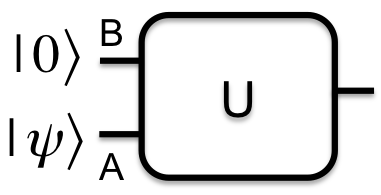
For an encoding unitary $U$, the code space is defined as the vector space $\{U|\psi\rangle|0\rangle^{\otimes n-k}\mathrel{\mathop{\mathchar 58\relax}}|\psi\rangle\in({{\mathbb{C}}}^{2})^{\otimes k}\}$. By considering a basis $\{|x\rangle\mathrel{\mathop{\mathchar 58\relax}}x\in\{0,1\}^{k}\}$ of $A$, we obtain a basis $\{|\bar{x}\rangle=U|x\rangle\otimes|0\rangle^{\otimes n-k}\mathrel{\mathop{\mathchar 58\relax}}x\in\{0,1\}^{n-k}\}$ of the code space. A code has distance at least $d+1$ if we have for all $x,y\in\{0,1\}^{k}$ and all $\mu\in\{0,1,2,3\}^{n}$ with $1\leq w(\mu)\leq d$

$$\langle\bar{x}|\sigma_{\mu}|\bar{y}\rangle=C_{\mu}\delta_{xy}$$

(1)

for some real numbers $C_{\mu}$ depending only on $\mu$ and not on $x,y$ [2, 14]. Here, $\delta_{xy}=1$ if $x=y$ and zero otherwise. A code with minimum distance $2e+1$ can correct $e$ errors.

We can describe a unitary transformation (and more generally any superoperator) by describing how it acts on the Pauli basis, i.e., $U\sigma_{\nu}U^{\dagger}$ for all $\nu\in\{0,1,2,3\}^{n}$. This is especially convenient when talking about stabilizer codes for which the encoding operation $U$ belongs to the Clifford group. The Clifford group ${\cal C}_{n}$ is defined as the set of unitary transformation $U$ under which the Pauli basis remains invariant up to phases. More precisely ${\cal C}_{n}=\left\{U\mathrel{\mathop{\mathchar 58\relax}}U\sigma_{\nu}U^{\dagger}\in\pm\{\sigma_{\mu},\mu\in\{0,1,2,3\}^{n}\}\right\}$. Note that any unitary in ${\cal C}_{n}$ can be implemented using Hadamard gates, phase gates and CNOT gates. When the encoding unitary $U\in{\cal C}_{n}$, the minimum distance can be simply characterized as shown by the following proposition.

We consider the following simple model for a quantum circuit acting on $n$ qubits. In a sequential random quantum circuit, a random two-qubit gate is applied to a randomly chosen pair of qubits in each time step. Here, the random two-qubit gate is going to be a random Clifford gate in ${\cal C}_{2}$ acting on two qubits.

A model of random circuits of a certain size defines a measure over unitary transformations on $n$ qubits that we call $p_{\textrm{circ}}$. The second-order moment operator will play an important role in all our proofs. The second-order moment operator is a superoperator acting on two copies of the space of operators acting on the ambient Hilbert space, which is an $n$-qubit space in our setting. For a measure $p$ over the unitary group, we can define the second moment operator $\operatorname{M}_{p}$ as

$$\operatorname{M}_{p}[X\otimes Y]=\underset{U\sim p}{\mathbf{E}}\left\{UXU^{\dagger}\otimes UYU^{\dagger}\right\}.$$

Even though we do not use the notion unitary designs here, it is worth pointing out that a distribution $p$ over unitary transformations is called a two-design if $\operatorname{M}_{p}=\operatorname{M}_{\textrm{clifford}}$ where clifford is the uniform distribution over the Clifford group [8]. We denote by $\operatorname{M}_{\textrm{circ}}$ the moment operator for the distribution obtained by applying one step of the random circuit. It is possible to compute $\operatorname{M}_{\textrm{circ}}$ explicitly when a random Clifford gate is applied to a randomly chosen pair $i,j$ of qubits, see e.g., [13, Section 3.2]. We have

$$\operatorname{M}_{\textrm{circ}}=\frac{1}{n(n-1)}\sum_{i\neq j}\operatorname{m}_{ij},$$

where $\operatorname{m}_{ij}$ only acts on qubits $i$ and $j$ and is defined by

$$\operatorname{m}_{ij}[\sigma_{\mu}\otimes\sigma_{\mu^{\prime}}]=\left\{\begin{array}[]{ll}0&\text{if }\mu\neq\mu^{\prime}\\ \sigma_{0}\otimes\sigma_{0}&\text{if }\mu=\mu^{\prime}=0\\ \frac{1}{15}\sum\limits_{\nu\in\{0,1,2,3\}^{2},\nu\neq 0}\sigma_{\nu}\otimes\sigma_{\nu}&\text{if }\mu=\mu^{\prime}\neq 0\\ \end{array}\right.$$

for all $\mu,\mu^{\prime}\in\{0,1,2,3\}^{2}$. We can thus represent the operator $\operatorname{M}_{\textrm{circ}}$ in the Pauli basis using the following $4^{n}\times 4^{n}$ matrix

$$Q(\mu,\nu)=\frac{1}{4^{n}}\operatorname{tr}\left[\sigma_{\nu}\otimes\sigma_{\nu}\operatorname{M}_{\textrm{circ}}[\sigma_{\mu}\otimes\sigma_{\mu}]\right].$$

In fact, it is simple to verify that $\sum_{\nu\in\{0,1,2,3\}^{n}}Q(\mu,\nu)=1$ for all $\mu$ and so $Q$ can be seen as a transition matrix for a Markov chain over the Pauli strings of length $n$.

Now for a random circuit with $t$ independent random gates applied sequentially, the second moment operator is simply $\operatorname{M}_{\textrm{circ}}^{t}$ and the corresponding matrix in the Pauli basis is also the $t$-th power of $Q$. The properties we are interested in can be expressed as quadratic functions of the entries of unitary transformation defined by the circuit and thus can be computed from the second moment operator. This means that these properties can be completely reduced to studying the evolution of the Markov chain defined by $Q$.

The objective of this section is to prove the main result of the paper: a typical circuit with $t=O(n\log^{2}n)$ gates defines an encoding into a quantum error correcting code with distance that is basically as good as for random Clifford unitaries. Let $h$ be the binary entropy function defined by $h(x)=-x\log_{2}x-(1-x)\log_{2}(1-x)$.

Let us state some remarks about this theorem. If instead of a random circuit, we were to apply a completely random Clifford unitary on $n$ qubits, we would have transition probabilities that are independent of $\ell$:

$$P_{\textrm{clifford}}(\ell,m)=\frac{\binom{n}{m}3^{m}}{4^{n}-1}.$$

Also the dependence in $\ell$ is close to optimal. Starting at state $\ell$, there is a probability of roughly $\frac{1}{3^{\ell}\binom{n}{\ell}}$ to get back to the state $1$. And in state $1$, there is a probability of $2^{-O(\log^{2}n)}$ of staying there for $t=O(n\log^{2}n)$ steps.

In order to bound expression (5), we first evaluate $\sum_{p=0}^{\ell}\binom{k}{p}3^{p}\binom{n-k}{\ell-p}$. We bound this sum simply by finding the $p$ for which it is maximum. In order to do so, note that the ratio

$$\frac{\binom{k}{p+1}3^{p+1}\binom{n-k}{\ell-p-1}}{\binom{k}{p}3^{p}\binom{n-k}{\ell-p}}=3\frac{(k-p)(\ell-p)}{(p+1)(n-k+p-\ell+1)}$$

is a decreasing function of $p$. Moreover, if we plug $p=\lambda\ell$ with $\lambda=\frac{3k}{n+2k}$ in this expression, we obtain

$$\frac{6k^{2}\ell-9k\ell^{2}+3k\ell n}{4k^{2}-2k\ell+6k^{2}\ell-3k\ell^{2}+4kn-\ell n+3k\ell n+n^{2}}\leq 1.$$

This means that the maximum occurs for some $p_{\max}\leq\left\lceil\lambda\ell\right\rceil$. As a result, we can bound the sum by

	$\displaystyle\sum_{p=0}^{\ell}\binom{k}{p}3^{p}\binom{n-k}{\ell-p}$	$\displaystyle\leq(\ell+1)\cdot 3^{p_{\max}}\binom{k}{p_{\max}}\binom{n-k}{\ell-p_{\max}}$
		$\displaystyle\leq(\ell+1)\cdot 3^{\lambda\ell+1}\sum_{p=0}^{\ell}\binom{k}{p}\binom{n-k}{\ell-p}$
		$\displaystyle=(\ell+1)\cdot 3^{\lambda\ell+1}\binom{n}{\ell}.$

Note that if $k>(1-\delta)n$, there is nothing to prove because the probability bound given by the theorem is negative. Assuming $k\leq(1-\delta)n$ and choosing $\eta$ appropriately small to apply Theorem III.2, we obtain

$$\sum_{p=0}^{\ell}\binom{k}{p}3^{p}\binom{n-k}{\ell-p}\frac{1}{(3-\eta)^{\ell}\binom{n}{\ell}}\frac{1}{n^{10}}\leq\frac{1}{n^{10}}.$$

Also observe that

$$\sum_{\ell=1}^{n}\sum_{p=0}^{\ell}\binom{k}{p}3^{p}\binom{n-k}{\ell-p}\leq 2^{n+k}-1.$$

Combining this with (7) and plugging this into (5), we obtain

		$\displaystyle\sum_{\ell=1}^{n}\sum_{p=0}^{\ell}\binom{k}{p}3^{p}\binom{n-k}{\ell-p}\sum_{m=1}^{d}P^{t}(\ell,m)$
		$\displaystyle\leq\sum_{\ell=1}^{n}\sum_{m=1}^{d}(2^{n+k}-1)\cdot 4^{\delta n}\cdot\frac{\binom{n}{m}3^{m}}{4^{n}-1}+\frac{1}{n^{10}}$
		$\displaystyle\leq\frac{1}{n^{8}}+n4^{\delta n}2^{k-n}\sum_{m=1}^{d}\binom{n}{m}3^{m}$
		$\displaystyle\leq\frac{1}{n^{8}}+2^{k-n\left(1-h(d/n)-\log_{2}(3)d/n-3\delta\right)}$		(8)

for sufficiently large $n$.   $\sqcap$$\sqcup$

In the previous section, the complexity measure for a circuit was the number of two-qubit gates applied. Another important complexity measure for circuits is the depth. The depth is related to the time complexity, or the number of time steps needed in order to execute the circuit. Note that two gates acting on disjoint qubits could in fact be executed simultaneously. For the problem of finding good error correcting codes, a natural question is how small can the depth of encoding circuits be. In this section, we show that by parallelizing the random quantum circuits considered in the previous section, we obtain with high probability circuits with depth $O(\log^{3}n)$. Using Theorem III.1, this proves that typical circuits of polylogarithmic depth define quantum error correcting codes that achieve a distance that is basically as good as the distance of a random stabilizer code.

To construct the parallelized circuit, one keeps adding gates to the current level until there is a gate that shares a qubit with a previously added gate in that level, in which case create a new level and continue. In the following proposition, we prove that by parallelizing a random circuit on $n$ qubits having $t$ gates we obtain with high probability a circuit of depth $O(\frac{t}{n}\log n)$.

References

- [1] L. Bazzi and S. Mitter, “Endcoding complexity versus minimum distance,” IEEE Trans. Inform. Theory, vol. 51, no. 6, pp. 2103–2112, 2005.
- [2] C. H. Bennett, D. DiVincenzo, J. A. Smolin, and W. K. Wootters, “Mixed-state entanglement and quantum error correction,” Phys. Rev. A, vol. 54, no. 5, pp. 3824–3851, 1996, arXiv:quant-ph/9604024.
- [3] W. Brown and O. Fawzi, “Decoupling with random quantum circuits,” 2013, in preparation. see arXiv:1210.6644 for slightly weaker results.
- [4] W. Brown and L. Viola, “Convergence rates for arbitrary statistical moments of random quantum circuits,” Phys. Rev. Lett., vol. 104, p. 250501, 2010.
- [5] A. R. Calderbank, E. M. Rains, P. W. Shor, and N. J. A. Sloane, “Quantum error correction and orthogonal geometry,” Phys. Rev. Lett., vol. 78, pp. 405–408, 1997, arXiv:quant-ph/9605005.
- [6] R. Cleve and D. Gottesman, “Efficient computations of encodings for quantum error correction,” Phys. Rev. A, vol. 56, pp. 76–82, 1997, arXiv:quant-ph/9607030.
- [7] R. Cleve, D. Gottesman, and H. Lo, “How to share a quantum secret,” Phys. Rev. Lett., vol. 83, no. 3, pp. 648–651, 1999.
- [8] C. Dankert, R. Cleve, J. Emerson, and E. Livine, “Exact and approximate unitary 2-designs and their application to fidelity estimation,” Phys. Rev. A, vol. 80, no. 1, p. 12304, 2009, arXiv:quant-ph/0606161.
- [9] J. Emerson, E. Livine, and S. Lloyd, “Convergence conditions for random quantum circuits,” Phys. Rev. A, vol. 72, no. 6, p. 060302, 2005.
- [10] J. Emerson, Y. Weinstein, M. Saraceno, S. Lloyd, and D. Cory, “Pseudo-random unitary operators for quantum information processing,” Science, vol. 302, no. 5653, pp. 2098–2100, 2003.
- [11] A. Gál, K. Hansen, M. Kouckỳ, P. Pudlák, and E. Viola, “Tight bounds on computing error-correcting codes by bounded-depth circuits with arbitrary gates,” in Proc. ACM STOC, 2012, pp. 479–494.
- [12] D. Gottesman, “Stabilizer codes and quantum error correction,” Ph.D. dissertation, Caltech, 1997, arXiv:quant-ph/9705052.
- [13] A. Harrow and R. Low, “Random quantum circuits are approximate 2-designs,” Comm. Math. Phys., vol. 291, pp. 257–302, 2009, arXiv:0802.1919v3.
- [14] E. Knill and R. Laflamme, “Theory of quantum error-correcting codes,” Phys. Rev. A, vol. 55, no. 2, p. 900, 1997.
- [15] C. Moore and M. Nilsson, “Parallel quantum computation and quantum codes,” SIAM J. Comput., vol. 31, no. 3, pp. 799–815, 2002.
- [16] M. Nielsen and I. Chuang, Quantum computation and quantum information. Cambridge University Press, 2000.
- [17] R. Oliveira, O. Dahlsten, and M. Plenio, “Generic entanglement can be generated efficiently,” Phys. Rev. Lett., vol. 98, no. 13, p. 130502, 2007.
- [18] P. W. Shor and J. Preskill, “Simple Proof of Security of the BB84 Quantum Key Distribution Protocol,” Phys. Rev. Lett., vol. 85, no. 2, pp. 441–444, 2000, arXiv:quant-ph/0003004.
- [19] M. Wilde, From Classical to Quantum Shannon Theory, 2011, arXiv:1106.1445.