Theory of cylindrical dense packings of disks
Abstract
We have previously explored cylindrical packings of disks and their relation to sphere packings [1] [2] [3]. Here we extend the analytical treatment of disk packings, analysing the rules for phyllotactic indices of related structures and the variation of the density for line-slip structures, close to the symmetric ones. We show that rhombic structures, which are of a lower density, are always unstable i.e. can be increased in density by small perturbations
I Introduction
In a previous papers (see [1], [2], [3], [4], [5] and [6]) simulation techniques have been applied to the packing of hard spheres within a cylinder, together with an analysis of the related problem of packing disks on the surface of a cylinder.
Many distinct sphere packings were identified, as the ratio of the diameters of the cylinder and sphere was varied up to about . For below 2.71486, the densest structures consisted entirely of spheres in contact with the cylindrical wall.
Up to that point, the disk packings on the surface were of a similar character, and these could be described analytically. An approximate analytic correspondence to the sphere packings was established, and hence their nature and sequence of the sphere packings could be interpreted, semi-quantitatively.
Apart from special cases at very low , all of these structures are of the same character. For certain discrete values of , a close-packed phyllotactic structure was found. Between these values, the misfit with the cylinder surface was taken up by the incorporation of a so-called line-slip, in which adjacent parallel lines of spheres were displaced to form a spiral line defect in an otherwise close-packed structure.
Finer details included a square-root singularity at certain points in the variation of the packing fraction with , and various structures of slightly lower packing fraction (other line-slips, and affine sheared structures).
In the present paper we amplify and extend the theoretical analysis in various directions. These include consideration of the competition between alternative line-slips (since three possibilities present themselves in each case) and the stability of structures.
The main body of the paper is devoted to the disk packing problem, for which our previous analytical treatment can be extended.

II Phyllotactic Notation
In spite (or perhaps because) of the antiquity of the study of phyllotaxis, its formal expression is often unclear, so we will summarise it here in terms appropriate to the present work.
We begin by considering the problem of seamlessly wrapping a symmetric triangular lattice onto a cylinder as shown in Fig 1. We take the lattice spacing (nearest neighbour distance) to be unity. The seamless wrapping that we seek is possible only if we can define a periodicity vector between a pair of lattice points, shown by the black arrow on the left hand side of Fig (1), which is commensurate with the diameter of the cylinder as follows. We can define two edges, at the base and the head of , both of which are perpendicular to . After cutting along the edges the excised section can be wrapped around a cylinder of diameter , as shown on the right hand side of Fig 1 (where the cut edges meet along the dashed line on the cylinder).
A cylindrical pattern created in this way consists, in general, of spiral lines in three directions; exceptional cases include the limiting case of lines that go around the circumference or are parallel to the cylinder axis. On the plane the spiral lines, shown by the red, blue and yellow lines in Fig 1, correspond to rays traced out along the direction of the primitive lattice vectors. Each of these three directions may be associated with a phyllotactic index (for which the traditional term in biology is parastichy). This is a positive integer which answers the question: how many such spirals do I need before the cylindrical pattern is complete?

In this way any such periodicity vector van be assigned a unique set of three positive integers as indices , where and . There are a number of ways to see this.
The first is a working definition in terms of a diagram. Consider as an example the periodicity vector shown in Fig (2). Also shown is a an equilateral triangle, such that the base of coincides with one of the corners of the triangle while the head of is located on the opposing side. We adopt the convention that always lies within the shaded area, without loss of generality, when symmetry is taken into consideration. The triangle has sides of length and the head of the vector subdivides opposing side into segments of length and . Thus, the there phyllotactic indices are related to the length of the triangle sides and segments thereof, as indicated.
Another way to understand the assignment of phyllotactic indices is by noting that the lattice rows in a particular direction divide the plane into strips of width ; there are two such strips parallel to the unit vector which cross (as indicated in Fig (2)), and this means that one of the indices takes the value 2. By considering the strips crossing parallel to and it can be seen that the other two phyllotactic indices are 3 and 5, respectively.
A more direct formal description follows with definitions that we will use later. The nearest neighbour vectors are
A second set of unit vectors can be obtained by rotating the unit primitive lattice vectors by (as shown in Fig (2)), giving
where . The projection of the periodicity vector onto the th vector is given by . Any lattice vector may be associated with phyllotactic indices ,, and which are the ordered (decreasing) absolute values of
| (1) |
where . Specifically , and . The indices will be useful in the analysis which follows in later sections.
III Rhombic structures and their notation


As explained above, a 2D triangular close-packed arrangement of disks on a plane can be wrapped onto the surface of a cylinder of an appropriate diameter, as in Fig (3a). The most obvious way in which this structure can be adjusted to be consistent with an arbitrary diameter (that is, to have a vector of the corresponding magnitude) is by an affine deformation. An appropriate affine deformation can create a structure in which all of the contacts in one direction become separated, while the others are maintained, see Fig (3b).
This may be called a rhombic structure, since the contact vectors form a rhombus, as in Fig (4). When such structures were investigated in the 3D packings, they were found to be always of a lesser density than line-slip structures, and they were thought to be unstable with respect to small perturbations. Here we will analyse the question of stability, but only for the corresponding disk packing problem in 2D. We find that the rhombic packings are indeed always unstable.

Consider a rhombic lattice as shown in Fig (4). It is a lattice in which the fundamental region is a rhombus of side length unity and has angles (here called the rhombic angle) and , where and correspond to a triangular lattice while yields a square lattice. Such a rhombic lattice can be seamlessly wrapped onto a cylindrical surface as explained above for the triangular lattice, with the choice of providing the flexibility to adjust to a particular cylinder diameter.
For the rhombic lattice there are two unit primitive lattice vectors and , and any periodicity vector can be written in terms of these as,
where the indices and are positive (with ) if and are suitably chosen. These are the phyllotactic indices for the rhombic lattice. Again they count the number of lattice strips that cross the periodicity vector .
Of course, the triangular lattice of Fig (2) may be turned into a rhombic one by disregarding the lines in any of the three directions, as in Fig (5). Imposing the convention described in Fig (2), there is an obvious relation between the two kinds of indices. Consider a triangular lattice onto which is inscribed a periodicity vector V with the phyllotactic indices . By disregarding the lattice lines in the , and directions - as shown in Fig (5b-5d) - we deduce the following rules between the two sets of indices, appropriately defined,
Beginning with a triangular lattice, the affine deformation preserves the rhombic symmetry with the loss of one nearest-neighbour contact - let it be contact in direction . The “strip-counting” identification of the phyllotactic indices clearly shows that the index corresponding to the strips in direction is lost, when the other two remain as the rhombic indices, as above, the question is: when triangular symmetry is restored by taking the deformation to its limit, and making new contacts as indicated by Fig (5e), what is the new ordered set of indices ?
We distinguish various cases, as follows immediately. Case 1: In this case points in one of the nearest neighbour directions, corresponding to the third index. If one of the other directions is chosen to break a contact then is unchanged, hence the indices of must be unchanged and
The invariance of is only possible in this case. If instead the contact in the direction of is broken, is increased and the only possibility is
Case 2: The remaining case is specified by with , hence . Preservation of all three indices is impossible (see above). It follows from the various inequalities that the only logical possibilities are:
(i) Preserve and
(ii) Preserve and
(iii) Preserve and
IV Stability

In this section we investigate the stability of the rhombic lattice.
We begin by considering a lattice with a rhombic angle , as shown in Fig (6). Note that we have set the unit vector along the x-axis, so that the components of are given by
| (2) |
and where the angle is as indicated in Fig (6).
We now consider a perturbation of the rhombic lattice along the direction as shown in Fig (6a). The lattice is divided into parallel strips (labelled …), which cross . Where the rhombi in the th strip have a rhombic angle
| (3) |
where is the rhombic angle in the absence of any perturbation and is restricted to lie between and ; note for these two values the unperturbed lattice has triangular symmetry with an additional contact.
Alternatively, a similar perturbation could be been imposed in the . This would involve decomposing the lattice into parallel strips that cross . However, as we shall demonstrate, this mode is always unstable and therefore not of further interest.
As shown in Fig (6b), the perturbation to the rhombic angle of the th strip is which we normalise as follows,
where are the components of a unit vector so that
| (4) |
and for convenience in what follows we also define
| (5) |
It will turn out that relevant quantities depend only on (the strength of the perturbation) and . So we will be writing equations for many perturbations which have the same values of these parameters. Note that we have not yet imposed the condition that is constant
For the unperturbed lattice the area of the rhombus is,
while in the perturbed case the average area is,
| (6) | |||||
where we have expanded to second order in . The change in the average area is,
| (7) |
We now estimate the corresponding change in the length of , which we will require to be zero. In the case of the unperturbed lattice we can write the periodicity vector in terms of two primitive unit lattice vectors giving , however, after perturbation we have, as illustrated in Fig (6b),
It is clear from Eq. ( 3) that this local perturbation corresponds to a rotation for each vector . We can estimate components of the vectors , to leading order, as follows. Let a unit vector be initially aligned parallel to the -axis so that it has components . After a small rotation by an angle its new components, to leading order, are . Thus the change in the periodicity vector is,
| (8) | |||||
To leading order the length of the periodicity vector, after perturbation, is then,
| (9) | |||||
where . In considering the stability of an affine structure we impose the constraint that the length of the periodicity vector remains constant, that is we require , which gives the condition,
| (10) |
to second order in . Rearranging Eq. ( 10) gives,
by substituting this expression into the right hand side it is possible to recursively developed an ascending power series in . In the limit this gives
| (11) |
Substituting Eq. ( 11) into Eq. ( 7) we have the required expression for the change in area as a function of ,
| (12) |
where .
Condition for stability for displacements along the direction
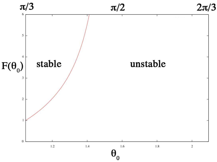
In order for rhombic lattice to be stable we require that . Thus, from Eq. ( 12) we have,
which reduces to,
or more simply
| (13) |
Using Eq. ( 2) we can write Eq. ( 13) as the condition for stability.
| (14) |
which can be rearranged to give
or,
which can be written as
| (15) |
plotting , see Fig (7), we find that depending on the ratio the rhombic lattice is either stable or unstable as a function of the rhombic angle .
Condition for stability for displacement along the direction
We now turn to the alternative case where the perturbation is along the direction and show that it is always unstable. In this case the condition for stability follows exactly as above except that the role of the indices and are interchanged, so that Eq. ( 14) becomes
| (16) |
Simplifying Eq. ( 14) gives the condition
Conclusion regarding stability
The combination of the two above conditions yields the result that a rhombic lattice is always unstable with respect to at least one of the distortions considered.
V Line-slip structures

As noted previously, for specific values of the periodicity vector it is possible to wrap a symmetric disk packing onto the surface of a cylinder. However, around these special points there exist variety of line-slip structures (see Fig (3c) which have packing fractions that vary continuously (and usually linearly) from the value of the symmetric arrangement. Here we will analyse these variations close to the symmetric structures.
Around each symmetric arrangement there are a total of six line slips, two for each of the primitive lattice vectors of the triangular lattice. Let us describe one of these line-slip arrangements with reference to the symmetric packing [5,4,1]. Fig (8) shows the symmetric arrangement , we allow the highlighted lattice row to slide in the direction. Ultimately this continues until the symmetric arrangement is reached. Note that in this case four lattice rows remain fixed while one is allowed to vary. Similarly instead the slip could have been in the direction (i.e. the opposite direction) which would have lead to the state . There are two other lattice directions and for each there are two possibilities (and in each case the number of rows which remain fixed depends on the direction of the line-slip). This gives the total of six.
We will analyse the variation of density with for line-slip structures close to the symmetric ones. We will derive the first and second order derivatives at these points which may be used in an expansion of the form,
| (17) |
This serves to elucidate many of the qualitative features of the numerical results, i.e. degeneracies and the choice of the line-slip which gives the maximum density.

We begin with the construction shown in Fig (9a). This shows an equilateral triangle whose sides can be traversed in a anti-clockwise direction by following the unit primitive vectors , and . Assume that the periodicity vector terminates on one of the vertices labelled , or .
For purposes of demonstration let us assume that the periodicity vector terminates on vertex . Then as shown in Fig (9b), can be perturbed by a rotation by an angle about axis centred on vertex (i.e. a rotation about tail of the vector ) . Let us denote the change in by the vector . This can be decomposed into a component parallel to and (perpendicular to this) is a component parallel to , we have
Alternatively if the rotation is centred on vertex (i.e. a rotation about the head of the vector ), as shown in Fig (9c), the change in is given by,
In general, for the th side of the triangle the variation in is
where distinguishes between perturbations due to a rotation about an axis at the head or the tail of the vector . Expanding to second order in gives,
Thus the length of the periodicity vector is given by
expanding in powers of yields
where the leading order term is
The coefficient of the linear term is found to be,
where denote the phyllotactic coefficients as described in section II. The function is defined as and .
Here, and in what follows, we use square brackets to indicate a modulo function so
such that and .
The coefficient of the second order term is
Similarly the average surface density of a triangular lattice is given by
which can be expanded in terms of , so that to second order we have
where
and
and
First order derivatives
Thus we have
| (18) |
The implications of Eq. ( 18) are as follows. If we confine attention to the linear variation of with around a symmetric structure, there are six possibilities for line-slip, as already stated, which fall into three degenerate pairs. In general two are in the “forward” direction, four in the “backward” direction, or vice versa. This pattern was evident in our earlier numerical work, but not understood. As for the magnitudes of the slopes, these are given by Eq. ( 18).
As an example we plot in Fig (10) the expansion given by Eq. ( 17) up to the linear term close to the symmetric packing [5,4,1] (see appendix A for the numerical values of the gradients). The expected the gradients are degenerate, so that although in general we expect six distinct line-slip structures there are only three distinct values for the gradients.

Second order derivatives
Clearly the gradient of the density of the various line-slip packings does not fully determine which line-slip packing has the highest density close to the maximal packing point. In order to distinguish between these proceed to the second derivative, which is evaluated as,
| (19) |
In Fig (11) we plot the expansion given Eq. ( 17) up to the second order term (again see appendix A for the numerical values) close to the symmetric packing [5,4,1]. Each line-slip packing is shown by a solid coloured curve and the corresponding approximation is give by a dashed line of the same colour.
Thus the expansion Eq. ( 17) can be used to interpolate between the symmetric close-packed structures. This procedure can reproduce very well the extensive results previously reported for the densities of the intermediate line-slip structures.

VI Conclusions
The problem of disk packing on a cylinder has turned out to be surprisingly rich in detail. In this paper we have shown that much of this can be accounted for analytically, offering definite rules for the densest structures.
We were originally led into this subject by a study of sphere packings in cylinders. The present results also help to shed some light on the corresponding sphere packings, at least qualitatively.
When we began the analysis it seemed only relevant to cylindrical packings of hard disks or spheres. That is the occurrence of the line-slip structures was seen as a feature to be associated with perfectly hard constituents. This is not quite correct. Systems comprised of softly interacting particles, such as those studied by Wood, et al [7], can exhibit this feature and we will pursue this in future work using the present results as a starting point.
VII Acknowledgements
AM acknowledges the support of the German Science Foundation (DFG) through the research group “Geometry and Physics of Spatial Random Systems” under grant no SCHR-1148/3-1. DW acknowledges the hospitality of Institut für Theoretische Physik I, Fried.-Alex.-Universität Erlangen-Nürnberg.
Appendix A
Taking for example the symmetric packing we evaluate the first and second derivatives (as described in section V). The table below gives the numerical values of the derivatives, accompanied by the appropriate indices as used in Eq. ( 18) and Eq. ( 19).
| 1 | 1 | 1 | 4 | 4 | 1 | 0.882 | 32.524 | |
| 1 | -1 | 1 | 4 | -5 | -1 | -0.706 | -4.465 | |
| 2 | 1 | 4 | -5 | -5 | -1 | -0.176 | 0.500 | |
| 2 | -1 | 4 | -5 | 1 | 1 | 0.881 | 4.234 | |
| 3 | 1 | -5 | 1 | 1 | 1 | -0.706 | 2.433 | |
| 3 | -1 | -5 | 1 | 4 | 1 | -0.176 | 0.479 |
References
- [1] A. Mughal, H.K. Chan, and D. Weaire, Physical Review Letters 106, 115704 (2011).
- [2] A. Mughal, D.W. H. K. Chan, and S. Hutzler, Physical Review E 85, 051305 (2012).
- [3] A. Mughal, Philosophical Magazine 93, 4070 (2011).
- [4] G.T. Pickett, M. Gross, and H. Okuyama, Physical Review Letters 85, 3652 (2000).
- [5] H. Chan, Philosophical Magazine 93, 4057 (2013).
- [6] H.K. Chan, Physical Review E 84, 050302 (2011).
- [7] D. Wood, C. Santangelo, and A. Dinsmore, Soft Matter 9, 10016 (2013).
- [8] N. Pittet, P. Boltenhagen, N. Rivier, and D. Weaire, Europhysics Letters 35, 547 (1996).
- [9] D. Weaire, S. Hutzler, and N. Pittet, Forma 7, 259 (1992).
- [10] P. Boltenhagen, N. Pittet, and N. Rivier, Europhysics Letters 43, 690 (1998).