Monte Carlo Non-Local Means: Random
Sampling for Large-Scale Image FilteringThanks: The authors are with the School of Engineering and Applied Sciences, Harvard University, Cambridge, MA 02138, USA. E-mails: {schan,zickler,yuelu}@seas.harvard.edu.Thanks: This work was supported in part by the Croucher Foundation Post-doctoral Research Fellowship (2012-2013), and in part by the U.S. National Science Foundation under Grant CCF-1319140. Preliminary material in this paper was presented at the 38th IEEE International Conference on Acoustics, Speech and Signal Processing (ICASSP), Vancouver, May 2013.Thanks: This paper follows the concept of reproducible research. All the results and examples presented in the paper are reproducible using the code and images available online at http://lu.seas.harvard.edu/.

In recent years, the image processing community has witnessed a wave of research aimed at developing new image denoising algorithms that exploit similarities between non-local patches in natural images. Most of these can be traced back to the non-local means (NLM) denoising algorithm of Buades et al. [1, 3] proposed in 2005. Although it is no longer the state-of-the-art method (see, e.g., [6, 4] for some more recent leading algorithms), NLM remains one of the most influential algorithms in the current denoising literature.

Given a noisy image, the NLM algorithm uses two sets of image patches for denoising. The first is a set of noisy patches $\mathcal{Y}=\{\boldsymbol{y}_{1},\ldots,\boldsymbol{y}_{m}\}$, where $\boldsymbol{y}_{i}\in\mathbb{R}^{d}$ is a $d$-dimensional (i.e., $d$-pixel) patch centered at the $i$th pixel of the noisy image. The second set, $\mathcal{X}=\{\boldsymbol{x}_{1},\ldots,\boldsymbol{x}_{n}\}$, contains patches that are obtained from some reference images. Conceptually, NLM simply replaces each $i$th noisy pixel with a weighted average of pixels in the reference set. Specifically, the filtered value at the $i$th pixel (for $1\leq i\leq m$) is given by

where $x_{j}$ denotes the value of the center pixel of the $j$th reference patch $\boldsymbol{x}_{j}\in\mathcal{X}$, and the weights $\left\{w_{i,j}\right\}$ measure the similarities between the patches $\boldsymbol{y}_{i}$ and $\boldsymbol{x}_{j}$. A standard choice for the weights is

where $h_{r}$ is a scalar parameter determined by the noise level, and $\lVert\cdot\rVert_{\boldsymbol{\Lambda}}$ is the weighted $\ell_{2}$-norm with a diagonal weight matrix $\boldsymbol{\Lambda}$, i.e., $\|\boldsymbol{y}_{i}-\boldsymbol{x}_{j}\|_{\boldsymbol{\Lambda}}^{2}\overset{\text{def}}{=}(\boldsymbol{y}_{i}-\boldsymbol{x}_{j})^{T}\boldsymbol{\Lambda}(\boldsymbol{y}_{i}-\boldsymbol{x}_{j})$.

In most implementations of NLM (see, e.g., [5, 6, 7, 8, 9, 10, 11]), the denoising process is based on a single image: the reference patches $\mathcal{X}$ are the same as the noisy patches $\mathcal{Y}$. We refer to this setting, when $\mathcal{X}=\mathcal{Y}$, as internal denoising. This is in contrast to the setting in which the set of reference patches $\mathcal{X}$ come from external image databases [12, 13, 14], which we refer to as external denoising. For example, $15,000$ images (corresponding to a reference set of $n\approx 10^{10}$ patches) were used in [13, 14]. One theoretical argument for using large-scale external denoising was provided in [13]: It is shown that, in the limit of large reference sets (i.e., when $n\rightarrow\infty$), external NLM converges to the minimum mean squared error estimator of the underlying clean images.

Despite its strong performance, NLM has a limitation of high computational complexity. It is easy to see that computing all the weights $\{w_{i,j}\}$ requires $\mathcal{O}(mnd)$ arithmetic operations, where $m,n,d$ are, respectively, the number of pixels in the noisy image, the number of reference patches used, and the patch dimension. Additionally, about $\mathcal{O}(mn)$ operations are needed to carry out the summations and multiplications in (1) for all pixels in the image. In the case of internal denoising, these numbers are nontrivial since current digital photographs can easily contain tens of millions of pixels (i.e., $m=n\sim 10^{7}$ or greater). For external denoising with large reference sets (e.g., $n\sim 10^{10}$), the complexity is even more of an issue, making it very challenging to fully utilize the vast number of images that are readily available online and potentially useful as external databases.

The high complexity of NLM is a well-known challenge. Previous methods to speed up NLM can be roughly classified in the following categories:

1. Reducing the reference set $\mathcal{X}$. If searching through a large set $\mathcal{X}$ is computationally intensive, one natural solution is to pre-select a subset of $\mathcal{X}$ and perform computation only on this subset [1, 16, 17]. For example, for internal denoising, a spatial weight $w^{s}_{i,j}$ is often included so that

A common choice of the spatial weight is

where $d_{i,j}$ and $d^{\prime}_{i,j}$ are, respectively, the Euclidean distance and the $\ell_{\infty}$ distance between the spatial locations of the $i$th and $j$th pixels; $\mathbb{I}$ is the indicator function; and $\rho$ is the width of the spatial search window. By tuning $h_{s}$ and $\rho$, one can adjust the size of $\mathcal{X}$ according to the heuristic that nearby patches are more likely to be similar.

2. Reducing dimension $d$. The patch dimension $d$ can be reduced by several methods. First, SVD projection [18, 19, 10, 20] can be used to project the $d$-dimensional patches onto a lower dimensional space spanned by the principal components computed from $\mathcal{X}$. Second, the integral image method [21, 22, 23] can be used to further speed up the computation of $\|\boldsymbol{y}_{i}-\boldsymbol{x}_{j}\|_{\boldsymbol{\Lambda}}^{2}$. Third, by assuming a Gaussian model on the patch data, a probabilistic early termination scheme [24] can be used to stop computing the squared patch difference before going through all the pixels in the patches.

3. Optimizing data structures. The third class of methods embed the patches in $\mathcal{X}$ and $\mathcal{Y}$ in some form of optimized data structures. Some examples include the fast bilateral grid [25], the fast Gaussian transform [26], the Gaussian KD tree [27, 4], the adaptive manifold method [5], and the edge patch dictionary [30]. The data structures used in these algorithms can significantly reduce the computational complexity of the NLM algorithm. However, building these data structures often requires a lengthy pre-processing stage, or require a large amount of memory, thereby placing limits on one’s ability to use large reference patch sets $\cal X$. For example, building a Gaussian KD tree requires the storage of $\mathcal{O}(nd)$ double precision numbers (see, e.g., [4, 31].)

In this paper, we propose a randomized algorithm to reduce the computational complexity of NLM for both internal and external denoising. We call the method Monte Carlo Non-Local Means (MCNLM), and the basic idea is illustrated in Figure 1 for the case of internal denoising. For each pixel $i$ in the noisy image, we randomly select a set of $k$ reference pixels according to some sampling pattern and compute a $k$-subset of the weights $\{w_{i,j}\}_{j=1}^{n}$ to form an approximated solution to (1). The computational complexity of MCNLM is $\mathcal{O}(mkd)$, which can be significantly lower than the original complexity $\mathcal{O}(mnd)$ when only $k\ll n$ weights are computed. Furthermore, since there is no need to re-organize the data, the memory requirement of MCNLM is $\mathcal{O}(m+n)$. Therefore, MCNLM is scalable to large reference patch sets $\mathcal{X}$, as we will demonstrate in Section V.

The two main contributions of this paper are as follows.

1. Performance guarantee. MCNLM is a randomized algorithm. It would not be a useful one if its random outcomes fluctuated widely in different executions on the same input data. In Section III, we address this concern by showing that, as the size of the reference set $\mathcal{X}$ increases, the randomized MCNLM solutions become tightly concentrated around the original NLM solution. In particular, we show in Theorem 1 (and Proposition 1) that, for any given sampling pattern, the probability of having a large deviation from the original NLM solution drops exponentially as the size of $\mathcal{X}$ grows.

2. Optimal sampling patterns. We derive optimal sampling patterns to minimize the approximation error probabilities established in our performance analysis. We show that seeking the optimal sampling pattern is equivalent to solving a variant of the classical water-filling problem, for which a closed-form expression can be found (see Theorem 2). We also present two practical sampling pattern designs that exploit partial knowledge of the pairwise similarity weights.

The rest of the paper is organized as follows. After presenting the MCNLM algorithm and discuss its basic properties in Section II, we analyze the performance in Section III and derive the optimal sampling patterns in Section IV. Experimental results are given in Section V, and concluding remarks are given in Section VI.

As discussed in Section I, computing all the weights $\{w_{i,j}\}_{1\leq i\leq m,1\leq j\leq n}$ is computationally prohibitive when $m$ and $n$ are large. To reduce the complexity, the basic idea of MCNLM is to randomly select a subset of $k$ representatives of $\{w_{i,j}\}$ (referred to as samples) to approximate the sums in the numerator and denominator in (1). The sampling process in the proposed algorithm is applied to each of the $m$ pixels in the noisy image independently. Since the sampling step and subsequent computations have the same form for each pixel, we shall drop the pixel index $i$ in $\left\{w_{i,j}\right\}$, writing the weights as $\left\{w_{j}\right\}_{1\leq j\leq n}$ for notational simplicity.

The sampling process of MCNLM is determined by a sequence of independent random variables $\{I_{j}\}_{j=1}^{n}$ that take the value $0$ or $1$ with the following probabilities

The $j$th weight $w_{j}$ is sampled if and only if $I_{j}=1$. In what follows, we assume that $0<p_{j}\leq 1$, and refer to the vector of all these probabilities $\boldsymbol{p}\mathop{\overset{\mbox{\tiny{def}}}{=}}[p_{1},\ldots,p_{n}]^{T}$ as the sampling pattern of the algorithm.

The ratio between the number of samples taken and the number of reference patches in $\mathcal{X}$ is a random variable

of which the expected value is

We refer to $S_{n}$ and $\xi$ as the empirical sampling ratio and the average sampling ratio, respectively. $\xi$ is an important parameter of the MCNLM algorithm. The original (or “full”) NLM corresponds to the setting when $\xi=1$: In this case, $\boldsymbol{p}=\boldsymbol{1}\overset{\text{def}}{=}[1,\ldots,1]^{T}$, so that all the samples are selected with probability one.

Given a set of random samples from $\mathcal{X}$, we approximate the numerator and denominator in (1) by two random variables

where the argument $\boldsymbol{p}$ emphasizes the fact that the distributions of $A$ and $B$ are determined by the sampling pattern $\boldsymbol{p}$.

It is easy to compute the expected values of $A(\boldsymbol{p})$ and $B(\boldsymbol{p})$ as

Thus, up to a common multiplicative constant $1/n$, the two random variables $A(\boldsymbol{p})$ and $B(\boldsymbol{p})$ are unbiased estimates of the true numerator and denominator, respectively.

The full NLM result $z$ in (1) is then approximated by

In general, $\mathbb{E}[Z(\boldsymbol{p})]=\mathbb{E}\left[\frac{A(\boldsymbol{p})}{B(\boldsymbol{p})}\right]\neq\frac{\mathbb{E}[A(\boldsymbol{p})]}{\mathbb{E}[B(\boldsymbol{p})]}=z$, and thus $Z(\boldsymbol{p})$ is a biased estimate of $z$. However, we will show in Section III that the probability of having a large deviation in $|Z(\boldsymbol{p})-z|$ drops exponentially as $n\rightarrow\infty$. Thus, for a large $n$, the MCNLM solution (11) can still form a very accurate approximation of the original NLM solution (1).

Algorithm 1 shows the pseudo-code of MCNLM for internal denoising. We note that, except for the Bernoulli sampling process, all other steps are identical to the original NLM. Therefore, MCNLM can be thought of as adding a complementary sampling process on top of the original NLM. The marginal cost of implementation is thus minimal.

The mathematical tool we use to analyze the proposed MCNLM algorithm comes from the probabilistic large deviations theory [32]. This theory has been widely used to quantify the following phenomenon: A smooth function $f(X_{1},\ldots,X_{n})$ of a large number of independent random variables $X_{1},\ldots,X_{n}$ tends to concentrate very tightly around its mean $\mathbb{E}[f(X_{1},\ldots,X_{n})]$. Roughly speaking, this concentration phenomenon happens because, while $X_{1},\ldots,X_{n}$ are individually random in nature, it is unlikely for many of them to work collaboratively to alter the overall system by a significant amount. Thus, for large $n$, the randomness of these variables tends to be “canceled out” and the function $f(X_{1},\ldots,X_{n})$ stays roughly constant.

To gain insights from a concrete example, we first apply the large deviations theory to study the empirical sampling ratio $S_{n}$ as defined in (6). Here, the independent random variables are the Bernoulli random variables $\left\{I_{j}\right\}_{1\leq j\leq n}$ introduced in (5), and the smooth function $f(\cdot)$ computes their average.

It is well known from the law of large numbers (LLN) that the empirical mean $S_{n}$ of a large number of independent random variables stays very close to the true mean, which is equal to the average sampling ratio $\xi$ in our case. In particular, by the standard Chebyshev inequality [33], we know that

for every positive $\varepsilon$.

One drawback of the bound in (12) is that it is overly loose, providing only a linear rate of decay for the error probabilities as $n\rightarrow\infty$. In contrast, the large deviations theory provides many powerful probability inequalities which often lead to much tighter bounds with exponential decays. In this work, we will use one particular inequality in the large deviations theory, due to S. Bernstein [34]:

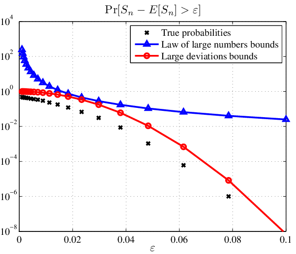
To see how Bernstein’s inequality can give us a better probability bound for the empirical sampling ratio $S_{n}$, we note that $X_{j}=I_{j}$ in our case. Thus, $M=1$ and $\mathbb{E}[S_{n}]=\xi$. Moreover, if the sampling pattern is uniform, i.e., $\boldsymbol{p}=[\xi,\ldots,\xi]^{T}$, we have $\frac{1}{n}\sum_{j=1}^{n}\mathrm{Var}[X_{j}]=\frac{1}{n}\sum_{j=1}^{n}p_{j}(1-p_{j})=\xi(1-\xi)$. Substituting these numbers into (13) yields an exponential upper bound on the error probability, which is plotted and compared in Figure 4 against the LLN bound in (12) and against the true probabilities estimated by Monte Carlo simulations. It is clear that the exponential bound provided by Bernstein’s inequality is much tighter than that provided by LLN.

We now derive a general bound for the error probabilities of MCNLM. Specifically, for any $\varepsilon>0$ and any sampling pattern $\boldsymbol{p}$ satisfying the conditions that $0<p_{j}\leq 1$ and $\frac{1}{n}\sum_{j=1}^{n}p_{j}=\xi$, we want to study

where $z$ is the full NLM result defined in (1) and $Z(\boldsymbol{p})$ is the MCNLM estimate defined in (11).

Since the error probability bound in (15) holds for all sampling patterns $\boldsymbol{p}$, we will use (15) to design optimal nonuniform sampling patterns in Section IV. But before we discuss that, we first consider the special case where $\boldsymbol{p}$ is a uniform sampling pattern to provide a convenient and easily interpretable bound on the error probabilities.

To interpret (16), we note that, for large $n$, the first term on the right-hand side of (16) is negligible. For example, when $n=10^{4}$ and $\xi=0.01$, we have $e^{-n\xi}=3.7\times 10^{-44}$. Thus, the error probability bound is dominated by the second term, whose negative exponent is determined by four factors:

1. The size of the reference set $\mathcal{X}$. If all other parameters are kept fixed or strictly bounded below by some positive constants, the error probability goes to zero as an exponential function of $n$. This shows that the random estimates obtained by MCNLM can be very accurate, when the size of the image (for internal denoising) or the size of the dictionary (for external denoising) is large.

2. Sampling ratio $\xi$. To reduce the sampling ratio $\xi$ while still keeping the error probability small, a larger $n$, inversely proportional to $\xi$, is needed.

3. Precision $\varepsilon$. Note that the function $f(\varepsilon)$ in (16) is of order $\mathcal{O}(\varepsilon^{2})$ for small $\varepsilon$. Thus, with all other terms fixed, a $k$-fold reduction in $\varepsilon$ requires a $k^{2}$-fold increase in $n$ or $\xi$.

4. Patch redundancy $\mu_{B}$. Recall that $\mu_{B}=\frac{1}{n}\sum_{j=1}^{n}w_{j}$, with the weights $\left\{w_{j}\right\}$ measuring the similarities between a noisy patch $\boldsymbol{y}_{i}$ and all patches $\{\boldsymbol{x}_{j}\}_{j=1}^{n}$ in the reference set $\mathcal{X}$. Thus, $\mu_{B}$ serves as an indirect measure of the number of patches in $\mathcal{X}$ that are similar to $\boldsymbol{y}_{i}$. If $\boldsymbol{y}_{i}$ can find many similar (redundant) patches in $\mathcal{X}$, its corresponding $\mu_{B}$ will be large and so a relatively small $n$ will be sufficient to make the probability small; and vice versa.

Using the simplified expression in (16), we derive in Appendix A-C the following upper bound on the mean squared error (MSE) of the MCNLM estimation:

The starting point of seeking an optimal sampling pattern is the general probability bound provided by Theorem 1. A challenge in applying this probability bound in practice is that the right-hand side of (15) involves the complete set of weights $\left\{w_{j}\right\}$ and the full NLM result $z$. One can of course compute these values, but doing so will defeat the purpose of random sampling, which is to speed up NLM by not computing all the weights $\left\{w_{j}\right\}$. To address this problem, we assume that

where the upper bounds $\left\{b_{j}\right\}$ are either known a priori or can be efficiently computed. We will provide concrete examples of such upper bounds in Section IV-B. For now, we assume that the bounds $\left\{b_{j}\right\}$ have already been obtained.

Using (20) and noting that $0\leq x_{j},z\leq 1$ (and thus $|x_{j}-z|\leq 1$), we can see that the parameters $\left\{\alpha_{j},\beta_{j}\right\}$ in (15) are bounded by

respectively. It then follows from (15) that

where $M\overset{\text{def}}{=}\left(\mu_{B}\varepsilon\right)/(6(1+\varepsilon))$.

Given the average sampling ratio $\xi$, we seek sampling patterns $\boldsymbol{p}$ to minimize the probability bound in (21), so that the random MCNLM estimate $Z(\boldsymbol{p})$ will be tightly concentrated around the full NLM result $z$. Equivalently, we solve the following optimization problem.

The optimization formulated has a closed-form solution stated as below. The derivation is given in Appendix A-D.

To construct the optimal sampling pattern prescribed by Theorem 2, we need to find $\left\{b_{j}\right\}$, which are the upper bounds on the true similarity weights $\left\{w_{j}\right\}$. At one extreme, the tightest upper bounds are $b_{j}=w_{j}$, but this oracle scheme is not realistic as it requires that we know all the weights $\left\{w_{j}\right\}$. At the other extreme, we can use the trivial upper bound $b_{j}=1$. It is easy to verify that, under this setting, the sampling pattern in (40) becomes the uniform pattern, i.e., $p_{j}=\xi$ for all $j$. In what follows, we present two choices for the upper bounds that can be efficiently computed and that can utilize partial knowledge of $w_{j}$.

A benchmark of ten standard test images are used for this experiment. For each image, we add zero-mean Gaussian noise with standard deviations equal to $\sigma=\frac{10}{255},\frac{20}{255},\frac{30}{255},\frac{40}{255},\frac{50}{255}$ to simulate noisy images at different PSNR levels. Two choices of the spatial search window size are used: $21\times 21$ and $35\times 35$, following the original configurations used in [1].

The parameters of MCNLM are as follows: The patch size is $5\times 5$ (i.e., $d=25$) and $\boldsymbol{\Lambda}=\boldsymbol{I}/d$. For each choice of the spatial search window size (i.e., $\rho=21$ or $\rho=35$), we define $h_{s}=(\lfloor\rho/2\rfloor)/3$ so that three standard deviations of the spatial Gaussian will be inside the spatial search window. The intensity parameter is set to $h_{r}=1.3\sigma/255$.

In this experiment, we use the spatial information bound (26) to compute the optimal sampling pattern in (40). Incorporating additional intensity information as in (27) would further improve the performance, but we choose not to do so because the PSNR gains are found to be moderate in this case due to the relatively small size of the spatial search window. Five average sampling ratios, $\xi=0.05,0.1,0.2,0.5,1$, are evaluated. We note that when $\xi=1$, MCNLM is identical to the full NLM.

For comparisons, we test the Gaussian KD tree (GKD) algorithm [4] with a C++ implementation (ImageStack [40]) and the adaptive manifold (AM) algorithm [5] with a MATLAB implementation provided by the authors. To create a meaningful common ground for comparison, we adapt MCNLM as follows: First, since both GKD and AM use SVD projection [20] to reduce the dimensionality of patches, we also use in MCNLM the same SVD projection method by computing the 10 leading singular values. The implementation of this SVD step is performed using an off-the-shelf MATLAB code [41]. We also tune the major parameters of GKD and AM for their best performance, e.g., for GKD we set $h_{r}=1.3\sigma/255$ and for AM we set $h_{r}=2\sigma/255$. Other parameters are kept at their default values as reported in [4], [5]. For completeness, we also show the results of BM3D [6].

Table I and Table II summarize the results of the experiment. Additional results, with visual comparison of denoised images, can be found in the supplementary technical report [39]. Since MCNLM is a randomized algorithm, we report the average PSNR values of MCNLM over 24 independent runs using random sampling pattern and 20 independent noise realizations. The standard deviations of the PSNR values over the 24 random sampling patterns are shown in Table II. The results show that for the 10 images, even at a very low sampling ratio, e.g., $\xi=0.1$, the averaged performance of MCNLM (over 10 testing images) is only about $0.35$ dB to $0.7$ dB away (depending on $\sigma$) from the full NLM solution. When the sampling ratio is further increased to $\xi=0.2$, the PSNR values become very close (about a $0.09$ dB to $0.2$ dB drop depending on $\sigma$) to those of the full solution.

In Table III we report the runtime of MCNLM, GKD and AM. Since the three algorithms are implemented in different environments, namely, MCNLM in MATLAB/C++ (.mex), GKD in C++ with optimized library and data-structures, and AM in MATLAB (.m), we caution that Table III is only meant to provide some rough references on computational times. For MCNLM, its speed improvement over the full NLM can be reliably estimated by the average sampling ratio $\xi$.

We note that the classical NLM algorithm is no longer the state-of-the-art in image denoising. It has been outperformed by several more recent approaches, e.g., BM3D [6] (See Table I and II) and global image denoising [4]. Thus, for internal (i.e., single-image) denoising, the contribution of MCNLM is mainly of a theoretical nature: It provides the theoretical foundation and a proof-of-concept demonstration to show the effectiveness of a simple random sampling scheme to accelerate the NLM algorithm. More work is needed to explore the application of similar ideas to more advanced image denoising algorithms.

As we will show in the following, the practical usefulness of the proposed MCNLM algorithm is more significant in the setting of external dictionary-based denoising, for which the classical NLM is still a leading algorithm enjoying theoretical optimality as the dictionary size grows to infinity [13].

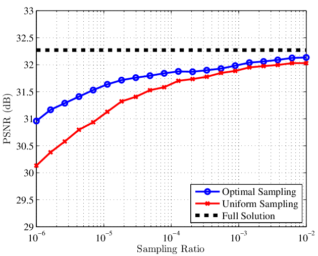
To test MCNLM for external dictionary-based image denoising, we consider the dataset of Levin and Nadler [13], which contains about 15,000 training images (about $n\approx 10^{10}$ image patches) from the LabelMe dataset [42]. For testing, we use a separate set of 2000 noisy patches, which are mutually exclusive from the training images. The results are shown in Figure 8.

References

- [1] A. Buades, B. Coll, and J. Morel, “A review of image denoising algorithms, with a new one,” Multiscale Model. Simul., vol. 4, no. 2, pp. 490–530, 2005.
- [2] A. Buades, B. Coll, and J. Morel, “Denoising image sequences does not require motion estimation,” in Proc. IEEE Conf. Advanced Video and Signal Based Surveillance (AVSS), Sep. 2005, pp. 70–74.
- [3] K. Dabov, A. Foi, V. Katkovnik, and K. Egiazarian, “Image denoising by sparse 3D transform-domain collaborative filtering,” IEEE Trans. Image Process., vol. 16, no. 8, pp. 2080–2095, Aug. 2007.
- [4] H. Talebi and P. Milanfar, “Global image denoising,” IEEE Trans. Image Process., vol. 23, no. 2, pp. 755–768, Feb. 2014.
- [5] M. Protter, M. Elad, H. Takeda, and P. Milanfar, “Generalizing the non-local-means to super-resolution reconstruction,” IEEE Trans. Image Process., vol. 18, no. 1, pp. 36–51, Jan. 2009.
- [6] J. Mairal, F. Bach, J. Ponce, G. Sapiro, and A. Zisserman, “Non-local sparse models for image restoration,” in Proc. IEEE Int. Conf. Computer Vision (ICCV), Oct. 2009, pp. 2272–2279.
- [7] K. Chaudhury and A. Singer, “Non-local patch regression: Robust image denoising in patch space,” in Proc. IEEE Int. Conf. Acoustics, Speech and Signal Process. (ICASSP), 2013, available online at http://arxiv.org/abs/1211.4264.
- [8] P. Milanfar, “A tour of modern image filtering,” IEEE Signal Processing Magazine, vol. 30, pp. 106–128, Jan. 2013.
- [9] W. Dong, L. Zhang, G. Shi, and X. Li, “Nonlocally centralized sparse representation for image restoration,” IEEE Trans. Image Process., vol. 22, no. 4, pp. 1620–1630, Apr. 2013.
- [10] D. Van De Ville and M. Kocher, “SURE-based non-local means,” IEEE Signal Process. Lett., vol. 16, no. 11, pp. 973–976, Nov. 2009.
- [11] C. Kervrann and J. Boulanger, “Optimal spatial adaptation for patch-based image denoising,” IEEE Trans. Image Process., vol. 15, no. 10, pp. 2866–2878, Oct. 2006.
- [12] M. Zontak and M. Irani, “Internal statistics of a single natural image,” in Proc. IEEE Conf. Computer Vision and Pattern Recognition (CVPR), Jun. 2011, pp. 977–984.
- [13] A. Levin and B. Nadler, “Natural image denoising: Optimality and inherent bounds,” in Proc. IEEE Conf. Computer Vision and Pattern Recognition (CVPR), Jun. 2011, pp. 2833–2840.
- [14] A. Levin, B. Nadler, F. Durand, and W. Freeman, “Patch complexity, finite pixel correlations and optimal denoising,” in Proc. 12th European Conf. Computer Vision (ECCV), Oct. 2012, vol. 7576, pp. 73–86.
- [15] M. Mahmoudi and G. Sapiro, “Fast image and video denoising via nonlocal means of similar neighborhoods,” IEEE Signal Process. Lett., vol. 12, no. 12, pp. 839–842, Dec. 2005.
- [16] P. Coupe, P. Yger, and C. Barillot, “Fast non local means denoising for 3D MR images,” in Proc. Medical Image Computing and Computer-Assisted Intervention (MICCAI), 2006, pp. 33–40.
- [17] T. Brox, O. Kleinschmidt, and D. Cremers, “Efficient nonlocal means for denoising of textural patterns,” IEEE Trans. Image Process., vol. 17, no. 7, pp. 1083–1092, Jul. 2008.
- [18] T. Tasdizen, “Principal components for non-local means image denoising,” in Proc. IEEE Int. Conf. Image Process. (ICIP), Oct. 2008, pp. 1728 –1731.
- [19] J. Orchard, M. Ebrahimi, and A. Wong, “Efficient nonlocal-means denoising using the SVD,” in Proc. IEEE Int. Confe. Image Process. (ICIP), Oct. 2008, pp. 1732 –1735.
- [20] D. Van De Ville and M. Kocher, “Nonlocal means with dimensionality reduction and SURE-based parameter selection,” IEEE Trans. Image Process., vol. 20, no. 9, pp. 2683 –2690, Sep. 2011.
- [21] J. Darbon, A. Cunha, T. Chan, S. Osher, and G. Jensen, “Fast nonlocal filtering applied to electron cryomicroscopy,” in Proc. IEEE Int. Sym. Biomedical Imaging, 2008, pp. 1331–1334.
- [22] J. Wang, Y. Guo, Y. Ying, Y. Liu, and Q. Peng, “Fast non-local algorithm for image denoising,” in Proc. IEEE Int.Conf. Image Process. (ICIP), Oct. 2006, pp. 1429–1432.
- [23] V. Karnati, M. Uliyar, and S. Dey, “Fast non-local algorithm for image denoising,” in Proc. IEEE Int. Conf. Image Process. (ICIP), 2009, pp. 3873–3876.
- [24] R. Vignesh, B. Oh, and J. Kuo, “Fast non-local means (NLM) computation with probabilistic early termination,” IEEE Signal Process. Lett., vol. 17, no. 3, pp. 277–280, Mar. 2010.
- [25] S. Paris and F. Durand, “A fast approximation of the bilateral filter using a signal processing approach,” Int. J. Computer Vision, vol. 81, no. 1, pp. 24–52, Jan. 2009.
- [26] C. Yang, R. Duraiswami, N. Gumerov, and L. Davis, “Improved fast Gauss transform and efficient kernel density estimation,” in Proc. Int. Conf. Computer Vision (ICCV), Oct. 2003, pp. 664–671.
- [27] A. Adams, J. Baek, and M. A. Davis, “Fast high-dimensional filtering using the permutohedral lattice,” in Proc. EUROGRAPHICS, 2010, vol. 29, pp. 753–762.
- [28] A. Adams, N. Gelfand, J. Dolson, and M. Levoy, “Gaussian KD-trees for fast high-dimensional filtering,” in Proc. of ACM SIGGRAPH, 2009, Article No. 21.
- [29] E. Gastal and M. Oliveira, “Adaptive manifolds for real-time high-dimensional filtering,” ACM Trans. Graphics, vol. 31, no. 4, pp. 33:1–33:13, 2012.
- [30] H. Bhujle and S. Chaudhuri, “Novel speed-up strategies for non-local means denoising with patch and edge patch based dictionaries,” IEEE Trans. Image Process., vol. 23, no. 1, pp. 356–365, Jan. 2014.
- [31] S. Arietta and J. Lawrence, “Building and using a database of one trillion natural-image patches,” IEEE Computer Graphics and Applications, vol. 31, no. 1, pp. 9–19, Jan. 2011.
- [32] A. Dembo and O. Zeitouni, Large deviations techniques and applications, Springer, Berlin, 2010.
- [33] G. R. Grimmett and D. R. Stirzaker, Probability and Random Processes, Oxford University Press, 3rd edition, 2001.
- [34] S. Bernstein, The Theory of Probabilities, Gastehizdat Publishing House, Moscow, 1946.
- [35] S. H. Chan, T. Zickler, and Y. M. Lu, “Fast non-local filtering by random sampling: It works, especially for large images,” in Proc. IEEE Int. Conf. Acoust., Speech, Signal Process. (ICASSP), 2013, pp. 1603–1607.
- [36] R. Serfling, “Probability inequalities for the sum in sampling without replacement,” The Annals of Statistics, vol. 2, pp. 39–48, 1974.
- [37] F. Chung and L. Lu, “Concentration inequalities and martingale inequalities: a survey,” Internet Mathematics, vol. 3, no. 1, pp. 79–127, 2006.
- [38] P. Drineas, R. Kannan, and M. Mahoney, “Fast Monte Carlo algorithms for matrices I: Approximating matrix multiplication,” SIAM J. Computing, vol. 36, pp. 132–157, 2006.
- [39] S. H. Chan, T. Zickler, and Y. M. Lu, “Monte-Carlo non-local means: Random sampling for large-scale image filtering — Supplementary material,” Tech. Rep., Harvard University, 2013, [Online] http://arxiv.org/abs/1312.7366.
- [40] A. Adams, “Imagestack,” https://code.google.com/p/imagestack/.
- [41] G. Peyre, “Non-local means MATLAB toolbox,” http://www.mathworks.com/matlabcentral/fileexchange/13619.
- [42] B. Russell, A. Torralba, K. Murphy, and W. Freeman, “LabelMe: a database and web-based tool for image annotation,” Int. J. Computer Vision, vol. 77, no. 1-3, pp. 157–173, May 2008.
- [43] W. Feller, An Introduction to Probability Theory and its Applications, vol. 2, John Wiley & Sons, 2nd edition, 1971.
- [1] M. Mahmoudi and G. Sapiro, “Fast image and video denoising via nonlocal means of similar neighborhoods,” IEEE Signal Process. Lett., vol. 12, no. 12, pp. 839–842, Dec. 2005.
- [2] K. Murphy, Machine Learning: A Probabilistic Perspective, MIT Press, 2012.
- [3] A. Buades, B. Coll, and J. Morel, “Denoising image sequences does not require motion estimation,” in Proc. IEEE Conf. Advanced Video and Signal Based Surveillance (AVSS), Sep. 2005, pp. 70–74.
- [4] A. Adams, N. Gelfand, J. Dolson, and M. Levoy, “Gaussian KD-trees for fast high-dimensional filtering,” in Proc. of ACM SIGGRAPH, 2009, Article No. 21.
- [5] E. Gastal and M. Oliveira, “Adaptive manifolds for real-time high-dimensional filtering,” ACM Trans. Graphics, vol. 31, no. 4, pp. 33:1–33:13, 2012.
- [6] K. Dabov, A. Foi, V. Katkovnik, and K. Egiazarian, “Image denoising by sparse 3D transform-domain collaborative filtering,” IEEE Trans. Image Process., vol. 16, no. 8, pp. 2080–2095, Aug. 2007.