Fitting the Continuum Component of
A Composite SDSS Quasar Spectrum Using CMA-ESNote: Last revised August 24, 2026
Abstract
Fitting the continuum component of a quasar spectrum in UV/optical band is challenging due to contamination of numerous emission lines. Traditional fitting algorithms such as the least-square fitting and the Levenberg-Marquardt algorithm (LMA) are fast but are sensitive to initial values of fitting parameters. They cannot guarantee to find global optimum solutions when the object functions have multiple minima. In this work, we attempt to fit a typical quasar spectrum using the Covariance Matrix Adaptation Evolution Strategy (CMA-ES). The spectrum is generated by composing a number of real quasar spectra from the Sloan Digital Sky Survey (SDSS) quasar catalog data release 3 (DR3) so it has a higher signal-to-noise ratio. The CMA-ES algorithm is an evolutionary algorithm that is designed to find the global rather than the local minima. The algorithm we implemented achieves an improved fitting result than the LMA and unlike the LMA, it is independent of initial parameter values. We are looking forward to implementing this algorithm to real quasar spectra in UV/optical band.
Keywords:
methods: data analysis — methods: numerical — quasars: generalI Introduction
We have constructed a set of 161 composite quasar spectra binned in redshift and luminosity space from typical SDSS quasars. Spectra in the same bin are normalized and averaged, so each composite spectrum represents the average properties of the spectra in each bin. This is the first time this technique has been used to study the evolution over a wide range of luminosity () and redshift ().
We have tried two types of algorithms to derive a set of measurements from the composite spectra.
- •
The Levenberg-Marquardt algorithm (LMA) is designed to solve the multivariate least-squares curve fitting problem [10]. It interpolates between the Gauss-Newton algorithm (GNA) [5] and the method of gradient descent [2], but it is more robust than the GNA, which means that in many cases, LMA finds a solution even if it starts far from the final minimum. The fitting results using this algorithm are displayed in Fig. 1. This method has some limitations
- –
We found that to solve a problem with more than 10 free parameters, this algorithm is sensitive to initial values of parameters. We must provided an initial guess of the power-law (PL) component, and this estimate must be as close to the optimal value as possible.
- –
This algorithm does not work well for the iron templates, which do not have analytical expressions. The iron emission and the small blue bump (SBB) cannot be fit well simultaneously (see the over-production of model flux around 3700 Å). In addition, we could not use this method to find the proper velocity dispersions of the iron template because the available dispersion values are discrete.
- –
- •
Genetic algorithm (GA). GA is a search heuristic that mimics the process of natural evolution [3]. This heuristic is routinely used to generate useful solutions to optimization and search problems. A typical GA algorithm consists of initialization, selection, reproduction and termination. The solutions asymptotically converge to an optimal value under a given criteria. Vanden Berk wrote a program (not published) using this algorithm to fit the SDSS quasar spectra using GA, but this program has two disadvantages
- –
Instead of using the iron emission templates, each low ionization iron emission line is simulated using one or multiple Gaussian profiles. This requires over a hundred free parameters, which significantly slows down the fitting process. GA requires 5 – 10 minutes (using a typical desktop computer with a 2.0 GHz processor) to fit a composite quasar spectrum.
- –
Although the program can produce a nearly perfect fit, the result is unstable. There are a number of parameter combinations that can produce equally good fits and it is difficult to determine which is the physical solution.
- –
The limitations and disadvantages of these two methods motivate us to develop an evolutionary algorithm to fit the quasar spectrum. The CMA-ES is an evolutionary algorithm for difficult non-linear non-convex optimization problems in a continuous domain [8]. It is a second order approach to estimate a positive definite matrix within an iterative procedure (the covariance matrix). This approach makes the method feasible on non-separable and/or ill conditioned problems. Because this method does not require gradients, it is feasible on non-smooth and even non-continuous problems, as well as “noisy” problems. Previous results using LMA imply that the space of the objective function is not smooth as the solution varies depending on the initial guess [9]. The CMA-ES approach can overcome this problem.
The paper is outlined in the following way. In Section II, we describe the problem in detail; in Section III, we present the solution strategy in terms of each step applied in CMA-ES; in Section IV, we briefly describe some important issues that arose when developing the program; in Section V, we present our optimization results; and finally in Section VI, we discuss the limitations of our approach and potential extension of this work.
II Problem Description
We are aiming at fitting the underlying continuum of a composite quasar spectrum at , and (see Fig. 1). This continuum is fit by four components
- 1.
A power-law (PL) continuum, which takes the form . This component has two free parameters: the spectral index and the scaling factor . In principle, the variables do not have any constraints but previous studies have found that and 6–7.
- 2.
A small blue bump (SBB), which takes the form
(1) This component has three free parameters: Balmer temperature , Balmer optical depth , and scale factor . The scale factor should be positive; the other two parameters do not have constraints. Empirically, , and . Both and are in units of Å and Å.
- 3.
UV iron emission forest. This is a blend of many low ionization iron emission lines ranging from Å to 3090 Å. This component has three free parameters, the scale factor , velocity dispersion and relative shift 11 1 This is the shift of the template with respect to the quasar spectrum itself, not the redshift of the quasar relative to the observer.. The scale factor should be positive. The velocity dispersion can only be one of km s-1 (set by a template grid). In principle, can be any value but typically .
- 4.
Optical iron emission forest. This is a blend of many low ionization iron emission lines ranging from Å to Å. Similar to the UV template, this component also has three free parameters, the scale factor , velocity dispersion and relative shift . Again, can only be one of km s-1, and .
A summary of the free parameters and their permitted values are listed in Table 1. We use the reduced value as the objective function:
in which is the number of benchmark wavelength points, which is used to compare the model and the observed fluxes; is the number of variables; is the interpolated observed flux value at wavelength point ; is the expected (calculated) flux value at wavelength point , and is the interpolated observational uncertainty at wavelength point . In this problem, we have benchmark points and variables.
III Solution Strategy
We apply the CMA-ES as the method to solve this problem. This algorithm involves sampling, selection, cumulation and updating operations [6]. The problem is initialized as Table 2 and each parameter shown below such as , and are also described in Table 2. Each generation loop of consists the following steps.
- 1.
Generate and evaluate offspring
Vector has elements, and is an matrix (the covariant matrix). In this step, we apply a death penalty to the two velocity dispersion values and . If they fail to fall into the range of , we simply discard this value and re-draw a new set of random numbers. However, if the number of failures is greater than 10, we stop drawing and adopt the boundary value. When evaluating the fitness function, we apply a penalty term to the fitness function based on the value of redshift and , so that
The are the constrained items :
In the equations above, and, is the generation number.
- 2.
Sort offspring by the penalized function and compute the weighted mean. Although we sort the offspring using the penalized function, we still output the unpenalized function , because it reflects the real goodness-of-fit regardless of penalty term. In addition, involves the generation number , so even if the best decreases in the first few generations, it will increase after a certain point. After sorting the offspring ascendingly, we select the first offspring as the parents to calculate the weighted mean. The weighted mean after selecting offspring is
Note that is a matrix of and is selected from based on the fitness function so contains the best offspring and thus has the heaviest weight (see appendix).
- 3.
Cumulation: update the evolution paths. Conceptually, the evolution path is the path the strategy takes over a number of generation steps, which can be expressed as a sum of consecutive steps of the (weighted) mean . To accomplish this task, we iterate two path vectors, and , which represent the path of and the covariance matrix . Both and have two terms. The first term is the vector itself in the last iteration multiplied by a decay factor. This term causes the vector norm to decrease. The second term is based on the weighted mean of the selected offspring with a normalization factor and directs the evolution path to the optimal value. This step is a preparation to the covariance matrix adaption and step size adaption in the succeeding steps. The equations used to calculate these paths and the updates of evolution paths and , are shown below.
in which represents the array element in the inverse square root of matrix .
- 4.
Adapt covariance matrix . This is the essential part of the algorithm and the reason why it is named as the covariance-matrix adaption evolutionary algorithm. The adaption equation includes three terms. The first term is the covariance matrix itself multiplied by a decay factor. Again, this term decreases the norm of the covariance matrix. The second term is the rank one update plus a minor correction based on the evolutionary path ; This term can learn straight ridges in rather than function evaluations. The third term is the rank update which is based on the weighted cross product of the selected offspring. The rank update increases the possible learning rate in large populations and also reduces the number of necessary generations roughly from to [7]. Therefore, the rank update is the primary mechanism whenever a large population size is used (say ). The equation for adaption of covariance matrix is
in which , , and is an array of which each column is . Note that represents the selected and sorted offspring.
- 5.
Finally, we update the step size . The reason for a step control is that the covariance matrix update can hardly increase the variance in all directions simultaneously. In other words, the overall scale of search, the global step-size cannot be increased effectively [1]. In our investigation, we apply the path length control (cumulative step-size adaption) as recommended by [4]. The equation for adaption of step size is
- 6.
Correct . To ensure that is a symmetric matrix, we enforce symmetry by replacing the lower triangle elements with the upper triangle elements.
- 7.
We apply four criteria to terminate the generation loop
- (a)
The best fitness is below the pre-defined value.
- (b)
The number of generations is greater than the maximum number of generations allowed ().
- (c)
The change of the best fitness value is smaller than 0.05 for 20 consecutive generations.
- (d)
The change of the best fitness value is positive for 20 consecutive generations. Theoretically, this could never happen, but in practice it does when the objective function approaches the optimal value.
- (a)
IV Program Design
The coding design basically follows the flow of the loop in Section III; here we briefly mention some special aspects that arose when developing the code.
- •
To avoid reading the iron emission templates from hard drive each time we evaluate the fitness function, we upload template spectra of all the velocity dispersions before the generation loop. This requires a few seconds of some overhead computational time, but it significantly reduces the computational time required to evaluate the objective function. In each generation, we must evaluate the objective function at least 220 times (in the default situation).
- •
The available values of and are not continuous. As a result, we must perform a discretization to make sure that they are integer multiples of 500 km s-1 before evaluating the fitness function.
- •
To compute , we first must find the eigenvectors of , and construct an array whose column vectors are these eigenvectors. Given that is symmetric and positive deterministic, it can be diagonalized as whose diagonal elements are eigenvalues of . Therefore, .
- •
It is recommended to use the eigenvalues to construct the diagonal matrix , instead of obtaining using matrix multiplication, i.e., . This is simply because of the limited precision of computers so that after a series of computations, the number zero is expressed in terms of a small number such as 1.1E-11, but after a number of iterations, this number may accumulate, increase and eventually destroy the computation.
- •
Because of the termination criteria mentioned above, the last generation is not necessarily the best. As a result, after terminating the loop, the program reads the entire output file and selects the generation with the minimum fitness value as the final best result.
V Optimization Results
V.1 Testing the Program
Instead of using an existing code, we wrote our own code because the objective function evaluation cannot be performed separately from the optimization code. The code is written in interactive data language (IDL) 8.0 Mac version and run on a Mac Pro with two GHz Dual-Core Intel Xeon processors and 2 GB 667 MHz memory. Before using the code to fit the quasar spectrum, we perform a series of tests by optimizing the generalized Rosenbrock function [11]:
The global minimum of this function occurs when each equals 1 yielding . The global minimum is inside a long, narrow parabolic-shaped flat valley. This function is widely used as a test function because to find the valley is trivial but to converge to the global minimum is difficult [12, e.g.,]. The goal of this test is to prove that this code is working and achieves the desired performance. We terminate the generation loop when the function values decrease below . We perform three tests. In the first test, we fix the number of variables while changing the population size . The evolution curves (Fig. 2) indicate that the code is working and as the population size becomes larger, the results converge faster.
In the second test, we fix the population size at 50 and change the number of variables . The evolution curves are presented in Fig. 3. Again, these curves indicate that the code is working well up to , which is above the size of the quasar spectrum fitting problem (). The number of generations requested to converge increases with problem size.
In the final test, we fix both population size and DOF , and run the code 100 times. We want to determine (1) whether the function can converge to the same value every run; (2) if it can, the distribution of the number of generations it needs to converge (Fig. 3). We find that the objective function is below and for all the runs. The distribution resembles a Gaussian with a median of 247 (Fig. 4), and a dispersion of . Only 3 runs need more than generations.
The three tests verify that the code is working well for the Rosenbrock function optimization problem up to with acceptable reliability. In the following sections, we use this program to fit the quasar spectrum.
V.2 Results in Default Setup
In the default setup, we fix the population size at and the number of selected offspring at . The initial values of the free parameters are, in general, of the same order of magnitude as the typical values (but not exactly the fitting results using other methods). The optimization process terminates at the 72nd generation. The values of basic parameters are presented in Table 2. The fitting results in the default setup are presented in Fig. 5. The optimal parameters we obtained are presented and compared with previous results using LMA in Table 3. Comparing with the fitting result in Fig. 1, we find a significant improvement around the emission lines between 2500 Å and 3000 Å. Another evident improvement is the region around 3600 Å and 3700 Å. The LMA overproduces the flux around this wavelength range but the CMA-ES produces a much better fit. However, the CMA-ES over-produces the PL continuum between 4500 Å and 5000 Å. In order to fit the broad bump (contributed by iron emission) around 4500 Å, the overall scale factor of the optical iron template is large so that the total flux beyond 5000 Å is over-produced. However, in general, the CMA-ES algorithm produces a good balance between all the emission components and the overall quality is indeed improved compared with the LMA method.
V.3 Varying Parameters
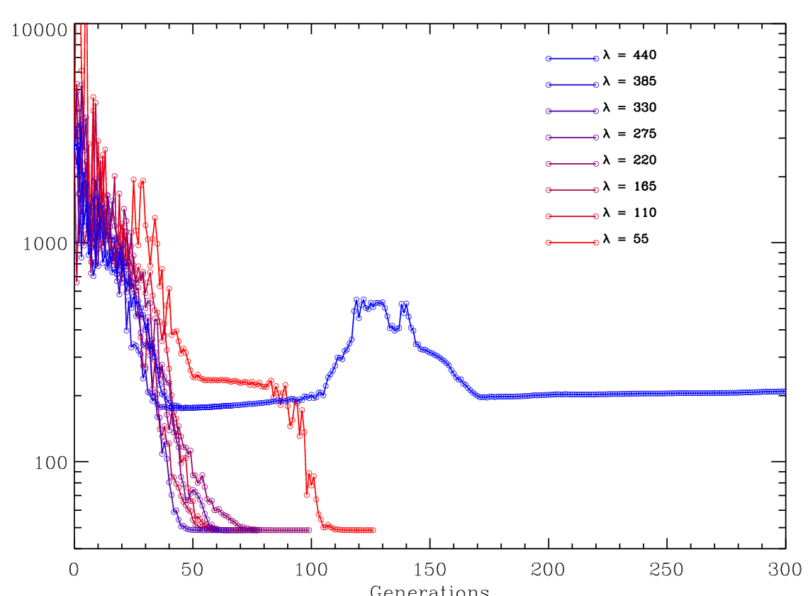
In this section, we compare the performance of CMA-ES on this particular problem by changing population size and number of offspring . First, we fix the proportion of selected offspring with respect to the entire population, which is 50%, but change the population size. The evolutionary curves are shown in Fig. 6 and the number of generations for each population size is listed in Table 4.
The population size changes from 55 to 440 as the color changes from red to blue. We can see that neither the red nor the blue curve has the best performance. The red curve, which represents the case , converges to the optimal values at but it is not the fastest option. The blue curve, which represents , actually does not converge to the optimal value; it bounces back at generation 100, returns at generation 170, and then remains around . It even exhibits a gradual increase after . The curve that shows the fastest convergence represents the case , which is 30 times the total number of free parameters.
Next, we fix the population size , but change the proportion of selected offspring. The evolutionary curves are shown in Fig. 7 and the number of generation for each proportion is listed in Table 5. The color changes from red to blue as the proportion increases from 1/10 to 1/1.5. From Fig. 7, we do not see a significant difference among these cases, although the case in which converges the fastest with the minimum number of generations (64).
Finally, we test the reliability of CMA-ES on the quasar spectrum fitting problem by running the program under the default setups (, ) 100 times. The distribution of the number of generations at which the evolution terminates is represented in Fig. 8. This figure illustrates that in general the CMA-ES algorithm is reliable; about 60% of runs converge to the optimal value.
VI Conclusion and Discussion
The CMA-ES method has achieved a preliminary success in the continuum fitting problem of a typical composite quasar spectrum. In the best case, it can finish fitting a spectrum in about 1 minute under the default setups. Although this is about 5 times longer than the LMA algorithm, it is still within the acceptable time scale. The most important aspect is that the overall fitting quality is significantly improved and the optimal results do not depend on the initial parameters. It is then feasible to extend its application to more quasar spectra and more complicated cases.
The real case can be more complicated. For instance, an iron emission template (either UV or optical) can be subdivided into a number of sections and each section may have a different scale factor. For some objects, a single PL is not enough and we usually need to include another PL at Å (if covered). Because of effective exposure time, spectra may have different signal-to-noise ratio. All of these factors may complicate the fitting process. Although the task in this work is simplified, the spectrum we are using for the test is representative of the entire sample.
The fact that the theoretical reduced value () is not reached is not because of the algorithm but the model used the fit the spectrum. A single power-law may not be an accurate description to the overall spectral profile. The iron emission shape may vary with different quasars, so a single iron emission template may not be exact. The emission lines can also contribute some flux at the benchmark wavelength points so it may not be correct to only count the contribution from the continuum at these wavelength points. Another issue is the non-uniformity of the benchmark wavelength points. When selecting these wavelength points, we were trying to use as many constraints as possible. However, because the benchmark points must avoid emission lines and there is a region in which the iron emission template is not available (between 3000 Å and 3500 Å), these benchmark points are not uniformly distributed; this could affect the evaluation.
Despite these limitations, the CMA-ES produces a limit we can reach under the best fitting model we can provide. It provides an acceptable fitting of a quasar spectrum in a timely manner. Based on these results, we can further fit the emission lines seen in the spectra.




| N | Name | Expression | Free Para. | Constraint |
|---|---|---|---|---|
| 1 | Power-law (PL) | analytical | – | |
| 2 | Small Blue Bump (SBB) | analytical11The analytical form is seen in Equation 1. | ||
| 3 | UV iron emission | templates | ||
| 4 | Optical iron emission | templates | ||
| Para. | Initialization | Remarks |
|---|---|---|
| (weighted) means of parameters, including | ||
| population size | ||
| number of parents for recombination | ||
| normalized weights | ||
| variance-effectiveness | ||
| covariance matrix | ||
| time constraint for cumulation for | ||
| const for cumulation for control | ||
| learning rate for rank-one update of | ||
| learning rate for rank- update | ||
| damping for | ||
| evolution paths for | ||
| evolution paths for | ||
| expectation of | ||
| Para. | LMA | CMA-ES |
|---|---|---|
| -1.768 | -1.713 | |
| 7.147 | 6.974 | |
| 134.827 | 150.681 | |
| 1 | 0.5153 | |
| 10000 | 10001 | |
| 0.028 | 0.044 | |
| 3000 | 3000 | |
| 0.0000 | -0.0008 | |
| 0.015 | 0.015 | |
| 3000 | 3000 | |
| 0.000 | -0.0046 |
| Population | Number of |
|---|---|
| Size | Generation |
| 55 | 127 |
| 110 | 100 |
| 165 | 82 |
| 220 | 72 |
| 275 | 78 |
| 330 | 66 |
| 385 | 76 |
| 440 | NA |
| Number of | |
|---|---|
| Proportion | Generations |
| 1/10 | 101 |
| 1/7 | 81 |
| 1/6 | 94 |
| 1/5 | 82 |
| 1/4 | 69 |
| 1/3 | 64 |
| 1/2 | 72 |
| 1/1.5 | 102 |
References
- [1] Andreas Ostermeier, A. G. . N. H. 1995, Evolutionary Computation, 2, 369
- [2] Avriel, M. 1993, ACM Trans. Program. Lang. Syst., 15, 745
- [3] Banzhaf, W., Francone, F. D., Keller, R. E., & Nordin, P. 1998, Genetic programming: an introduction: on the automatic evolution of computer programs and its applications (San Francisco, CA, USA: Morgan Kaufmann Publishers Inc.)
- [4] Beyer, H.-G., & Arnold, D. V. 2006, Evolutionary Computation, 11, 19
- [5] Björck, Å. 1996, Numerical Methods for Least Squares Problems (Philadelphia: SIAM)
- [6] Hansen, & Ostermeirer. 1996, in Proceedings of the 1996 IEEE International Conference on Evolutionary Computation, 312–317
- [7] Hansen, M., & Koumoutsakos. 2003, Evolutionary Computation, 11, 1
- [8] Hansen, N., & Kern, S. 2004, in Eighth International Conference on Parallel Problem Solving from Nature PPSN VIII, Proceedings, Berlin: Springer, 282–291
- [9] Hansen, N., & Ostermeier, A. 2001, Evolutionary Computation, 9, 159
- [10] More, J. J., & Wright, S. J. 1993, Optimization Software Guide (Philadelphia, PA, USA: Society for Industrial and Applied Mathematics)
- [11] Rosenbrock, H. H. 1960, Computer J., 3, 175
- [12] Storn, R., & Price, K. 1997, Journal of Global Minimization, 11, 341