跳到论文正文
W Papers独立论文阅读器 arXiv:1312.7343 论文正文 计算阅读时间 · 0%
引用这篇论文根据当前论文元数据生成,正式投稿前建议核对。


License: arXiv.org perpetual non-exclusive license
arXiv:1312.7343v1 [cond-mat.stat-mech] 26 Dec 2013

Efficiency analysis of diffusion on T-fractals in the sense of random walks

Preprint: AIP/123-QED
Junhao Peng Email: pengjh@gzhu.edu.cn Affiliation: College of Math and Information Science, Guangzhou University, Guangzhou 510006, China. Affiliation: Key Laboratory of Mathematics and Interdisciplinary Sciences of Guangdong Higher Education Institutes, Guangzhou University, Guangzhou 510006, China    Guoai Xu Affiliation: State Key Laboratory of Networking and Switching Technology, Beijing University of Posts and Telecommunications, Beijing 100876, China
August 24, 2026
Abstract

Efficiently controlling the diffusion process is crucial in the study of diffusion problem in complex systems. In the sense of random walks with a single trap, mean trapping time(MTT) and mean diffusing time(MDT) are good measures of trapping efficiency and diffusion efficiency respectively. They both vary with the location of the node. In this paper, we study random walks on T-fractal and provided general methods to calculate the MTT for any target node and the MDT for any source node. Using the MTT and the MDT as the measure of trapping efficiency and diffusion efficiency respectively, we compare the trapping efficiency and diffusion efficiency among all nodes of T-fractal and find the best (or worst) trapping sites and the best (or worst) diffusing sites. Our results show that: the hub node of T-fractal is the best trapping site, but it is also the worst diffusing site, the three boundary nodes are the worst trapping sites, but they are also the best diffusing sites. Comparing the minimum and maximum of MTT and MDT, we found that the maximum of MTT is almost 66 times of the minimum for MTT and the maximum of MDT is almost equal to the minimum for MDT. These results show that the location of target node has big effect on the trapping efficiency, but the location of source node almost has no effect on diffusion efficiency. We also conducted numerical simulation to test the results we have derived, the results we derived are consistent with those obtained by numerical simulation.

pacs
05.40.Fb, 89.75.Hc, 05.60.Cd

I Introduction

Efficiently controlling the diffusion and transport process is crucial in the study of diffusion and transport problem in complex systems. Random walks, which can be applied as a model for diffusion and transport phenomena in complex systems, has given rise to a lot of interest in the past few years[1, 2, 3, 4, 5, 6, 7, 8]. Many problems in physics and chemistry are related to random walks on disordered media[9, 10, 11, 12].

In the sense of random walks with a single trap, a basic quantity relevant to random walks is the trapping time or mean first-passage time (MFPT), which is the expected number of steps to hit the target node(or trap) for the first time, for a walker starting from a source node. It is a quantitative indicator to characterize the transport efficiency and many other quantities can be expressed in terms of it. Locating the target node(or trap) at one special node and average the MFPTs over all the source nodes, we get mean trapping time(MTT) for the special node. Locating the source node at one special node and average the MFPTs over all the target nodes, we obtain mean diffusing time(MDT) for the special node. Both the MTT and MDT vary with the location of node and they are good measures of trapping efficiency and diffusion efficiency respectively. Comparing the MTT and MDT among all the network nodes, we can find the effects of target node location on the trapping efficiency and the effects of source node location on diffusion efficiency. The nodes which have the minimum MTT (or the maximum MTT) are best (or worst) trapping sites and the nodes which have the minimum MDT (or maximum MDT) are the best (or worst) diffusion sites.

Because the fractal structures are able to mimic a wide range of systems[13, 14, 15, 16], in the past several years, random walks on fractals, especially the MFPT on different deterministic fractals, has been extensively studied[8, 17, 19, 18, 20, 21, 22, 23, 24]. For example, the MTT for some special nodes were obtained for different fractals(or networks), such as Sierpinski gaskets[18], Apollonian network[25], pseudofractal scale-free web [26], deterministic scale-free graph[27] and some special trees[29, 30, 31, 32, 28, 33]. The global mean first-passage time (i.e. the average of MFPTs over all pairs of nodes) were obtain for some special trees [30, 31, 32, 33, 34] and dual Sierpinski gaskets[35]. The MDT were obtained for exponential treelike networks[36], scale-free Koch networks[37] and deterministic scale-free graph[38].

However, the results of MTT and MDT which were obtained are only restricted to some special nodes for the above networks and we can neither compare the MTTs(or MDTs) among all the network nodes nor analyze the effect of nodes location on the trapping efficiency and diffusion efficiency. It is still difficult to deriving the analytic solutions of the MTT for any target node and the MDT for any source node. It is also difficult to deriving the analytic solutions of MFPT for any pair of nodes.

As for T-fractal, it is a special tree, the MTT for the hub node and the GMFPT had been obtained[39, 40, 41]. The MTT for some low-generation nodes can also be derived due to the methods of Ref. [39]. But the analytic calculations of MFPT for any pair of nodes, the MTT for any target node and the MDT for any source node were still unresolved.

In this paper, we study random walks on T-fractal based on its self-similar structure and the relations between random walks and electrical networks[42, 43]. We first provided general methods for calculating the MFPT between any pair of nodes, the MTT for any target node and MDT for any source node, then calculated MFPT, the MTT and MDT for some special nodes. We also conducted numerical simulation to test the results we have derived, the results we derived are consistent with those obtained by numerical simulation. Further more, using the MTT and the MDT as the measures of trapping efficiency and diffusion efficiency respectively, we compare the trapping efficiency and diffusion efficiency among all the nodes of T-fractal and find the best (or worst) trapping sites and the best (or worst) diffusing sites. Our results show that: the hub node of T-fractal is the best trapping site, but it is also the worst diffusing site, the three boundary nodes are the worst trapping sites, but they are also the best diffusing sites.

Comparing the minimum and maximum for MTT and MDT, we found that the maximum of MTT is almost 66 times of the minimum for MTT and the maximum of MDT is almost equal to the minimum of MDT. These results show that the trap’s position has large effect on the trapping efficiency, but the position of source node has little effect on diffusion efficiency. The methods we presented can also be used to solve the problems of MFPT on other self-similar trees.

II The network model

Here, The T-fractal we considered is constructed iteratively[40]. For convenience, we call the times of iterations as the generation of the T-fractal and denote by G⁡(t)G(t) the T-fractal of generation tt. For t=0,G⁡(0)t=0,G(0) is an edge connecting two nodes. For t>0,G⁡(t)t>0,G(t) is obtained from G⁡(t−1)G(t-1) via replacing every edge in G⁡(t−1)G(t-1) by a “T” structure illustrated in FIG. 1.
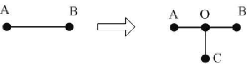
Refer to caption
Figure 1: Iterative construction method of T-fractal

The T-fractal G⁡(t)G(t) can also be constructed by another method which is shown in FIG.2: the T-fractal G⁡(t)G(t) is composed of 33 copies, called subunit, of G⁡(t−1)G(t-1) which are joined at the hub node O(i.e., nodes at the center of G⁡(t)G(t) ). According to its construction, the total number of edges for G⁡(t)G(t) is Et=3tE_{t}=3^{t} and the total number of nodes for G⁡(t)G(t) satisfies[40]

Nt=1+Et=1+3tN_{t}=1+E_{t}=1+3^{t} (1)
Refer to caption
Figure 2: Alternative construction of the T-fractal which highlights self-similarity: the T-fractal of generation tt, denoted by G⁡(t)G(t), is composed of three copies of G⁡(t−1)G(t-1) labeled as G1​(t)G_{1}(t),G2​(t)G_{2}(t),G3​(t)G_{3}(t)

III Formulation of the problem

In this paper, we study unbiased discrete random walks on the T-fractal, at each time step, the particle (walker), starting from its current location, moves to any of its nearest neighbors with equal probability. The quantity we are interested in is mean first-passage time (MFPT), which is the expected number of steps to hit the target node(or trap) for the first time, for a walker starting from a source node.

Let F⁡(x,y)F(x,y) denote the MFPT from nodes xx to yy in T-fractal G⁡(t)G(t), The sum

k⁡(x,y)=F⁡(x,y)+F⁡(x,y)k(x,y)=F(x,y)+F(x,y)

is called the commute time and the MFPT can be expressed in term of commute times[42].

F⁡(x,y)=12​{k⁡(x,y)+∑u∈G⁡(t)π⁡(u)​[k⁡(y,u)−k⁡(x,u)]}F(x,y)=\frac{1}{2}\!\left\{\!k(x,y)\!+\!\!\sum_{u\in G(t)}\!\pi(u)[k(y,u)-k(x,u)]\!\right\}\! (2)

where “u∈G⁡(t)u\in G(t)”means that uu belongs to the nodes set of G⁡(t)G(t) , π⁡(u)=du2​Et\pi(u)=\frac{d_{u}}{2E_{t}} is the stationary distribution for random walks on the T-fractal and dud_{u} is the degree of node uu.

If we view the networks under consideration as electrical networks by considering each edge to be a unit resistor and let Ψx​y\Psi_{xy} denote the effective resistance between two nodes xx and yy in the electrical networks, we have[42]

k⁡(x,y)=2​Et​Ψx​yk(x,y)=2E_{t}\Psi_{xy} (3)

where EtE_{t} is the total numbers of edges of G⁡(t)G(t). Since the T-fractals we studied are trees, the effective resistance between any two nodes is exactly the shortest-path length between the two nodes. Hence

Ψx​y=Lx​y\Psi_{xy}=L_{xy} (4)

where Lx​yL_{xy} denote the shortest path length between node xx to node yy. Thus

k⁡(x,y)=2​Et​Lx​yk(x,y)=2E_{t}L_{xy} (5)

Inserting Eq.(5) for k⁡(x,y)k(x,y) into Eq.(2),we obtain

F⁡(x,y)\displaystyle F(x,y) =\displaystyle= Et​{Lx​y+∑u∈G⁡(t)π⁡(u)​Ly​u−∑u∈G⁡(t)π⁡(u)​Lx​u}\displaystyle E_{t}\!\left\{\!L_{xy}\!+\!\!\sum_{u\in G(t)}\!\pi(u)L_{yu}\!-\!\!\sum_{u\in G(t)}\!\pi(u)L_{xu}\!\right\}\! (6)

If we average the MFPTs over all the source nodes and all target nodes, we obtain MTT and MDT respectively. That is to say, if we define

Ty\displaystyle T_{y} =\displaystyle= 1Et​∑x∈G⁡(t),x≠yF⁡(x,y)\displaystyle\frac{1}{E_{t}}\sum_{x\in G(t),x\neq y}F(x,y) (7)
Dx\displaystyle D_{x} =\displaystyle= 1Et​∑y∈G⁡(t),y≠xF⁡(x,y)\displaystyle\frac{1}{E_{t}}\sum_{y\in G(t),y\neq x}F(x,y) (8)

TyT_{y} is just the mean trapping time(MTT) for target node yy and DxD_{x} is just mean diffusing time(MDT) for source node xx. Let

Sx=∑y∈G⁡(t)Lx​yS_{x}=\sum_{y\in G(t)}{L_{xy}} (9)
Wx=∑u∈G⁡(t)π⁡(u)​Lx​u=12​Et⋅∑u∈G⁡(t)(Lx​u⋅du)W_{x}=\sum_{u\in G(t)}\pi(u)L_{xu}=\frac{1}{2E_{t}}\cdot\sum_{u\in G(t)}{(L_{xu}\cdot d_{u})} (10)
Σ=∑u∈G⁡(t)(π⁡(u)​∑x∈G⁡(t)Lx​u)\Sigma=\sum_{u\in G(t)}\left(\pi(u)\sum_{x\in G(t)}L_{xu}\right) (11)

and substitute F⁡(x,y)F(x,y) with Eq.(6) in Eqs.(7) and (8), we obtain

Ty\displaystyle T_{y} =\displaystyle= Sy+Nt⋅Wy−Σ\displaystyle S_{y}+N_{t}\cdot W_{y}-\Sigma (12)
Dx\displaystyle D_{x} =\displaystyle= Sx+Σ−Nt⋅Wx\displaystyle S_{x}+\Sigma-N_{t}\cdot W_{x} (13)

Hence, if we can calculate Σ\Sigma and Sx,WxS_{x},W_{x} for any node xx, we can calculate F⁡(x,y)F(x,y) for any two nodes (x,y)(x,y) and MTT and MDT for any node xx. Although it is difficult to calculate these quantities for general tree, we presented methods for calculating these quantities for T-fractal based on its self-similar structure. Therefore, we can calculate MTT and MDT for any node.

IV The methods for calculating MTT and MDT

IV.1 Methods for calculating SxS_{x} and WxW_{x}

For convenience, we classify the nodes of G⁡(t)G(t) into different levels. Nodes, which are introduced into the network before kk(include kk) times of iterations, are said to belong to level kk in this paper. Thus nodes which belong to level kk also belong to level k+1k+1, k+2k+2, ⋯,t\cdots,t. For example, in T-fractal of generation 33 which is shown in FIG. 3, nodes A0,B0A_{0},B_{0}, which are represented by hollow square, belong to level 00. They are also belong to level 1,2,31,2,3. Nodes represented by hollow circle belong to level 1,2,31,2,3. Nodes represented by solid square belong to level 2,32,3. Nodes represented by solid circle belong to level 33.

Refer to caption
Figure 3: The T-fractal of generation 33: levels. Hollow square, level 0,1,2,3; hollow circle, level 1,2,3; solid square, level 2,3; solid circle, level 3.

As shown in FIG. 2, The T-fractal G⁡(t)G(t) is composed of 33 subunits which are copies of G⁡(t−1)G(t-1) and G⁡(t−1)G(t-1) is also composed of 2​m+22m+2 subunits which are copies of G⁡(t−2)G(t-2) . In order to tell apart the different structures of these subunits, we classify these subunits into different levels and let Λk\Lambda_{k} denote the subunit of level k⁡(k≥0)k(k\geq 0). In this paper, G⁡(t)G(t) is said to be subunit of level 00. For any k≥0k\geq 0, the 33 subunits of Λk\Lambda_{k} are said to be subunits of level k+1k+1. Thus, any edge of G⁡(t)G(t) is a subunit of level tt and Λk\Lambda_{k} is a copy of T-fractal with generation t−kt-k.

In order to distinguish the subunits of different locations, similar to the method of Ref[39], we label the subunit Λk​(1≤k≤t)\Lambda_{k}(1\leq k\leq t) by a sequence {i1,i2,…,ik}\{i_{1},i_{2},...,i_{k}\}, where ij​((1≤j≤k))i_{j}((1\leq j\leq k)) labels its position in its father subunit Λj−1\Lambda_{j-1}. FIG. 4 shows the construction of Λk−1\Lambda_{k-1} and the relation between the value of iki_{k} and the location of subunit Λk\Lambda_{k} in Λk−1\Lambda_{k-1}: all subunit Λk\Lambda_{k} are represented by an edge, the one represented by blue edge are the subunit Λk\Lambda_{k} corresponding to value of ik=0,1,2i_{k}=0,1,2.

Refer to caption
Figure 4: Subunit represented by blue line are the subunit Λk\Lambda_{k} corresponding to value of iki_{k} below, its two boundary nodes are labeled as Ak,BkA_{k},B_{k}. Nodes labeled as Ak−1A_{k-1} in Λk−1\Lambda_{k-1} is also labeled as AkA_{k} in Λk\Lambda_{k} while ik=0i_{k}=0. Nodes labeled as Bk−1B_{k-1} in Λk−1\Lambda_{k-1} is also labeled as BkB_{k} in Λk\Lambda_{k} while ik=1i_{k}=1.

For example, in the T-fractal of generation 33 shown in FIG. 3, the subunit represented by red dotted line, which is a subunit of level 33, is labeled by a sequence {1,2,2}\{1,2,2\}.

For convenience, we label the two boundary nodes of subunit Λk\Lambda_{k} as Ak,BkA_{k},B_{k} and building mapping between boundary nodes of Λk−1\Lambda_{k-1} and those of Λk\Lambda_{k} as shown in FIG. 4. The boundary node of Λk−1\Lambda_{k-1} labeled as Ak−1A_{k-1} is also a boundary node of Λk\Lambda_{k} labeled as AkA_{k} while ik=0i_{k}=0. The boundary node of Λk−1\Lambda_{k-1} labeled as Bk−1B_{k-1} is also a boundary node of Λk\Lambda_{k} labeled as BkB_{k} while ik=1i_{k}=1.

Let

𝒮(k)≡(SAkSBk)\mathcal{S}^{(k)}\equiv\left(\begin{array}[]{c}S_{A_{k}}\\ S_{B_{k}}\end{array}\right) (14)
𝒲(k)≡(WAkWBk)\mathcal{W}^{(k)}\equiv\left(\begin{array}[]{c}W_{A_{k}}\\ W_{B_{k}}\end{array}\right) (15)

As derived in Appendix A and Appendix B, we obtain the following results.

Lemma 1

For any k>0k>0 , 𝒮(k)\mathcal{S}^{(k)} satisfy the following recursion relations

𝒮(k)=ℳik𝒮(k−1)+𝒱ikk,ik=0,1,2\hskip-28.45274pt\mathcal{S}^{(k)}=\mathcal{M}_{i_{k}}\mathcal{S}^{(k-1)}+\mathcal{V}_{i_{k}}^{k},\quad i_{k}=0,1,2 (16)

where

ℳ0=(101/21/2),𝒱0k=(0−2⋅6t−k)\mathcal{M}_{0}=\left(\begin{array}[]{cc}1&0\\ 1/2&1/2\end{array}\right),\mathcal{V}_{0}^{k}=\left(\begin{array}[]{c}0\\ -2\cdot 6^{t-k}\end{array}\right) (17)
ℳ1=(1/21/201),𝒱1k=(−2⋅6t−k0)\mathcal{M}_{1}=\left(\begin{array}[]{cc}1/2&1/2\\ 0&1\end{array}\right),\mathcal{V}_{1}^{k}=\left(\begin{array}[]{c}-2\cdot 6^{t-k}\\ 0\end{array}\right) (18)
ℳ2=(1/21/21/21/2),𝒱2k=(−2⋅6t−k(3t−3t−k+1)​2t−k)\mathcal{M}_{2}=\left(\begin{array}[]{cc}1/2&1/2\\ 1/2&1/2\end{array}\right),\mathcal{V}_{2}^{k}=\left(\begin{array}[]{c}-2\cdot 6^{t-k}\\ (3^{t}-3^{t-k+1})2^{t-k}\end{array}\right) (19)
Lemma 2

For any k>0k>0 , 𝒲(k)\mathcal{W}^{(k)} satisfy the following recursion relations

𝒲(k)=ℳik𝒲(k−1)+𝒰ikk,ik=0,1,2\mathcal{W}^{(k)}=\mathcal{M}_{i_{k}}\mathcal{W}^{(k-1)}+\mathcal{U}_{i_{k}}^{k},\quad i_{k}=0,1,2 (20)

where ℳik​(ik=0,1,2)\mathcal{M}_{i_{k}}(i_{k}=0,1,2) are given by Eqs.(17), (18), (19) and 𝒰ikk​(ik=0,1,2)\mathcal{U}_{i_{k}}^{k}(i_{k}=0,1,2) are given by

𝒰0k=(0−2t−k+13k),𝒰1k=(−2t−k+13k0)\mathcal{U}_{0}^{k}=\left(\begin{array}[]{c}0\\ -\frac{2^{t-k+1}}{3^{k}}\end{array}\right),\mathcal{U}_{1}^{k}=\left(\begin{array}[]{c}-\frac{2^{t-k+1}}{3^{k}}\\ 0\end{array}\right) (21)
𝒰2k=(−2t−k+13k2t−k​(1−13k−1))\mathcal{U}_{2}^{k}=\left(\begin{array}[]{c}-\frac{2^{t-k+1}}{3^{k}}\\ 2^{t-k}(1-\frac{1}{3^{k-1}})\end{array}\right) (22)

Using equation (16) repeatedly, we obtain

𝒮(t)\displaystyle\mathcal{S}^{(t)} =\displaystyle= ℳit​𝒮(t−1)+𝒱itt\displaystyle\mathcal{M}_{i_{t}}\mathcal{S}^{(t-1)}+\mathcal{V}_{i_{t}}^{t} (23)
=\displaystyle= ℳit​[ℳit−1​𝒮(t−2)+𝒱it−1t−1]+𝒱itt\displaystyle\mathcal{M}_{i_{t}}[\mathcal{M}_{i_{t-1}}\mathcal{S}^{(t-2)}+\mathcal{V}_{i_{t-1}}^{t-1}]+\mathcal{V}_{i_{t}}^{t}
=\displaystyle= ℳit​ℳit−1​𝒮(t−2)+ℳit​𝒱it−1t−1+𝒱itt\displaystyle\mathcal{M}_{i_{t}}\mathcal{M}_{i_{t-1}}\mathcal{S}^{(t-2)}+\mathcal{M}_{i_{t}}\mathcal{V}_{i_{t-1}}^{t-1}+\mathcal{V}_{i_{t}}^{t}
=\displaystyle= ⋯\displaystyle\cdots
=\displaystyle= ℳitℳit−1⋯ℳi1𝒮(0)\displaystyle\mathcal{M}_{i_{t}}\mathcal{M}_{i_{t-1}}\cdots\mathcal{M}_{i_{1}}\mathcal{S}^{(0)}
+∑l=1t−1ℳitℳit−1⋯ℳil+1𝒱ill+𝒱itt\displaystyle+\sum_{l=1}^{t-1}\mathcal{M}_{i_{t}}\mathcal{M}_{i_{t-1}}\cdots\mathcal{M}_{i_{l+1}}\mathcal{V}_{i_{l}}^{l}+\mathcal{V}_{i_{t}}^{t}

Similarity

𝒲(k)\displaystyle\mathcal{W}^{(k)} =\displaystyle= ℳikℳik−1⋯ℳi1𝒲(0)\displaystyle\mathcal{M}_{i_{k}}\mathcal{M}_{i_{k-1}}\cdots\mathcal{M}_{i_{1}}\mathcal{W}^{(0)} (24)
+∑l=1k−1ℳikℳik−1⋯ℳil+1𝒰ill+𝒰ikk\displaystyle+\sum_{l=1}^{k-1}\mathcal{M}_{i_{k}}\mathcal{M}_{i_{k-1}}\cdots\mathcal{M}_{i_{l+1}}\mathcal{U}_{i_{l}}^{l}+\mathcal{U}_{i_{k}}^{k}

As for 𝒮(0)\mathcal{S}^{(0)} and 𝒲(0)\mathcal{W}^{(0)}, it is easy to know

𝒮(0)=(SA0SB0)T=SA0​(11)T\displaystyle\mathcal{S}^{(0)}=(S_{A_{0}}\quad S_{B_{0}})^{T}=S_{A_{0}}(1\quad 1)^{T} (25)
𝒲(0)=(WA0WB0)T=WA0​(11)T\displaystyle\mathcal{W}^{(0)}=(W_{A_{0}}\quad W_{B_{0}})^{T}=W_{A_{0}}(1\quad 1)^{T} (26)

where (xy)T(x\quad y)^{T} is the transpose of vector (xy)(x\quad y) and SA0S_{A_{0}} and WA0W_{A_{0}} are SxS_{x} and TxT_{x} for nodes of level 00 respectively, which have been derived in Appendix C.

Noticing that any edge of G⁡(t)G(t) is a subunit of level tt, its two end nodes are just its two boundary nodes. If we know its location (i.e. the label sequence {i1,i2,…,it}\{i_{1},i_{2},...,i_{t}\}) for any edge of G⁡(t)G(t), we can exactly calculate 𝒮(t)\mathcal{S}^{(t)} and 𝒲(t)\mathcal{W}^{(t)} for its two end nodes. Hence, we can derive the expression of SxS_{x} and WxW_{x} for any node xx of G⁡(t)G(t).

IV.2 Exact calculation of Σ\Sigma

We find that

Σ=∑u∈G⁡(t)(π⁡(u)​∑x∈G⁡(t)Lx​u)=12​Et​∑u∈G⁡(t)(du​Su)\Sigma=\sum_{u\in G(t)}(\pi(u)\sum_{x\in G(t)}L_{xu})=\frac{1}{2E_{t}}\sum_{u\in G(t)}(d_{u}S_{u}) (27)

∑u∈Ω(du​Su)\sum_{u\in\Omega}(d_{u}S_{u}) is just the summation of SxS_{x} for the two end nodes of every edges of G⁡(t)G(t)(Note: for node xx which is the intersection of nn edges, SxS_{x} will be counted nn times). Because any edge of G⁡(t)G(t) is a subunit of level tt, which is in one to one correspondence with a sequence {i1,⋯,it}\{i_{1},\cdots,i_{t}\}, its two end nodes are also its two boundary nodes labeled as At,BtA_{t},B_{t}. Thus

∑u∈G⁡(t)(du​Su)=∑(∑{i1,⋯,it}𝒮(t))\sum_{u\in G(t)}(d_{u}S_{u})=\sum\left(\sum_{\{i_{1},\cdots,i_{t}\}}{\mathcal{S}^{(t)}}\right) (28)

for the right side of the equation, the second summation is run over all the subunits of level tt(i.e. let {i1,⋯,it}\{i_{1},\cdots,i_{t}\} run over all the possible values), the first summation is just add the two entries of ∑{i1,⋯,it}𝒮(t)\sum_{\{i_{1},\cdots,i_{t}\}}\mathcal{S}^{(t)} together.

Let

ℳt​o​t=ℳ0+ℳ1+ℳ2\mathcal{M}_{tot}=\mathcal{M}_{0}+\mathcal{M}_{1}+\mathcal{M}_{2} (29)
𝒱t​o​tl=𝒱0l+𝒱1l+𝒱2l\mathcal{V}_{tot}^{l}=\mathcal{V}_{0}^{l}+\mathcal{V}_{1}^{l}+\mathcal{V}_{2}^{l} (30)

we have

∑{i1,⋯,it}ℳitℳit−1⋯ℳil+1𝒱ill=3l−1ℳt​o​tt−l𝒱t​o​tl\displaystyle\sum_{\{i_{1},\cdots,i_{t}\}}\mathcal{M}_{i_{t}}\mathcal{M}_{i_{t-1}}\cdots\mathcal{M}_{i_{l+1}}\mathcal{V}_{i_{l}}^{l}=3^{l-1}\mathcal{M}_{tot}^{t-l}\mathcal{V}_{tot}^{l} (31)

Thus

∑{i1,⋯,it}𝒮(t)\displaystyle\sum_{\{i_{1},\cdots,i_{t}\}}\mathcal{S}^{(t)} =\displaystyle= ∑{i1,⋯,it}(ℳitℳit−1⋯ℳi1𝒮(0)\displaystyle\sum_{\{i_{1},\cdots,i_{t}\}}(\mathcal{M}_{i_{t}}\mathcal{M}_{i_{t-1}}\cdots\mathcal{M}_{i_{1}}\mathcal{S}^{(0)} (32)
+∑l=1t−1ℳitℳit−1⋯ℳil+1𝒱ill+𝒱itt)\displaystyle+\sum_{l=1}^{t-1}\mathcal{M}_{i_{t}}\mathcal{M}_{i_{t-1}}\cdots\mathcal{M}_{i_{l+1}}\mathcal{V}_{i_{l}}^{l}+\mathcal{V}_{i_{t}}^{t})
=\displaystyle= ℳt​o​tt​𝒮(0)+∑l=1t3l−1​ℳt​o​tt−l​𝒱t​o​tl\displaystyle\mathcal{M}_{tot}^{t}\mathcal{S}^{(0)}+\sum_{l=1}^{t}3^{l-1}\mathcal{M}_{tot}^{t-l}\mathcal{V}_{tot}^{l}

Substituting ℳi\mathcal{M}_{i} with Eqs.(17), (18) and (19) in Eq. (29), and orthogonal decomposing ℳt​o​t\mathcal{M}_{tot}, we obtain

ℳt​o​t​a​l\displaystyle\mathcal{M}_{total} =\displaystyle= (2112)\displaystyle\left(\begin{array}[]{cc}2&1\\ 1&2\end{array}\right)
=\displaystyle= (−22222222)​(1003)​(−22222222)\displaystyle\left(\begin{array}[]{cc}-\frac{\sqrt{2}}{2}&\frac{\sqrt{2}}{2}\\ \frac{\sqrt{2}}{2}&\frac{\sqrt{2}}{2}\end{array}\right)\left(\begin{array}[]{cc}1&0\\ 0&3\end{array}\right)\left(\begin{array}[]{cc}-\frac{\sqrt{2}}{2}&\frac{\sqrt{2}}{2}\\ \frac{\sqrt{2}}{2}&\frac{\sqrt{2}}{2}\end{array}\right)

Therefore

ℳt​o​t​a​lk=(−22222222)​(1003k)​(−22222222)\mathcal{M}_{total}^{k}=\left(\begin{array}[]{cc}-\frac{\sqrt{2}}{2}&\frac{\sqrt{2}}{2}\\ \frac{\sqrt{2}}{2}&\frac{\sqrt{2}}{2}\end{array}\right)\left(\begin{array}[]{cc}1&0\\ 0&{3^{k}}\end{array}\right)\left(\begin{array}[]{cc}-\frac{\sqrt{2}}{2}&\frac{\sqrt{2}}{2}\\ \frac{\sqrt{2}}{2}&\frac{\sqrt{2}}{2}\end{array}\right) (43)

Similarity

𝒱t​o​tl=(−43l−5)​6t−l\mathcal{V}_{tot}^{l}=\left(\begin{array}[]{c}-4\\ 3^{l}-5\end{array}\right)6^{t-l} (44)

Thus

ℳt​o​tt​𝒮(0)\displaystyle\mathcal{M}_{tot}^{t}\mathcal{S}^{(0)} =\displaystyle= (−22222222)​(1003t)​(−22222222)​(11)​SA0\displaystyle\!\left(\!\begin{array}[]{cc}-\frac{\sqrt{2}}{2}&\frac{\sqrt{2}}{2}\\ \frac{\sqrt{2}}{2}&\frac{\sqrt{2}}{2}\end{array}\!\right)\!\!\left(\!\begin{array}[]{cc}1&0\\ 0&{3^{t}}\end{array}\!\right)\!\!\left(\!\begin{array}[]{cc}-\frac{\sqrt{2}}{2}&\frac{\sqrt{2}}{2}\\ \frac{\sqrt{2}}{2}&\frac{\sqrt{2}}{2}\end{array}\!\right)\!\!\left(\!\begin{array}[]{c}1\\ 1\end{array}\!\right)\!S_{A_{0}}
=\displaystyle= (4⋅6t−1+3t−1)​3t​(11)\displaystyle(4\cdot 6^{t-1}+3^{t-1})3^{t}\!\left(\!\begin{array}[]{c}1\\ 1\end{array}\!\right)\!

and

∑l=1t3l−1​ℳt​o​tt−l​𝒱t​o​tl\displaystyle\sum_{l=1}^{t}3^{l-1}\mathcal{M}_{tot}^{t-l}\mathcal{V}_{tot}^{l}
=\displaystyle= ∑l=1t3l−1​6t−l​((3l−5)2​3t−l−2⋅3t−l−3l−52−2(3l−5)2​3t−l−2⋅3t−l+3l−52+2)\displaystyle\!\sum_{l=1}^{t}\!3^{l-1}6^{t-l}\!\left(\!\begin{array}[]{c}\frac{(3^{l}-5)}{2}3^{t-l}-2\cdot 3^{t-l}-\frac{3^{l}-5}{2}-2\\ \frac{(3^{l}-5)}{2}3^{t-l}-2\cdot 3^{t-l}+\frac{3^{l}-5}{2}+2\end{array}\!\right)\!

Inserting Eqs. (IV.2), (IV.2) and (148) into Eq.(32), we obtain

∑{i1,⋯,it}𝒮(t)=ℳt​o​tt​𝒮(0)+∑l=1t3l−1​ℳt​o​tt−l​𝒱t​o​tl\displaystyle\sum_{\{i_{1},\cdots,i_{t}\}}\mathcal{S}^{(t)}=\mathcal{M}_{tot}^{t}\mathcal{S}^{(0)}+\sum_{l=1}^{t}3^{l-1}\mathcal{M}_{tot}^{t-l}\mathcal{V}_{tot}^{l}
=\displaystyle= 3t⋅6t​(815+16⋅2t+310⋅6t)​(11)\displaystyle 3^{t}\cdot 6^{t}\left(\frac{8}{15}+\frac{1}{6\cdot 2^{t}}+\frac{3}{10\cdot 6^{t}}\right)\left(\begin{array}[]{c}1\\ 1\end{array}\right)

Replacing ∑{i1,⋯,it}𝒮(t)\sum_{\{i_{1},\cdots,i_{t}\}}\mathcal{S}^{(t)} with Eq.(IV.2) in Eq. (28), we get

Σ\displaystyle\Sigma =\displaystyle= 12​Et​∑u∈G⁡(t)(du​Su)\displaystyle\frac{1}{2E_{t}}\sum_{u\in G(t)}\left(d_{u}S_{u}\right) (63)
=\displaystyle= 6t​(815+16⋅2t+310⋅6t)\displaystyle 6^{t}\left(\frac{8}{15}+\frac{1}{6\cdot 2^{t}}+\frac{3}{10\cdot 6^{t}}\right)

IV.3 Examples

According to the methods presented in Sec.(IV.1) and Sec.(IV.2), we can calculate TxT_{x} and DxD_{x} for any node xx of G⁡(t)G(t). In order to explain our methods, we calculate Sx,WxS_{x},W_{x} for the three boundary nodes and the hub node labeled as A,B,C,OA,B,C,O respectilely(see FIG. 2), and then calculate the MFPT between these nodes, the MTT and MDT for these nodes.

For nodes AA and BB, according to Eqs. (148) and (150), we obtain

SA=SB=4⋅6t−1+3t−1S_{A}=S_{B}=4\cdot 6^{t-1}+3^{t-1} (64)
WA=WB=2t+13−16W_{A}=W_{B}=\frac{2^{t+1}}{3}-\frac{1}{6} (65)

For nodes OO and CC, according to Eqs. (134), (142) and (147), we have

(SOSC)\displaystyle\left(\begin{array}[]{c}S_{O}\\ S_{C}\end{array}\right) =\displaystyle= (1/21/21/21/2)​(SASB)+(−2⋅6t−k(3t−3t−k+1)⋅2t−k)\displaystyle\left(\begin{array}[]{cc}1/2&1/2\\ 1/2&1/2\end{array}\right)\left(\begin{array}[]{c}S_{A}\\ S_{B}\end{array}\right)+\left(\begin{array}[]{c}-2\cdot 6^{t-k}\\ (3^{t}-3^{t-k+1})\cdot 2^{t-k}\end{array}\right)
=\displaystyle= (2⋅6t−1+3t−14⋅6t−1+3t−1)\displaystyle\left(\begin{array}[]{c}2\cdot 6^{t-1}+3^{t-1}\\ 4\cdot 6^{t-1}+3^{t-1}\end{array}\right)

and

(WOWC)\displaystyle\left(\begin{array}[]{c}W_{O}\\ W_{C}\end{array}\right) =\displaystyle= (1/21/21/21/2)​(WAWB)+(−2t−k+13k(1−13k−1)⋅2t−k)\displaystyle\left(\begin{array}[]{cc}1/2&1/2\\ 1/2&1/2\end{array}\right)\left(\begin{array}[]{c}W_{A}\\ W_{B}\end{array}\right)+\left(\begin{array}[]{c}-\frac{2^{t-k+1}}{3^{k}}\\ (1-\frac{1}{3^{k-1}})\cdot 2^{t-k}\end{array}\right)
=\displaystyle= (2t3−162t+13−16)\displaystyle\left(\begin{array}[]{c}\frac{2^{t}}{3}-\frac{1}{6}\\ \frac{2^{t+1}}{3}-\frac{1}{6}\end{array}\right)

Thus, the MFPTs between any two nodes of AA, BB, OO and CC, which can be derived from Eq. (6), are as follows.

F⁡(A,C)\displaystyle F(A,C) =\displaystyle= F⁡(C,A)=F⁡(C,B)=F⁡(B,C)\displaystyle F(C,A)=F(C,B)=F(B,C) (90)
=\displaystyle= F⁡(B,A)=F⁡(A,B)\displaystyle F(B,A)=F(A,B)
=\displaystyle= Et​(LA​B+WB−WA)\displaystyle E_{t}(L_{AB}+W_{B}-W_{A})
=\displaystyle= 6t\displaystyle 6^{t}
F⁡(O,C)\displaystyle F(O,C) =\displaystyle= F⁡(O,A)=F⁡(O,B)\displaystyle F(O,A)=F(O,B) (91)
=\displaystyle= Et​(LO​B+WB−WO)\displaystyle E_{t}(L_{OB}+W_{B}-W_{O})
=\displaystyle= 5⋅6t−1\displaystyle 5\cdot 6^{t-1}
F⁡(C,O)\displaystyle F(C,O) =\displaystyle= F⁡(B,O)=F⁡(A,O)=6t−1\displaystyle F(B,O)=F(A,O)=6^{t-1} (92)

Insert Eqs.(63), (64), (65), (IV.3) and (IV.3) into Eq.(12), we obtain the MTT for node AA, BB, CC and OO.

TA\displaystyle T_{A} =\displaystyle= TB=TC=SA+Nt​WA−Σ\displaystyle T_{B}=T_{C}=S_{A}+N_{t}W_{A}-\Sigma (93)
=\displaystyle= 6t⋅(45+23t+1−145⋅6t+1)\displaystyle 6^{t}\cdot\left(\frac{4}{5}+\frac{2}{3^{t+1}}-\frac{14}{5\cdot 6^{t+1}}\right)
TO\displaystyle T_{O} =\displaystyle= 6t−1⋅(45+23t−145⋅6t)\displaystyle 6^{t-1}\cdot\left(\frac{4}{5}+\frac{2}{3^{t}}-\frac{14}{5\cdot 6^{t}}\right) (94)

These results are consistent with those derived in Ref. [39, 40, 41]. Insert Eqs.(63), (64), (65), (IV.3) and (IV.3) into Eq.(13), we obtain the MDT for node AA, BB, CC and OO.

DA\displaystyle D_{A} =\displaystyle= DB=DC=SA+Σ−Nt​WA\displaystyle D_{B}=D_{C}=S_{A}+\Sigma-N_{t}W_{A} (95)
=\displaystyle= 6t⋅(815+13⋅2t−1+145⋅6t+1−23t+1)\displaystyle 6^{t}\cdot\left(\frac{8}{15}+\frac{1}{3\cdot 2^{t-1}}+\frac{14}{5\cdot 6^{t+1}}-\frac{2}{3^{t+1}}\right)
DO\displaystyle D_{O} =\displaystyle= 6t⋅(815+13⋅2t−1+145⋅6t+1−13t+1)\displaystyle 6^{t}\cdot\left(\frac{8}{15}+\frac{1}{3\cdot 2^{t-1}}+\frac{14}{5\cdot 6^{t+1}}-\frac{1}{3^{t+1}}\right) (96)

We also conducted numerical simulation to test the results we have just derived, the results just derived are consistent with those obtained by numerical simulation.

V Comparison the trapping efficiency among all the nodes of T-fractal

In these section, using the MTT as the measure of trapping efficiency, we compare the trapping efficiency (i.e. the MTT) among all the nodes of T-fractal and find the best trapping sites(i.e. nodes which have the minimum MTT) and the worst trapping sites(i.e. nodes which have the maximum MTT).

First, we derive the relations of TxT_{x} for nodes of level kk and that for nodes of level k+1k+1. For any subunit of level kk as shown in FIG. 5, its two boundary nodes (i.e., AkA_{k} and BkB_{k}) are the only two nodes of level kk, its nodes of level k+1k+1 are boundary nodes of its 33 subunits of level k+1k+1(i.e., AkA_{k}, BkB_{k}, OkO_{k} and CkC_{k}). Assuming TxT_{x} for node of level kk(i.e., TAkT_{A_{k}}, TBkT_{B_{k}}) are known, we will analyze TxT_{x} for node xx of level k+1k+1(i.e., OkO_{k} and CkC_{k}).

Refer to caption
Figure 5: Labels for the 44 nodes of level k+1k+1 in Λk\Lambda_{k}.

For any k≥0k\geq 0, it is easy to obtain the following equation due to Eqs. (12), (128), (133), (142) and(147).

TOk\displaystyle T_{O_{k}} =\displaystyle= SOk−Σ+Nt​WOk\displaystyle S_{O_{k}}-\Sigma+N_{t}W_{O_{k}} (97)
=\displaystyle= 12​(SAk+SBk)−2⋅6t−k−1−Σ\displaystyle\frac{1}{2}(S_{A_{k}}+S_{B_{k}})-2\cdot 6^{t-k-1}-\Sigma
+Nt⋅[12(WAk+WBk)−2t−k3k+1]\displaystyle+N_{t}\cdot\left[\frac{1}{2}(W_{A_{k}}+W_{B_{k}})-\frac{2^{t-k}}{3^{k+1}}\right]
=\displaystyle= 12​(TAk+TBk)−4⋅6t−k−1−2t−k3k+1\displaystyle\frac{1}{2}(T_{A_{k}}+T_{B_{k}})-4\cdot 6^{t-k-1}-\frac{2^{t-k}}{3^{k+1}}

and

TCk\displaystyle\hskip-14.22636ptT_{C_{k}} =\displaystyle= SCk−Σ+Nt​WCk\displaystyle S_{C_{k}}-\Sigma+N_{t}W_{C_{k}} (98)
=\displaystyle= 12​(SAk+SBk)+(3t−3t−k)⋅2t−k−1−Σ\displaystyle\frac{1}{2}(S_{A_{k}}+S_{B_{k}})+(3^{t}-3^{t-k})\cdot 2^{t-k-1}-\Sigma
+Nt⋅{12(WAk+WBk)+(1−13k)⋅2t−k−1}\displaystyle+N_{t}\cdot\left\{\frac{1}{2}(W_{A_{k}}+W_{B_{k}})+(1-\frac{1}{3^{k}})\cdot 2^{t-k-1}\right\}
=\displaystyle= 12​(TAk+TBk)+(3t−3t−k)​2t−k+(−13k)​2t−k−1\displaystyle\!\frac{1}{2}(T_{A_{k}}\!+\!T_{B_{k}})\!+\!(3^{t}\!-\!3^{t-k})2^{t-k}\!+\!(1\!-\!\frac{1}{3^{k}})2^{t-k-1}

Note that TA0=TB0T_{A_{0}}=T_{B_{0}} and let k=0k=0 in Eqs.(97) and (98), we find

TO0<TA0=TB0=TC0\displaystyle T_{O_{0}}<T_{A_{0}}=T_{B_{0}}=T_{C_{0}} (99)

As proved in Appendix D, we find Eq.(100) holds for k≥1k\geq 1.

m​i​n​{TAk,TBk}<TOk<m​a​x​{TAk,TBk}≤TCkmin\{T_{A_{k}},T_{B_{k}}\}<T_{O_{k}}<max\{T_{A_{k}},T_{B_{k}}\}\leq T_{C_{k}} (100)

Therefore, for k≥1k\geq 1

m​i​n​{TAk,TBk}=m​i​n​{TAk,TBk,TOk,TCk}min\{T_{A_{k}},T_{B_{k}}\}=min\{T_{A_{k}},T_{B_{k}},T_{O_{k}},T_{C_{k}}\} (101)

Let Ωk\Omega_{k} denote the set for nodes of level kk and note that AkA_{k} and BkB_{k} are the only two nodes of level kk in Λk\Lambda_{k}, {Ak,Bk,Ok,Ck}\{{A_{k}},{B_{k}},{O_{k}},{C_{k}}\} represents all nodes of level k+1k+1 in Λk\Lambda_{k}, Eq.(101) implies: for any k≥1k\geq 1,

m​i​n​{Tx:x∈Ωk}=m​i​n​{Tx:x∈Ωk+1}min\{T_{x}:x\in\Omega_{k}\}=min\{T_{x}:x\in\Omega_{k+1}\} (102)

But Eqs.(99) shows

TO0=m​i​n​{Tx:x∈Ω1}<m​i​n​{Tx:x∈Ω0}T_{O_{0}}=min\{T_{x}:x\in\Omega_{1}\}<min\{T_{x}:x\in\Omega_{0}\} (103)

Thus

TO0=m​i​n​{Tx:x∈Ω1}=m​i​n​{Tx:x∈Ω}T_{O_{0}}=min\{T_{x}:x\in\Omega_{1}\}=min\{T_{x}:x\in\Omega\} (104)

Eqs.(99)and (100) also shows

TCk=m​a​x​{Tx:x∈Ωk+1}k≥0T_{C_{k}}=max\{T_{x}:x\in\Omega_{k+1}\}\qquad k\geq 0 (105)

As proved in Appendix E, we also find that: in any subunit Λk\Lambda_{k}, Eq.(106) holds for any k≥0k\geq 0.

TCk≥TCk+1T_{C_{k}}\geq T_{C_{k+1}} (106)

Therefore, in subunit Λ0\Lambda_{0} (i.e. G⁡(t)G(t))

TC0\displaystyle T_{C_{0}} =\displaystyle= m​a​x​{Tx:x∈Ω1}\displaystyle max\{T_{x}:x\in\Omega_{1}\}
≥\displaystyle\geq TCt=m​a​x​{Tx:x∈Ωt}\displaystyle T_{C_{t}}=max\{T_{x}:x\in\Omega_{t}\}

But Ωt=Ω\Omega_{t}=\Omega and C0∈ΩC_{0}\in\Omega, we obtain

TC0=m​a​x​{Tx:x∈Ωt}=m​a​x​{Tx:x∈Ω}T_{C_{0}}=max\{T_{x}:x\in\Omega_{t}\}=max\{T_{x}:x\in\Omega\} (107)

Note:TA0=TB0=TC0T_{A_{0}}=T_{B_{0}}=T_{C_{0}} and A0,B0,C0{A_{0}},{B_{0}},{C_{0}} and O0O_{0} are also labeled as A,B,CA,B,C and OO in FIG. 2. Eq.(107) and (104) shows that node O0O_{0}, which is the hub node of G⁡(t)G(t), is best trapping site, nodes A0A_{0}, B0B_{0} and C0C_{0} , which is the three boundary nodes of G⁡(t)G(t), are worst trapping sites.

Comparing TC0,TO0T_{C_{0}},T_{O_{0}} shown in Eqs.(93) and (94), while t→∞t\rightarrow\infty, we have

TC0≈6⋅TO0\displaystyle T_{C_{0}}\approx 6\cdot T_{O_{0}} (108)

which means that the location of target node has big effect on the trapping efficiency.

VI Comparison the diffusion efficiency among all the nodes of T-fractal

In these section, using the MDT as the measure of trapping efficiency, we compare the trapping efficiency (i.e., the MDT) among all the nodes of T-fractal and find the best trapping sites(i.e. nodes which have the minimum MTT) and the worst trapping sites(i.e. nodes which have the maximum MDT).

Similarity to the analysis of trapping efficiency, we first derive the relations of DxD_{x} for nodes of level kk and that for nodes of level k+1k+1, and then compare DxD_{x} for nodes of adjacent level.

Considering any subunit of level k⁡(k≥0)k(k\geq 0), which is shown in FIG. 5, it is easy to obtain the following equation due to Eqs. (13),(128), (133), (142) and (147).

DOk\displaystyle D_{O_{k}} =\displaystyle= SOk+Σ−Nt​WOk\displaystyle S_{O_{k}}+\Sigma-N_{t}W_{O_{k}} (109)
=\displaystyle= 12​(SAk+SBk)−2⋅6t−k−1+Σ\displaystyle\frac{1}{2}(S_{A_{k}}+S_{B_{k}})-2\cdot 6^{t-k-1}+\Sigma
−Nt⋅[12(WAk+WBk)−2t−k3k+1]\displaystyle-N_{t}\cdot\left[\frac{1}{2}(W_{A_{k}}+W_{B_{k}})-\frac{2^{t-k}}{3^{k+1}}\right]
=\displaystyle= 12​(DAk+DBk)+2t−k​3−k−1\displaystyle\frac{1}{2}(D_{A_{k}}+D_{B_{k}})+{2^{t-k}}{3^{-k-1}}

and

DCk\displaystyle D_{C_{k}} =\displaystyle= SCk+Σ−Nt​WCk\displaystyle S_{C_{k}}+\Sigma-N_{t}W_{C_{k}} (110)
=\displaystyle= 12​(SAk+SBk)+(3t−3t−k)⋅2t−k−1+Σ\displaystyle\frac{1}{2}(S_{A_{k}}+S_{B_{k}})+(3^{t}-3^{t-k})\cdot 2^{t-k-1}+\Sigma
−Nt⋅{12(WAk+WBk)+(1−3−k)⋅2t−k−1}\displaystyle-N_{t}\cdot\left\{\frac{1}{2}(W_{A_{k}}+W_{B_{k}})+(1-{3^{-k}})\cdot 2^{t-k-1}\right\}
=\displaystyle= 12​(DAk+DBk)−(1−3−k)⋅2t−k−1\displaystyle\frac{1}{2}(D_{A_{k}}+D_{B_{k}})-(1-{3^{-k}})\cdot 2^{t-k-1}

Note that DA0=DB0D_{A_{0}}=D_{B_{0}} and let k=0k=0 in Eqs.(109) and (110), we find

DO0>DA0=DB0=DC0\displaystyle D_{O_{0}}>D_{A_{0}}=D_{B_{0}}=D_{C_{0}} (111)

As proved in Appendix F, we find Eq.(112) holds for k≥1k\geq 1.

DOk≤m​i​n​{DAk,DBk}<DOk<m​a​x​{DAk,DBk}D_{O_{k}}\!\leq\!min\{D_{A_{k}},D_{B_{k}}\}\!<\!D_{O_{k}}\!<\!max\{D_{A_{k}},D_{B_{k}}\} (112)

Therefore, for k≥1k\geq 1, we have

m​a​x​{DAk,DBk}=m​a​x​{DAk,DBk,DOk,DCk}max\{D_{A_{k}},D_{B_{k}}\}=max\{D_{A_{k}},D_{B_{k}},D_{O_{k}},D_{C_{k}}\} (113)

Because AkA_{k} and BkB_{k} are the only two nodes of level kk in Λk\Lambda_{k} and {Ak,Bk,Ok,Ck}\{{A_{k}},{B_{k}},{O_{k}},{C_{k}}\} represents all nodes of level k+1k+1 in Λk\Lambda_{k}, Eqs.(113) implies: for any k≥1k\geq 1

m​a​x​{Dx:x∈Ωk}=m​a​x​{Dx:x∈Ωk+1}max\{D_{x}:x\in\Omega_{k}\}=max\{D_{x}:x\in\Omega_{k+1}\} (114)

But Eqs.(111) leads to

DO0=m​a​x​{Dx:x∈Ω1}>m​i​n​{Dx:x∈Ω0}D_{O_{0}}=max\{D_{x}:x\in\Omega_{1}\}>min\{D_{x}:x\in\Omega_{0}\} (115)

Thus

DO0=m​a​x​{Dx:x∈Ω1}=m​a​x​{Dx:x∈Ω}D_{O_{0}}=max\{D_{x}:x\in\Omega_{1}\}=max\{D_{x}:x\in\Omega\} (116)

Eqs.(111)and (112) also shows

DCk=m​i​n​{Tx:x∈Ωk+1}k≥0D_{C_{k}}=min\{T_{x}:x\in\Omega_{k+1}\}\qquad k\geq 0 (117)

As proved in Appendix G, we also find that: in any subunit Λk\Lambda_{k}, Eq.(118) holds for any k≥0k\geq 0.

DCk≤DCk+1D_{C_{k}}\leq D_{C_{k+1}} (118)

Therefore

DC0=m​i​n​{Tx:x∈Ω}D_{C_{0}}=min\{T_{x}:x\in\Omega\} (119)

Note: DA0=DB0=DC0D_{A_{0}}=D_{B_{0}}=D_{C_{0}} and A0,B0,C0{A_{0}},{B_{0}},{C_{0}} and O0O_{0} are also labeled as A,B,CA,B,C and OO in FIG. 2. Eq.(116) and (119) shows that node O0O_{0} is worst diffusion site, nodes A0A_{0}, B0B_{0} and C0C_{0} are best diffusion sites.

Comparing DC0,DO0D_{C_{0}},D_{O_{0}} shown in Eqs. (95) and (96), while t→∞t\rightarrow\infty, we have

DA0≈DO0\displaystyle D_{A_{0}}\approx D_{O_{0}} (120)

which means that the location of source node almost has no effect on diffusion efficiency.

VII Conclusion

In this paper,we study unbiased discrete random walks on the T-fractal, Our effort is focused on the MFPT. We present new methods to calculate the MFPT for any pair of nodes, the mean trapping time(MTT) for any target node and the mean diffusing time(MDT) for any source node. Using the MTT and the MDT as the measures of trapping efficiency and diffusion efficiency respectively, we compare the trapping efficiency and diffusion efficiency among all nodes of T-fractal and find the best (or worst) trapping sites and the best ( or worst) diffusing sites which have the minimum MDT (or maximum MDT). Our results show that: the hub node of T-fractal is the best trapping site, but it is also the worst diffusing site, the three boundary nodes are the worst trapping sites, but they are also the best diffusing sites. The methods we present can also be used to solve the problems of MFPT on other self-similar trees.

Acknowledgements.
The authors are grateful to the anonymous referees for their valuable comments and suggestions. This work was supported by the scientific research program of Guangzhou municipal colleges and universities under Grant No. 2012A022.

Appendix A Proof of Lemma 1

Considering any subunit of level k−1k-1 as shown in FIG. 6, it is composed of three subunits of level kk. It is also connected with other part of the T-fractal by its two boundary nodes (i.e. A and B in FIG. 6). In this subunit, the two boundary nodes are the only two nodes of level k−1k-1, its nodes of level kk are boundary nodes of its 33 subunits of level kk(i.e., AA, BB, OO and CC in FIG. 6). Assuming SxS_{x} for node of level k−1k-1(i.e., SAS_{A}, SBS_{B}) is known, we will analyze SxS_{x} for node xx of level kk(i.e., OO and CC).

Refer to caption
Figure 6: Construction for subunit Λk−1\Lambda_{k-1}: it is composed of three subunits of level kk labeled as G1G_{1},G2G_{2},G3G_{3} (oval with solid line in the figure), The subunit labeled as G4G_{4} denote the the rest part of the T-fractal G⁡(t)G(t) except for the subunit Λk−1\Lambda_{k-1} (oval with dotted line in the figure).

For simplify, let denote

Sx​(i)=∑y∈GiLy​xi=1,2,3,4S_{x}(i)=\sum_{y\in G_{i}}{L_{yx}}\qquad\qquad i=1,2,3,4 (121)

Thus

Sx=Sx​(1)+Sx​(2)+Sx​(3)+Sx​(4)−2​Lx​OS_{x}=S_{x}(1)+S_{x}(2)+S_{x}(3)+S_{x}(4)-2L_{xO} (122)

Because AA and OO are the two boundary nodes of subunit G1G_{1}, it is easy to know SO​(1)=SA​(1)S_{O}(1)=S_{A}(1). Note that the total numbers of nodes of G1G_{1} is Nt−kN_{t-k} and for any node y∈G1y\in G_{1}, Ly​O=Ly​B−LO​BL_{yO}=L_{yB}-L_{OB}. Therefore

SO​(1)\displaystyle S_{O}(1) =\displaystyle= ∑y∈G1Ly​O\displaystyle\sum_{y\in G_{1}}{L_{yO}} (123)
=\displaystyle= ∑y∈G1(Ly​B−LO​B)\displaystyle\sum_{y\in G_{1}}(L_{yB}-L_{OB})
=\displaystyle= SB−Nt−k​LO​B\displaystyle S_{B}-N_{t-k}L_{OB}

Thus

SO​(1)\displaystyle S_{O}(1) =\displaystyle= 12​[SA​(1)+SB​(1)−Nt−k​LB​O]\displaystyle\frac{1}{2}[S_{A}(1)+S_{B}(1)-N_{t-k}L_{BO}] (124)

By symmetry, we have

SO​(2)\displaystyle S_{O}(2) =\displaystyle= 12​[SA​(2)+SB​(2)−Nt−k​LA​O]\displaystyle\frac{1}{2}[S_{A}(2)+S_{B}(2)-N_{t-k}L_{AO}] (125)

For any node y∈G3y\in G_{3}, Ly​O=Ly​B−LO​BL_{yO}=L_{yB}-L_{OB} and Ly​O=Ly​A−LO​AL_{yO}=L_{yA}-L_{OA}. Note that LO​A=LO​BL_{OA}=L_{OB}, we have

Ly​O=12​(Ly​A+Ly​B)−LO​AL_{yO}=\frac{1}{2}(L_{yA}+L_{yB})-L_{OA}

Therefore

SO​(3)\displaystyle S_{O}(3) =\displaystyle= ∑y∈G3Ly​O\displaystyle\sum_{y\in G_{3}}{L_{yO}} (126)
=\displaystyle= ∑y∈G3[12​(Ly​A+Ly​B)−LO​A]\displaystyle\sum_{y\in G_{3}}[\frac{1}{2}(L_{yA}+L_{yB})-L_{OA}]
=\displaystyle= 12​[SA​(3)+SB​(3)]−Nt−k​LA​O\displaystyle\frac{1}{2}[S_{A}(3)+S_{B}(3)]-N_{t-k}L_{AO}

For any node y∈G4y\in G_{4}, Ly​O=12​(Ly​A+Ly​B)L_{yO}=\frac{1}{2}(L_{yA}+L_{yB}). Therefore

SO​(4)=12​[SA​(4)+SB​(4)]\displaystyle S_{O}(4)=\frac{1}{2}[S_{A}(4)+S_{B}(4)] (127)

Note that Λk\Lambda_{k} is a copy of G⁡(t−k)G(t-k), one gets LA​O=LB​O=LC​O=2t−kL_{AO}=L_{BO}=L_{CO}=2^{t-k} and Nt−k=3t−k+1N_{t-k}=3^{t-k}+1, thus

SO\displaystyle S_{O} =\displaystyle= SO​(1)+SO​(2)+SO​(3)+SO​(4)\displaystyle S_{O}(1)+S_{O}(2)+S_{O}(3)+S_{O}(4) (128)
=\displaystyle= 12​[SA​(1)+SA​(2)+SA​(3)+SA​(4)−2​LA​O]\displaystyle\frac{1}{2}[S_{A}(1)+S_{A}(2)+S_{A}(3)+S_{A}(4)-2L_{AO}]
+12​[SB​(1)+SB​(2)+SB​(3)+SB​(4)−2​LB​O]\displaystyle+\frac{1}{2}[S_{B}(1)+S_{B}(2)+S_{B}(3)+S_{B}(4)-2L_{BO}]
−2​(Nt−k−1)​LB​O\displaystyle-2(N_{t-k}-1)L_{BO}
=\displaystyle= 12​(SA+SB)−2⋅6t−k\displaystyle\frac{1}{2}(S_{A}+S_{B})-2\cdot 6^{t-k}

Similarly

SC​(1)\displaystyle S_{C}(1) =\displaystyle= SO​(1)+Nt−k​LO​C\displaystyle S_{O}(1)+N_{t-k}L_{OC} (129)
SC​(2)\displaystyle S_{C}(2) =\displaystyle= SO​(2)+Nt−k​LO​C\displaystyle S_{O}(2)+N_{t-k}L_{OC} (130)
SC​(3)\displaystyle S_{C}(3) =\displaystyle= SO​(3)\displaystyle S_{O}(3) (131)
SC​(4)\displaystyle S_{C}(4) =\displaystyle= SO​(4)+[Nt−3​Nt−k+2]​LO​C\displaystyle S_{O}(4)+[N_{t}-3N_{t-k}+2]L_{OC} (132)

Thus

SC\displaystyle S_{C} =\displaystyle= SC​(1)+SC​(2)+SC​(3)+SC​(4)−2​LO​C\displaystyle S_{C}(1)+S_{C}(2)+S_{C}(3)+S_{C}(4)-2L_{OC} (133)
=\displaystyle= [SO​(1)+SO​(2)+SO​(3)+SO​(4)]+[Nt−Nt−k]​LO​C\displaystyle[S_{O}(1)\!+\!S_{O}(2)\!+\!S_{O}(3)\!+\!S_{O}(4)]\!+\![N_{t}\!-\!N_{t-k}]L_{OC}
=\displaystyle= SO+[Nt−Nt−k]​LO​C\displaystyle S_{O}+[N_{t}-N_{t-k}]L_{OC}
=\displaystyle= 12​(SA+SB)+[Nt−3​Nt−k+2]​LO​C\displaystyle\frac{1}{2}(S_{A}+S_{B})+[N_{t}-3N_{t-k}+2]L_{OC}
=\displaystyle= 12​(SA+SB)+(3t−3t−k+1)⋅2t−k\displaystyle\frac{1}{2}(S_{A}+S_{B})+(3^{t}-3^{t-k+1})\cdot 2^{t-k}

Eqs.(128), (133) can be rewritten as a linear system

(SOSC)=(1/21/21/21/2)​(SASB)+(−2⋅6t−k(3t−3t−k+1)⋅2t−k)\left(\begin{array}[]{c}S_{O}\\ S_{C}\end{array}\right)\!=\!\!\left(\!\begin{array}[]{cc}1/2&1/2\\ 1/2&1/2\end{array}\!\right)\!\!\left(\!\begin{array}[]{c}S_{A}\\ S_{B}\end{array}\!\right)\!+\!\left(\!\begin{array}[]{c}-2\cdot 6^{t-k}\\ (3^{t}-3^{t-k+1})\cdot 2^{t-k}\end{array}\!\right)\! (134)

We label the two boundary nodes of Λk\Lambda_{k} as Ak,BkA_{k},B_{k} and building mappings between boundary nodes of Λk−1\Lambda_{k-1} and boundary nodes of Λk\Lambda_{k}, which are shown in FIG. 4.

For example, for ik=2i_{k}=2, we have the following equivalence relation.

Ak−1≡A,Bk−1≡B,Ak≡O,Bk≡CA_{k-1}\equiv A,B_{k-1}\equiv B,A_{k}\equiv O,B_{k}\equiv C

Let 𝒮(k)≡(SA⁡(k)SB⁡(k))T\mathcal{S}^{(k)}\equiv(S_{A(k)}\quad S_{B(k)})^{T}, Eqs.(134) can be rewritten as

𝒮(k)=(1/21/21/21/2)​𝒮(k−1)+(−2⋅6t−k(3t−3t−k+1)⋅2t−k)\mathcal{S}^{(k)}=\left(\begin{array}[]{cc}1/2&1/2\\ 1/2&1/2\end{array}\right)\mathcal{S}^{(k-1)}+\left(\begin{array}[]{c}-2\cdot 6^{t-k}\\ (3^{t}-3^{t-k+1})\cdot 2^{t-k}\end{array}\right) (135)

Therefore, Eq. (16) holds for ik=2i_{k}=2.

Similarly, we can verify that Eq. (16) holds for ik=0,1i_{k}=0,1.

Appendix B Proof of Lemma 2

Considering any subunit of level k−1k-1 as shown in FIG. 6, assuming WxW_{x} for nodes of level k−1k-1 (i.e. WAW_{A}, WBW_{B}) is known, we will analyze WxW_{x} for node xx of level kk (i.e. WOW_{O}, WCW_{C}). Let

Wx​(i)=12​Et⋅∑y∈Gi(Lx​y⋅dy)i=1,2,3,4W_{x}(i)=\frac{1}{2E_{t}}\cdot\sum_{y\in G_{i}}{(L_{xy}\cdot d_{y})}\qquad\qquad i=1,2,3,4 (136)

Note: the degree for nodes which is the intersection of these subgraph were counted respectively in every subgraph. For example the degree of node OO is 11 (not 33 ) in subgraph G1G_{1}, G2G_{2}, G3G_{3}. Thus

Wx=Wx​(1)+Wx​(2)+Wx​(3)+Wx​(4)W_{x}=W_{x}(1)+W_{x}(2)+W_{x}(3)+W_{x}(4) (137)

Similar to the analysis of SOS_{O}, we find

WO​(1)\displaystyle W_{O}(1) =\displaystyle= 12​[WA​(1)+WB​(1)−Et−kEt​LB​O]\displaystyle\frac{1}{2}[W_{A}(1)+W_{B}(1)-\frac{E_{t-k}}{E_{t}}L_{BO}] (138)
WO​(2)\displaystyle W_{O}(2) =\displaystyle= 12​[WA​(2)+WB​(2)−Et−kEt​LA​O]\displaystyle\frac{1}{2}[W_{A}(2)+W_{B}(2)-\frac{E_{t-k}}{E_{t}}L_{AO}] (139)
WO​(3)\displaystyle W_{O}(3) =\displaystyle= 12​[WA​(3)+WB​(3)]−Et−kEt​LC​O\displaystyle\frac{1}{2}[W_{A}(3)+W_{B}(3)]-\frac{E_{t-k}}{E_{t}}L_{CO} (140)
WO​(4)\displaystyle W_{O}(4) =\displaystyle= 12​[WA​(4)+WB​(4)]\displaystyle\frac{1}{2}[W_{A}(4)+W_{B}(4)] (141)

Thus

WO\displaystyle W_{O} =\displaystyle= WO​(1)+WO​(2)+WO​(3)+WO​(4)\displaystyle W_{O}(1)+W_{O}(2)+W_{O}(3)+W_{O}(4) (142)
=\displaystyle= 12​[WA​(1)+WA​(2)+WA​(3)+WA​(4)]\displaystyle\frac{1}{2}[W_{A}(1)+W_{A}(2)+W_{A}(3)+W_{A}(4)]
+12​[WB​(1)+WB​(2)+WB​(3)+WB​(4)]\displaystyle+\frac{1}{2}[W_{B}(1)+W_{B}(2)+W_{B}(3)+W_{B}(4)]
−2​Et−kEt​LA​O\displaystyle-2\frac{E_{t-k}}{E_{t}}L_{AO}
=\displaystyle= 12​(WA+WB)−2t−k+13k\displaystyle\frac{1}{2}(W_{A}+W_{B})-\frac{2^{t-k+1}}{3^{k}}

Similarly

WC​(1)\displaystyle W_{C}(1) =\displaystyle= WO​(1)+Et−kEt​LC​O\displaystyle W_{O}(1)+\frac{E_{t-k}}{E_{t}}L_{CO} (143)
WC​(2)\displaystyle W_{C}(2) =\displaystyle= WO​(2)+Et−kEt​LC​O\displaystyle W_{O}(2)+\frac{E_{t-k}}{E_{t}}L_{CO} (144)
WC​(3)\displaystyle W_{C}(3) =\displaystyle= WO​(3)\displaystyle W_{O}(3) (145)
WC​(4)\displaystyle W_{C}(4) =\displaystyle= WO​(4)+Et−Et−k+1Et​LC​O\displaystyle W_{O}(4)+\frac{E_{t}-E_{t-k+1}}{E_{t}}L_{CO} (146)

But Et−k+1=3​Et−kE_{t-k+1}=3E_{t-k} and one gets

WC\displaystyle W_{C} =\displaystyle= WC​(1)+WC​(2)+WC​(3)+WC​(4)\displaystyle W_{C}(1)+W_{C}(2)+W_{C}(3)+W_{C}(4) (147)
=\displaystyle= [WO​(1)+WO​(2)+WO​(3)+WO​(4)]\displaystyle[W_{O}(1)+W_{O}(2)+W_{O}(3)+W_{O}(4)]
+Et−Et−kEt​LC​O\displaystyle+\frac{E_{t}-E_{t-k}}{E_{t}}L_{CO}
=\displaystyle= WO+Et−Et−kEt​LC​O\displaystyle W_{O}+\frac{E_{t}-E_{t-k}}{E_{t}}L_{CO}
=\displaystyle= 12​(WA+WB)+(1−13k−1)⋅2t−k\displaystyle\frac{1}{2}(W_{A}+W_{B})+(1-\frac{1}{3^{k-1}})\cdot 2^{t-k}

Similar to Appendix A, if we label the two boundary nodes of Λk\Lambda_{k} as Ak,BkA_{k},B_{k} and let 𝒲(k)≡(WA⁡(k)WB⁡(k))T\mathcal{W}^{(k)}\equiv(W_{A(k)}\quad W_{B(k)})^{T}, we can verify Eq. (20) holds for ik=0,1,2i_{k}=0,1,2.

Appendix C Derivation of SA0S_{A_{0}} and WA0W_{A_{0}}

A0A_{0} is one of the two nodes of level 00 (i.e., A, B in FIG. 2), it is also one of the two boundary nodes of G⁡(t)G(t). In order to tell the difference of SA0S_{A_{0}} (and WA0W_{A_{0}} ) for the T-fractal of different generation tt, let SAtS_{A}^{t} and WAtW_{A}^{t} denote the SA0S_{A_{0}} and WA0W_{A_{0}} in T-fractal of generation tt. It is easy to know SA0=1S_{A}^{0}=1 and WA0=12W_{A}^{0}=\frac{1}{2}. For t≥1t\geq 1, according to the self-similar structure shown in FIG. 2, SAtS_{A}^{t} satisfies the following recursion relation.

SAt=SAt−1+[SAt−1+(Nt−1−1)​LB​O]+[SAt−1+(Nt−1−1)​LC​O]S_{A}^{t}=S_{A}^{t-1}\!+\![S_{A}^{t-1}\!+\!(N_{t-1}-1)L_{BO}]\!+\![S_{A}^{t-1}\!+\!(N_{t-1}-1)L_{CO}]

For the right side of the equation, the first item represents the summation for shortest path length between node AA and nodes in the subunit G1​(t)G_{1}(t), the second item represents the summation for shortest path length between node AA and nodes in the subunit G2​(t)G_{2}(t), the third item represents the summation for shortest path length between node AA and nodes in the subunit G3​(t)G_{3}(t). Note that LB​O=LC​O=2t−1L_{BO}=L_{CO}=2^{t-1} and Nt−1=3t−1+1N_{t-1}=3^{t-1}+1, we have

SA0=SAt\displaystyle S_{A_{0}}=S_{A}^{t} =\displaystyle= 3​SAt−1+2⋅6t−1\displaystyle 3S_{A}^{t-1}+2\cdot 6^{t-1} (148)
=\displaystyle= 32​SAt−2+6t−1+2⋅6t−1\displaystyle 3^{2}S_{A}^{t-2}+6^{t-1}+2\cdot 6^{t-1}
=\displaystyle= ⋯\displaystyle\cdots
=\displaystyle= 3t​SA0+2⋅6t−1​[2t−1+⋯+2−1+1]\displaystyle 3^{t}S_{A}^{0}+2\cdot 6^{t-1}[2^{t-1}+\cdots+2^{-1}+1]
=\displaystyle= 4⋅6t−1+3t−1\displaystyle 4\cdot 6^{t-1}+3^{t-1}

Similarity, we find that WAtW_{A}^{t} satisfies the following recursion relation.

WAt\displaystyle W_{A}^{t} =\displaystyle= 12​Et​∑y∈G⁡(t)(LA​y⋅dy)\displaystyle\frac{1}{2E_{t}}\sum_{y\in G(t)}({L_{Ay}\cdot d_{y}}) (149)
=\displaystyle= 12​Et{∑y∈G1​(t)LA​ydy+∑y∈G2​(t)LA​ydy\displaystyle\frac{1}{2E_{t}}\left\{\sum_{y\in G_{1}(t)}{L_{Ay}d_{y}}+\sum_{y\in G_{2}(t)}{L_{Ay}d_{y}}\right.
+∑y∈G3​(t)LA​ydy}\displaystyle+\left.\sum_{y\in G_{3}(t)}{L_{Ay}d_{y}}\right\}
=\displaystyle= WAt−1+2t3\displaystyle W_{A}^{t-1}+\frac{2^{t}}{3}

Hence

WA0=WAt\displaystyle W_{A_{0}}=W_{A}^{t} =\displaystyle= WAt−1+2t3\displaystyle W_{A}^{t-1}+\frac{2^{t}}{3} (150)
=\displaystyle= WAt−2+2t−13+2t3\displaystyle W_{A}^{t-2}+\frac{2^{t-1}}{3}+\frac{2^{t}}{3}
=\displaystyle= ⋯\displaystyle\cdots
=\displaystyle= WA0+23+223+⋯+2t3\displaystyle W_{A}^{0}+\frac{2}{3}+\frac{2^{2}}{3}+\cdots+\frac{2^{t}}{3}
=\displaystyle= 2t+13−16\displaystyle\frac{2^{t+1}}{3}-\frac{1}{6}

Appendix D Proof of Eq.(100)

For any k≥1k\geq 1, according the following mappings for nodes of Λk\Lambda_{k} and Λk+1\Lambda_{k+1}

{Ak+1≡Ak,Bk+1≡Okik+1=0Ak+1≡Ok,Bk+1≡Bkik+1=1Ak+1≡Ok,Bk+1≡Ckik+1=2\displaystyle\left\{\begin{array}[]{ll}A_{k+1}\equiv A_{k},B_{k+1}\equiv O_{k}&i_{k+1}=0\\ A_{k+1}\equiv O_{k},B_{k+1}\equiv B_{k}&i_{k+1}=1\\ A_{k+1}\equiv O_{k},B_{k+1}\equiv C_{k}&i_{k+1}=2\end{array}\right.

we have

TBk+1−TAk+1={TOk−TAkik+1=0TBk−TOkik+1=1TCk−TOkik+1=2\displaystyle T_{B_{k+1}}\!-\!T_{A_{k+1}}\!=\!\!\left\{\!\begin{array}[]{ll}T_{O_{k}}-T_{A_{k}}&i_{k+1}=0\\ T_{B_{k}}-T_{O_{k}}&i_{k+1}=1\\ T_{C_{k}}-T_{O_{k}}&i_{k+1}=2\end{array}\right.

Replacing TOkT_{O_{k}} and TCkT_{C_{k}} with Eqs.(97), (98)respectively, we have

TBk+1−TAk+1\displaystyle T_{B_{k+1}}\!-\!T_{A_{k+1}}
=\displaystyle\!=\! {12​(TBk−TAk)−4⋅6t−k−1−2t−k3k+1ik+1=012​(TBk−TAk)+4⋅6t−k−1+2t−k3k+1ik+1=1(3t−3t−k−1)​2t−k+(−13k+1)​2t−k−1ik+1=2\displaystyle\!\left\{\!\begin{array}[]{ll}\frac{1}{2}(T_{B_{k}}\!-\!T_{A_{k}})\!-\!4\cdot 6^{t-k-1}\!-\!\frac{2^{t-k}}{3^{k+1}}&i_{k+1}=0\\ \frac{1}{2}(T_{B_{k}}\!-\!T_{A_{k}})\!+\!4\cdot 6^{t-k-1}\!+\!\frac{2^{t-k}}{3^{k+1}}&i_{k+1}=1\\ (3^{t}\!-\!3^{t-k-1})2^{t\!-\!k}\!+\!(1\!-\!\frac{1}{3^{k+1}})2^{t\!-\!k\!-\!1}&i_{k+1}=2\end{array}\right.

For any k≥1k\geq 1, we find that

|TBk−TAk|≥4⋅6t−k+2t−k+1​3−k\displaystyle|T_{B_{k}}-T_{A_{k}}|\geq 4\cdot 6^{t-k}+{2^{t-k+1}}{3^{-k}} (163)
|TBk−TAk|≤(3t−3t−k)​2t−k+1+(1−3−k)​2t−k\displaystyle|T_{B_{k}}-T_{A_{k}}|\leq(3^{t}-3^{t-k})2^{t-k+1}+(1-3^{-k})2^{t-k} (164)

The Eqs.(163) and (164) are proved by mathematical induction as follows.

Note that TA0=TB0T_{A_{0}}=T_{B_{0}}, let k=0k=0 in Eq. (D), we obtain

TB1−TA1\displaystyle T_{B_{1}}-T_{A_{1}} =\displaystyle= {−4⋅6t−1−2t3i1=04⋅6t−1+2t3i1=14⋅6t−1+2t3i1=2\displaystyle\left\{\begin{array}[]{ll}-4\cdot 6^{t-1}-\frac{2^{t}}{3}&i_{1}=0\\ 4\cdot 6^{t-1}+\frac{2^{t}}{3}&i_{1}=1\\ 4\cdot 6^{t-1}+\frac{2^{t}}{3}&i_{1}=2\end{array}\right.

Thus Eqs.(163) and (164) holds for k=1k=1. Assuming that Eqs.(163) and (164) hold for some k≥1k\geq 1, we will prove that Eqs.(163) and (164) also hold for k+1k+1.

According to Eq.(D), TBk+1−TAk+1T_{B_{k+1}}-T_{A_{k+1}} has 33 cases due to the different value of ik+1i_{k+1}. It is easy to verify Eqs.(163) and (164) hold for ik+1=2i_{k+1}=2 due to Eq.(D).

For ik+1=0i_{k+1}=0, substituting TBk−TAkT_{B_{k}}-T_{A_{k}} with right side of Eq.(163), we obtain

|TBk+1−TAk+1|\displaystyle\hskip 0.0pt|T_{B_{k+1}}-T_{A_{k+1}}| (169)
=\displaystyle= |12​(TBk−TAk)−4⋅6t−k−1−2t−k​3−k−1|\displaystyle\left|\frac{1}{2}(T_{B_{k}}-T_{A_{k}})\!-\!4\cdot 6^{t-k-1}-{2^{t-k}}{3^{-k-1}}\right|
≥\displaystyle\geq 12​[4⋅6t−k+2t−k+1​3−k]−4⋅6t−k−1−2t−k3−k−1\displaystyle\frac{1}{2}\left[4\cdot 6^{t-k}+{2^{t-k+1}}{3^{-k}}\right]\!-\!4\cdot 6^{t\!-\!k\!-\!1}\!-\!\frac{2^{t-k}}{3^{\!-\!k\!-\!1}}
=\displaystyle= 8⋅6t−k−1+2⋅2t−k​3−k−1\displaystyle 8\cdot 6^{t-k-1}+2\cdot{2^{t-k}}{3^{-k-1}}
>\displaystyle> 4⋅6t−k−1+2t−k​3−k−1\displaystyle 4\cdot 6^{t-k-1}+{2^{t-k}}{3^{-k-1}}

Substituting TAk−TBkT_{A_{k}}-T_{B_{k}} with right side of Eq.(164) , we have

|TBk+1−TAk+1|\displaystyle|T_{B_{k+1}}\!-\!T_{A_{k+1}}| (170)
=\displaystyle= |12​(TBk−TAk)−4⋅6t−k−1−2t−k​3−k−1|\displaystyle\left|\frac{1}{2}(T_{B_{k}}-T_{A_{k}})\!-\!4\cdot 6^{t-k-1}-{2^{t-k}}{3^{-k-1}}\right|
≤\displaystyle\leq 12[(3t−3t−k)2t−k+1+(1−3−k)2t−k]]\displaystyle\frac{1}{2}\!\left[\!(3^{t}-3^{t-k})2^{t-k+1}+(1-3^{-k})2^{t-k}\!]\right]\!
+4⋅6t−k−1+2t−k3−k−1\displaystyle\!+\!4\cdot 6^{t-k-1}+{2^{t-k}}{3^{-k-1}}
=\displaystyle= (3t−3t−k−1)​2t−k+(1−3−k−1)​2t−k−1\displaystyle(3^{t}-3^{t-k-1})2^{t-k}+(1-3^{-k-1})2^{t-k-1}

Therefore, Eqs.(163) and (164) hold for ik+1=0i_{k+1}=0.

Similarity, we can prove they both hold for ik+1=1i_{k+1}=1. Therefore, we obtain Eqs.(163) and (164) hold for all the 33 cases of TBk+1−TAk+1T_{B_{k+1}}-T_{A_{k+1}} which led to they both hold for any k≥1k\geq 1.

We now come back to prove Eq.(100). Without loss of generality, assuming TBk≥TAkT_{B_{k}}\geq T_{A_{k}}. Similar to the proof of Eq(169) and (170), we obtain

TOk−TAk\displaystyle T_{O_{k}}-T_{A_{k}} =\displaystyle= 12​(TBk−TAk)−4⋅6t−k−1−2t−k3k+1>0\displaystyle\frac{1}{2}(T_{B_{k}}-T_{A_{k}})-4\cdot 6^{t-k-1}-\frac{2^{t-k}}{3^{k+1}}>0
TBk−TOk\displaystyle T_{B_{k}}-T_{O_{k}} =\displaystyle= 12​(TBk−TAk)+4⋅6t−k−1+2t−k3k+1>0\displaystyle\frac{1}{2}(T_{B_{k}}-T_{A_{k}})+4\cdot 6^{t-k-1}+\frac{2^{t-k}}{3^{k+1}}>0

and

TBk−TCk\displaystyle T_{B_{k}}-T_{C_{k}} =\displaystyle= 12​(TBk−TAk)−(3t−3t−k)​2t−k\displaystyle\frac{1}{2}(T_{B_{k}}-T_{A_{k}})-(3^{t}-3^{t-k})2^{t-k} (171)
−(1−3−k)​2t−k−1\displaystyle-(1-3^{-k})2^{t-k-1}
≤\displaystyle\leq 12⋅[(3t−3t−k)​2t−k+1+(1−3−k)​2t−k]\displaystyle\frac{1}{2}\cdot[(3^{t}-3^{t-k})2^{t-k+1}+(1-3^{-k})2^{t-k}]
−(3t−3t−k)​2t−k−(1−3−k)​2t−k−1\displaystyle-(3^{t}-3^{t-k})2^{t-k}-(1-3^{-k})2^{t-k-1}
=\displaystyle= 0\displaystyle 0

Therefore, Eq.(100) holds while TBk≥TAkT_{B_{k}}\geq T_{A_{k}}. By symmetry, Eq.(100) holds while TBk≤TAkT_{B_{k}}\leq T_{A_{k}}.

Appendix E Proof of Eq.(106)

According to structure of Λk\Lambda_{k}, the proof can be divided into 33 cases due to the different values of ik+1i_{k+1}. Without loss of generality, assuming TBk≥TAkT_{B_{k}}\geq T_{A_{k}}.

Case I: for ik+1=0i_{k+1}=0

TCk+1\displaystyle T_{C_{k+1}} =\displaystyle= 12​(TAk+1+TBk+1)+(3t−3t−k−1)​2t−k−1\displaystyle\frac{1}{2}(T_{A_{k+1}}+T_{B_{k+1}})+(3^{t}-3^{t-k-1})2^{t-k-1}
+(1−3−k−1)​2t−k−2\displaystyle+(1-3^{-k-1})2^{t-k-2}
=\displaystyle= 12​(TAk+TOk)+(3t−3t−k−1)​2t−k−1\displaystyle\frac{1}{2}(T_{A_{k}}+T_{O_{k}})+(3^{t}-3^{t-k-1})2^{t-k-1}
+(1−3−k−1)​2t−k−2\displaystyle+(1-3^{-k-1})2^{t-k-2}
=\displaystyle= 34​TAk+14​TBk−2⋅6t−k−1−2t−k−13k+1\displaystyle\frac{3}{4}T_{A_{k}}+\frac{1}{4}T_{B_{k}}-2\cdot 6^{t-k-1}-\frac{2^{t-k-1}}{3^{k+1}}
+(3t−3t−k−1)​2t−k−1+(1−3−k−1)​2t−k−2\displaystyle+(3^{t}-3^{t-k-1})2^{t-k-1}+(1-3^{-k-1})2^{t-k-2}
=\displaystyle= 34​TAk+14​TBk+(3t−3t−k)​2t−k−1+(1−3−k)​2t−k−2\displaystyle\frac{3}{4}T_{A_{k}}\!+\!\frac{1}{4}T_{B_{k}}\!+\!(3^{t}\!-\!3^{t\!-\!k})2^{t\!-\!k\!-\!1}\!+\!(1-3^{-k})2^{t\!-\!k\!-\!2}

Therefore

TCk+1−TCk\displaystyle T_{C_{k+1}}-T_{C_{k}} (172)
=\displaystyle= −14​(TBk−TAk)+(3t−3t−k)​2t−k−1+(−3−k)​2t−k−2\displaystyle\!-\!\frac{1}{4}(T_{B_{k}}\!-\!T_{A_{k}})\!+\!(3^{t}\!-\!3^{t\!-\!k})2^{t\!-\!k\!-\!1}\!+\!(1\!-\!3^{\!-\!k})2^{t\!-\!k\!-\!2}
−(3t−3t−k)​2t−k−(1−3−k)​2t−k−1\displaystyle-(3^{t}-3^{t-k})2^{t-k}-(1-3^{-k})2^{t-k-1}
≤\displaystyle\leq −14⋅(4⋅6t−k+2t−k+13k)−(3t−3t−k)2t−k−1\displaystyle-\frac{1}{4}\cdot\left(4\cdot 6^{t-k}+\frac{2^{t-k+1}}{3^{k}}\right)-(3^{t}-3^{t-k})2^{t-k-1}
−(1−3−k)​2t−k−2\displaystyle-(1-3^{-k})2^{t-k-2}
≤\displaystyle\leq 0\displaystyle 0

Case II: for ik+1=1i_{k+1}=1

TCk+1\displaystyle T_{C_{k+1}} =\displaystyle= 12​(TBk+TOk)+(3t−3t−k−1)​2t−k−1\displaystyle\frac{1}{2}(T_{B_{k}}+T_{O_{k}})+(3^{t}-3^{t-k-1})2^{t-k-1}
+(1−3−k−1)​2t−k−2\displaystyle+(1-3^{-k-1})2^{t-k-2}
=\displaystyle= 34​TBk+14​TAk+(3t−3t−k)​2t−k−1+(−3−k)​2t−k−2\displaystyle\frac{3}{4}T_{B_{k}}\!+\!\frac{1}{4}T_{A_{k}}\!+\!(3^{t}\!-\!3^{t\!-\!k})2^{t\!-\!k\!-\!1}\!+\!(1\!-\!3^{-k})2^{t\!-\!k\!-\!2}

Hence

TCk+1−TCk\displaystyle T_{C_{k+1}}-T_{C_{k}} (173)
=\displaystyle= 14​(TBk−TAk)+(3t−3t−k)​2t−k−1+(−3−k)​2t−k−2\displaystyle\frac{1}{4}(T_{B_{k}}\!-\!T_{A_{k}})\!+\!(3^{t}\!-\!3^{t\!-\!k})2^{t\!-\!k\!-\!1}\!+\!(1\!-\!3^{\!-\!k})2^{t\!-\!k\!-\!2}
−(3t−3t−k)​2t−k−(1−3−k)​2t−k−1\displaystyle-(3^{t}-3^{t-k})2^{t-k}-(1-3^{-k})2^{t-k-1}
≤\displaystyle\leq 14⋅[(3t−3t−k)​2t−k+1+(1−3−k)​2t−k]\displaystyle\frac{1}{4}\cdot\left[(3^{t}-3^{t-k})2^{t-k+1}+(1-3^{-k})2^{t-k}\right]
−(3t−3t−k)​2t−k−1−(1−3−k)​2t−k−2\displaystyle-(3^{t}-3^{t-k})2^{t-k-1}-(1-3^{-k})2^{t-k-2}
=\displaystyle= 0\displaystyle 0

Case III: for ik+1=2i_{k+1}=2, note that Ak+1≡Ok,Bk+1≡CkA_{k+1}\equiv O_{k},B_{k+1}\equiv C_{k}. By symmetry, we have

TCk+1=TCk\displaystyle T_{C_{k+1}}=T_{C_{k}} (174)

Thus Eq.(106) holds for ik+1=0,1,2i_{k+1}=0,1,2 and Eq.(106) holds for any k≥0k\geq 0 while TBk≥TAkT_{B_{k}}\geq T_{A_{k}}. Similarity, we can prove Eq.(106) holds while TBk≤TAkT_{B_{k}}\leq T_{A_{k}}.

Appendix F Proof of Eq.(112)

According the mappings for nodes of Λk\Lambda_{k} and Λk+1\Lambda_{k+1} as shown in Eq.(D), we have

DAk+1−DBk+1\displaystyle D_{A_{k\!+\!1}}\!-\!D_{B_{k\!+\!1}} =\displaystyle\!=\! {DAk−DOkik+1=0DOk−DBkik+1=1DOk−DCkik+1=2\displaystyle\!\left\{\!\begin{array}[]{cc}D_{A_{k}}-D_{O_{k}}&i_{k+1}=0\\ D_{O_{k}}-D_{B_{k}}&i_{k+1}=1\\ D_{O_{k}}-D_{C_{k}}&i_{k+1}=2\end{array}\right.
=\displaystyle\!=\! {12​(DAk−DBk)−2t−k3k+1ik+1=012​(DAk−DBk)+2t−k3k+1ik+1=12t−k3k+1+(−13k)​2t−k−1ik+1=2\displaystyle\!\left\{\!\begin{array}[]{ll}\frac{1}{2}(D_{A_{k}}\!-\!D_{B_{k}})\!-\!\frac{2^{t-k}}{3^{k+1}}&i_{k+1}=0\\ \frac{1}{2}(D_{A_{k}}\!-\!D_{B_{k}})\!+\!\frac{2^{t-k}}{3^{k+1}}&i_{k+1}=1\\ \frac{2^{t-k}}{3^{k+1}}\!+\!(1\!-\!\frac{1}{3^{k}})2^{t-k-1}&i_{k+1}=2\end{array}\right.

For any k≥1k\geq 1, we find

|DAk−DBk|≥2t−k+1​3−k\displaystyle|D_{A_{k}}-D_{B_{k}}|\geq{2^{t-k+1}}{3^{-k}} (183)
|DAk−DBk|≤(1−3−k)​2t−k\displaystyle|D_{A_{k}}-D_{B_{k}}|\leq(1-{3^{-k}})2^{t-k} (184)

The Eqs.(183) and (184) are proved by mathematical induction as follows.

Note that DA0=DB0D_{A_{0}}=D_{B_{0}}, let k=0k=0 in Eq. (F), we obtain

|DA1−DB1|=2t3|D_{A_{1}}-D_{B_{1}}|=\frac{2^{t}}{3}

Thus Eqs.(183)and (184) hold for k=1k=1. Assuming that Eqs.(183)and (184) hold for some k≥1k\geq 1, we will prove that Eqs.(183)and (184) also hold for k+1k+1.

According to Eq.(F), DAk+1−DBk+1D_{A_{k+1}}-D_{B_{k+1}} has 33 cases due to the different value of ik+1i_{k+1} and it is easy to verify Eqs.(183) and (184) hold for the case ik+1=2i_{k+1}=2.

For ik+1=0i_{k+1}=0, substituting DAk−DBkD_{A_{k}}-D_{B_{k}} with right side of Eq.(183), we obtain

|DAk+1−DBk+1|\displaystyle|D_{A_{k+1}}-D_{B_{k+1}}| =\displaystyle= |12​(DAk−DBk)−2t−k​3−k−1|\displaystyle\left|\frac{1}{2}(D_{A_{k}}-D_{B_{k}})-{2^{t-k}}{3^{-k-1}}\right| (185)
≥\displaystyle\geq 12⋅2t−k+1​3−k−2t−k​3−k−1\displaystyle\frac{1}{2}\cdot{2^{t-k+1}}{3^{-k}}-{2^{t-k}}{3^{-k-1}}
>\displaystyle> 2t−k​3−k−1\displaystyle{2^{t-k}}{3^{-k-1}}

Substituting DBk−DAkD_{B_{k}}-D_{A_{k}} with right side of Eq.(184), we have

|DAk+1−DBk+1|\displaystyle|D_{A_{k+1}}-D_{B_{k+1}}| =\displaystyle= |12​(DAk−DBk)−2t−k​3−k−1|\displaystyle\left|\frac{1}{2}(D_{A_{k}}-D_{B_{k}})-{2^{t-k}}{3^{-k-1}}\right| (186)
≤\displaystyle\leq (1−3−k)⋅2t−k−1+2t−k​3−k−1\displaystyle(1-{3^{-k}})\cdot 2^{t-k-1}+{2^{t-k}}{3^{-k-1}}
=\displaystyle= (1−3−k−1)​2t−k−1\displaystyle(1-{3^{-k-1}})2^{t-k-1}

Therefore, Eqs.(183) and (184) hold for ik+1=0i_{k+1}=0.

Similarity, we can prove they both hold for ik+1=1i_{k+1}=1. Therefore, Eqs.(183) and (184) hold for all the 33 cases of DBk+1−DAk+1D_{B_{k+1}}-D_{A_{k+1}} which led to they both hold for any k≥1k\geq 1.

We now come back to prove Eq.(112). Without loss of generality, assuming DAk≥DBkD_{A_{k}}\geq D_{B_{k}}. Similar to the derivation of Eq.(185) and (186), we have

DAk−DOk\displaystyle D_{A_{k}}-D_{O_{k}} =\displaystyle= 12​(DAk−DBk)−2t−k​3−k−1>0\displaystyle\frac{1}{2}(D_{A_{k}}-D_{B_{k}})-{2^{t-k}}{3^{-k-1}}>0 (187)
DOk−DBk\displaystyle D_{O_{k}}-D_{B_{k}} =\displaystyle= 12​(DAk−DBk)+2t−k​3−k−1>0\displaystyle\frac{1}{2}(D_{A_{k}}-D_{B_{k}})+{2^{t-k}}{3^{-k-1}}>0 (188)

and

DCk−DBk\displaystyle D_{C_{k}}-D_{B_{k}} =\displaystyle= 12​(DAk−DBk)−(1−13k)⋅2t−k−1\displaystyle\frac{1}{2}(D_{A_{k}}-D_{B_{k}})-(1-\frac{1}{3^{k}})\cdot 2^{t-k-1} (189)
≤\displaystyle\leq 12⋅(1−13k)​2t−k−−(1−13k)⋅2t−k−1\displaystyle\frac{1}{2}\cdot(1-\frac{1}{3^{k}})2^{t-k}--(1-\frac{1}{3^{k}})\cdot 2^{t-k-1}
=\displaystyle= 0\displaystyle 0

Thus, for any k≥1k\geq 1, Eq.(112) holds while DAk≥DBkD_{A_{k}}\geq D_{B_{k}}. By symmetry, Eq.(112) also holds while DAk≤DBkD_{A_{k}}\leq D_{B_{k}}.

Appendix G Proof of Eq.(118)

Without loss of generality, assuming DAk≥DBkD_{A_{k}}\geq D_{B_{k}}. The proof of Eq.(118) is divided into 33 cases due to the different values of ik+1i_{k+1}.

Case I: for ik+1=0i_{k+1}=0

DCk+1\displaystyle D_{C_{k+1}} =\displaystyle= 12​(DAk+1+DBk+1)−(1−13k+1)​2t−k−2\displaystyle\frac{1}{2}(D_{A_{k+1}}+D_{B_{k+1}})-(1-\frac{1}{3^{k+1}})2^{t-k-2} (190)
=\displaystyle= 12​(DAk+DOk)−(1−13k+1)​2t−k−2\displaystyle\frac{1}{2}(D_{A_{k}}+D_{O_{k}})-(1-\frac{1}{3^{k+1}})2^{t-k-2}
=\displaystyle= 34​DAk+14​DBk+2t−k−13k+1−(1−13k+1)​2t−k−2\displaystyle\frac{3}{4}D_{A_{k}}+\frac{1}{4}D_{B_{k}}+\frac{2^{t-k-1}}{3^{k+1}}-(1-\frac{1}{3^{k+1}})2^{t-k-2}
=\displaystyle= 34​DAk+14​DBk+(13k−1)​2t−k−2\displaystyle\frac{3}{4}D_{A_{k}}+\frac{1}{4}D_{B_{k}}+(\frac{1}{3^{k}}-1)2^{t-k-2}

Thus

DCk+1−DCk\displaystyle D_{C_{k+1}}-D_{C_{k}} (191)
=\displaystyle= 14​(DAk−DBk)+(13k−1)​2t−k−2+(1−13k)​2t−k−1\displaystyle\frac{1}{4}(D_{A_{k}}-D_{B_{k}})+(\frac{1}{3^{k}}-1)2^{t-k-2}+(1-\frac{1}{3^{k}})2^{t-k-1}
≥\displaystyle\geq 14⋅2t−k+13k+(1−13k)​2t−k−2\displaystyle\frac{1}{4}\cdot\frac{2^{t-k+1}}{3^{k}}+(1-\frac{1}{3^{k}})2^{t-k-2}
≥\displaystyle\geq 0\displaystyle 0

Case II: for ik+1=1i_{k+1}=1

DCk+1\displaystyle D_{C_{k+1}} =\displaystyle= 12​(DOk+DBk)−(1−13k+1)​2t−k−2\displaystyle\frac{1}{2}(D_{O_{k}}+D_{B_{k}})-(1-\frac{1}{3^{k+1}})2^{t-k-2} (192)
=\displaystyle= 14​DAk+34​DBk+2t−k−13k+1−(1−13k+1)​2t−k−2\displaystyle\frac{1}{4}D_{A_{k}}+\frac{3}{4}D_{B_{k}}+\frac{2^{t-k-1}}{3^{k+1}}-(1-\frac{1}{3^{k+1}})2^{t-k-2}
=\displaystyle= 14​DAk+34​DBk+(13k−1)​2t−k−2\displaystyle\frac{1}{4}D_{A_{k}}+\frac{3}{4}D_{B_{k}}+(\frac{1}{3^{k}}-1)2^{t-k-2}

Thus

DCk+1−DCk\displaystyle D_{C_{k+1}}-D_{C_{k}} (193)
=\displaystyle= −14​(DAk−DBk)+(13k−1)​2t−k−2+(1−13k)​2t−k−1\displaystyle-\frac{1}{4}(D_{A_{k}}-D_{B_{k}})+(\frac{1}{3^{k}}-1)2^{t-k-2}+(1-\frac{1}{3^{k}})2^{t-k-1}
≥\displaystyle\geq −14​(1−13k)​2t−k+(1−13k)​2t−k−2\displaystyle-\frac{1}{4}(1-\frac{1}{3^{k}})2^{t-k}+(1-\frac{1}{3^{k}})2^{t-k-2}
=\displaystyle= 0\displaystyle 0

Case III: for ik+1=2i_{k+1}=2, note that Ak+1≡Ok,Bk+1≡CkA_{k+1}\equiv O_{k},B_{k+1}\equiv C_{k}. By symmetry, we have

DCk+1=DCk\displaystyle D_{C_{k+1}}=D_{C_{k}} (194)

Thus Eq.(118) holds for all the three case of ik+1=0,1,2i_{k+1}=0,1,2 while DAk≥DBkD_{A_{k}}\geq D_{B_{k}}. By symmetry, it also holds while DAk≤DBkD_{A_{k}}\leq D_{B_{k}}.

References

  • [1] S. Havlin and D. ben-Avraham, Adv. Phys. 36, 695(1987).
  • [2] S. Havlin and H. Weissman, J. Phys. A: Math. Gen. 19, L1021 (1986).
  • [3] B. Kahng and S. Redner, J. Phys. A: Math. Gen. 22, 887 (1989).
  • [4] A. Maritan, Phys. Rev. Lett. 62, 2845 (1989).
  • [5] A. Bar-Haim and J. Klafter, J. Chem. Phys. 109, 5187 (1998).
  • [6] A. Maritan, G. Sartoni, and A. L. Stella, Phys. Rev. Lett. 71, 1027 (1993).
  • [7] R. Rammal, G. Toulouse, De Physique Lett. 44, 13 (1983).
  • [8] J. L. Bentz, J. W. Turner, J. J. Kozak Phys. Rev. E 82, 011137 (2010).
  • [9] J. J. Kozak, Adv. Chem. Phys. 115, 245 (2000).
  • [10] S. K. Kim, J. Chem. Phys. 28, 1057 (1958).
  • [11] D. ben-Avraham and S. Havlin, Diffusion and Reactions in Fractals and Disordered Systems (Cambridge University Press, Cambridge, UK, 2004).
  • [12] A. Blumen and G. Zumofen, J. Chem. Phys. 75, 892 (1981).
  • [13] C. Song, S. Havlin and H. A. Makse, Nat. Phys. 2, 275 (2006).
  • [14] H. D. Rozenfeld, S. Havlin and D. ben-Avraham£¬ New Journal of Physics, 9 175 (2007).
  • [15] S. N. Dorogovtsev and J. F. F. Mendes, Evolution of Networks: From Biological Nets to the Internet and WWW (Oxford University Press, Oxford, 2003)
  • [16] R. Albert and A.-L. Barabási, Rev. Modern Phys. 74, 47 (2002).
  • [17] E. W. Montroll, J. Math. Phys. 10, 753 (1969).
  • [18] J. J. Kozak and V. Balakrishnan Phys. Rev. E 65, 021105 (2002).
  • [19] A. Giacometti, A. Maritan, and H. Nakanishi, J. Stat. Phys. 75, 669 (1994).
  • [20] O. Matan and S. Havlin, Phys. Rev. A 40, 6573 (1989).
  • [21] O. Bénichou, B. Meyer, V. Tejedor, and R. Voituriez, Phys. Rev. Lett. 101, 130601 (2008).
  • [22] C. P. Haynes and A. P. Roberts, Phys. Rev. E 78, 041111 (2008).
  • [23] F. Fürstenberg, M. Dolgushev, and A. Blumen, J. Chem. Phys. 138, 034904 (2013).
  • [24] D. J. Heijs, V. A. Malyshev, and J. Knoester, J. Chem. Phys. 121, 4884 (2004).
  • [25] Z. Z. Zhang, J. H. Guan, W. L. Xie, Y. Qi and S. G. Zhou, EPL 86, 10006 (2009).
  • [26] Z.Z. Zhang, Y. Qi, S.G.Zhou, W. L. Xie and J. H. Guan, Phys. Rev. E 79, 021127 (2009)
  • [27] E. Agliari, R. Burioni and A. Manzotti1, Phys. Rev. E 82, 011118 (2010).
  • [28] B. Wu, Y. Lin, Z. Z. Zhang, and G. R. Chen, J. Chem. Phys. 137, 044903 (2012).
  • [29] F. Comellas, A. Miralles, Phys. Rev. E 81, 061103 (2010).
  • [30] Z.Z. Zhang, Y. Qi, S.G.Zhou, S.Y.Gao and J.H.Guan, Phys. Rev. E 81, 016114 (2010).
  • [31] Y. Lin and Z. Z. Zhang, J. Chem. Phys., 138, 094905 (2013).
  • [32] Y. Lin, B. Wu, and Z. Z. Zhang, Phys. Rev. E 82, 031140 (2010).
  • [33] Z.Z. Zhang , Y.Lin and Y.J. Ma, J. Phys. A: Math. Theor. 44, 075102 (2011).
  • [34] Z. Z. Zhang, B. Wu, H. J. Zhang, S. G. Zhou, J. H. Guan, and Z. G. Wang, Phys. Rev. E 81, 031118 (2010).
  • [35] S. Q. Wu, Z. Z. Zhang, and G. R. Chen, Eur. Phys. J. B, 82, 91 (2011).
  • [36] Z. Z. Zhang, X. T. Li, Y. Lin, G. R. Chen, J. Stat. Mech. P08013 (2011).
  • [37] Z.Z. Zhang and S.Y.Gao, Eur. Phys. J. B 80, 209 (2011).
  • [38] E. Agliariand R. Burioni, Phys. Rev. E 80, 031125 (2009).
  • [39] B. Meyer, E. Agliari, O. Bénichou, and R. Voituriez, Phys. Rev. E 85, 026113 (2012).
  • [40] E. Agliari Phys. Rev. E 77, 011128 (2008).
  • [41] Z. Z. Zhang, Y. Lin, S. G. Zhou, B. Wu, J. H. Guan , New Journal of Physics, 11, 103043 92009).
  • [42] P. Tetali, J. Theoretical Probability, 1, 101 (1991).
  • [43] L. LOVASZ Combinatorics, Paul erdös is eighty 2, 1 (1993).

*