Modularity, Calabi-Yau geometry and 2d CFTsThanks: It is a great pleasure to thank H. Ooguri and D. Friedan for collaboration on the work described here, and T. Hartman for discussions of some of the points presented here. This work was supported by the Rutgers New High Energy Theory Center and by U.S. DOE Grants No. DOE-SC0010008, DOE-ARRA-SC0003883 and DOE-DE-SC0007897.

The conformal bootstrap is the project of constructing conformal field theories from consistency conditions imposed by conformal invariance [15, 11, 16]. Compared to other methods, its main advantage is that it does not rely on a Lagrangian description of the CFT. It makes use of the conformal symmetry of the theory by decomposing amplitudes into conformal blocks — the contributions of the irreducible representations of the conformal group. In principle it is thus possible to classify and construct all CFTs, including strongly coupled ones.

For CFTs in two dimensions, the amplitudes are subject to two types of consistency conditions. First, there is crossing symmetry. Defining the four point function

(1.1)

$$G(x):=\langle\phi(\infty)\phi(1)\phi(x)\phi(0)\rangle\ ,$$

it follows from invariance under the global conformal transformation $z\mapsto 1-z$ that $G(x)=G(1-x)$. On the other hand one can decompose $G$ into conformal blocks

(1.2)

$$G(x)=\sum_{\psi\in S}C^{2}_{\phi\phi\psi}\mathcal{F}(x)\mathcal{F}(\bar{x})\ .$$

The conformal block $\mathcal{F}$ is universal and only depends on the weights $h$ and the central charge $c$. Here $S$ is the spectrum of all primary fields that appear in the OPE of $\phi$ with itself. Crucially, $\mathcal{F}(x)\neq\mathcal{F}(1-x)$. This means that (1.2) can only be satisfied if we choose the spectrum $S$ and the three-point functions $C_{\phi\phi\psi}$ very carefully. For rational CFTs there are only a finite number of primaries, so that finding solutions is feasible. More recently, starting with [18] there has been a lot of progress also for the general case and for higher dimensions. The main ingredients for this modern bootstrap approach to work are having explicit expressions for $\mathcal{F}(x)$ and unitarity of the theory, which implies $C^{2}\geq 0$. Fixing the dimension of the external field $\phi$, this allows to deduce an upper bound for the lowest lying field in the spectrum of the OPE of $\phi$ with itself.

The second consistency condition is modular invariance for amplitudes on higher genus Riemann surfaces. In particular it requires that the partition function

(1.3)

$$Z(\tau)={\rm Tr}q^{L_{0}-c/24}\bar{q}^{\bar{L}_{0}-c/24}\qquad q=e^{2\pi i\tau}$$

is invariant under modular transformations, namely $Z(-1/\tau)=Z(\tau)$. This follows from interpreting (1.3) as the vacuum amplitude on the torus. Since this should only depend on the conformal structure $\tau\in\mathbb{H}^{+}/SL(2,\mathbb{Z})$ of the torus, it must be a modular invariant function of $\tau$. Again the representation theory of the conformal group allows us to decompose $Z$ into characters,

(1.4)

$$Z(\tau)=\sum_{h,\bar{h}\in S}N_{h,\bar{h}}\overline{\chi_{\bar{h}}(\tau)}\chi_{h}(\tau)\ ,$$

from which we can derive constraints on the spectrum $S$ and the multiplicities $N_{h,\bar{h}}$. As before, the characters $\chi$ themselves are not modular invariant, so that only special choices for the spectrum give a good partition function.

Note that for 2d CFTs crossing symmetry on the sphere and modular invariance on the torus are enough to ensure consistency of the theory [12]. We can obtain amplitudes on higher genus Riemann surfaces by gluing these two components, the consistency of this procedure being guaranteed by crossing symmetry of the 4pt functions and modular invariance of the torus 1pt functions. The situation is less clear in higher dimensions, and it is still an open question what corresponds to modular invariance then.

We will describe here the investigation [7, 9, 4] of CFTs with a gap. For such theories, other than the vacuum we do not allow for any primary with total weight less than a certain weight $\Delta_{1}$, so that $S$ is of the form

(1.5)

$$S_{\Delta_{1}}=\left\{(h,\bar{h})\,:\,h,\bar{h}\geq 0,\;h+\bar{h}\geq\Delta_{1}\right\}\ .$$

A theory which saturates the largest possible gap is called extremal. Such extremal theories could for instance arise as a holographic dual to pure gravity on $AdS_{3}$ [19]. More generally, this gives information on the structure of modular forms in the following sense.

Consider first the analog problem for meromorphic partition functions. Modular invariance means that $Z(\tau)$ is well-defined on $\mathbb{H}^{+}/SL(2,\mathbb{Z})$, which is compact. Meromorphic functions on compact spaces are determined by their poles. Since for physical reasons we know that the only pole is at $q=0$, it follows that for a holomorphic CFT with central charge $c=24k$, the largest gap is $\Delta_{1}=\frac{c}{24}+1$. Note that although one can construct such extremal partition functions for all values of $k$, it is not clear that the corresponding extremal CFTs exist.

We expect the space of non-meromorphic partition functions to be much bigger and its structure more complicated. A priori the bound on the gap will thus be weaker, and it is interesting to investigate by how much. In the first part of this review we will discuss this question.

As an aside, note that for such holomorphic theories also the crossing symmetry problem simplifies. In this case the 4pt function is meromorphic and thus determined by its poles. For an external field of weight $h_{\phi}$ the first $2h_{\phi}-1$ terms in the OPE thus fix the full 4pt function. The space of contributions to the 4pt function is thus at most $2h_{\phi}-1$ dimensional, and it is a problem in finite dimensional linear algebra to find crossing symmetric elements. In the end one finds an upper bound for the field in the internal channel of the form $h_{\psi}\leq\frac{4}{3}h_{\phi}+O(1)$, as was obtained in [2] in the context of classifying $W$-algebras. The advantage of this method is that there are no numerical computations involved, which in particular allows to go to very high values of $c$ and $h_{\phi}$. It would be interesting to extend this type of analytic approach to non-holomorphic theories.

Finally note that so far all these methods only give an upper bound for the lowest field in the spectrum. Once we are confident that we have obtained the best possible bound, we can try to reconstruct the spectrum of this extremal theory. This is done by extracting the multiplicity of the lowest primary fields, and then bootstrapping our way up the spectrum. In various contexts this type of program has been applied successfully [3, 6, 17]. For our type of problem however generically this approach fails. As we will see, we do not impose integrality of the multiplicities $N_{h,\bar{h}}$ when deriving our bounds. This means that in general the multplicities obtained for our extremal spectra will not be integral. Still in some special cases they may become integer, which would suggest strongly that there exists a corresponding CFT.

In this section we discuss how to obtain an upper bound $\Delta_{1}$ for the lowest lying primary of a general CFT of central charge $c$. A first such bound was obtained in [7], and [4] discussed how to improve on it systematically.

For simplicity choose a purely imaginary $\tau=i\beta$. Introducing the notation $\tilde{Z}=Z(\beta^{-1})$, modular invariance of the partition function can be written as

(2.1)

$$v_{0}:=-(Z_{0}-\tilde{Z}_{0})=\sum_{h,\bar{h}\in S}N_{h,\bar{h}}(Z_{h,\bar{h}}-\tilde{Z}_{h,\bar{h}})\ ,$$

where the left hand side is the contribution of the vacuum, and the right hand side the contribution of all the other primaries.

There is a very nice geometric interpretation of (2.1). Restricting to theories that have only fields of total weight $h+\bar{h}\geq\Delta_{1}$ in their spectrum $S$, the right hand side forms a convex cone $C_{\Delta_{1}}$ in the space of functions in $\beta$. Checking the existence of such a partition function reduces to checking if the vacuum contribution $v_{0}$ is in $C_{\Delta_{1}}$.

One way to check this is to search for a hyperplane $\rho$ that separates $v_{0}$ from the cone. Such a linear functional has to satisfy

(2.2)

$$\rho|_{C_{\Delta_{1}}}\geq 0\quad\textrm{and}\quad\rho(v_{0})<0\ .$$

If we can construct such a functional, then we know that there cannot be a CFT with a gap as large as $\Delta_{1}$. Our strategy will therefore be to scan as systematically as possible over the space of linear functionals, attempting to find a separating one.

To do this, let us first simplify the problem by defining a reduced partition function

(2.3)

$$\hat{Z}(\tau)=|\tau|^{1/2}|\eta(\tau)|^{2}Z(\tau)\ .$$

Note that $\hat{Z}$ is still invariant under $S$, so that we can perform our analysis with the reduced function. We are using the fact that the characters of the Virasoro algebra are essentially the $\eta$ function, which itself is modular. The reduced contribution of the primary fields is the simple monomial $\hat{Z}_{h,\bar{h}}=|\tau|^{1/2}q^{h-\gamma}\bar{q}^{\bar{h}-\gamma}$, and the vacuum contribution is $\hat{Z}_{0}=|\tau|^{1/2}|1-q|^{2}q^{-\gamma}\bar{q}^{-\gamma}$. We have introduced $\gamma=\frac{c-1}{24}$, where the -1 comes from the effective central charge of the Virasoro algebra, which we effectively removed by dividing out the $\eta$ function.

Since we are dealing with analytic functions, one way to construct linear functionals is by extracting Taylor coefficients. More precisely we can act with differential operators $\beta\partial_{\beta}$ and evaluate the result at the self-dual point $\beta=1$. The advantage of using the logarithmic derivative is that it is odd under $S$. Given such a differential operator $\mathcal{D}$ of order $n_{\mathcal{D}}$, by the simple form of $Z_{h,\bar{h}}$ we obtain a polynomial $p$,

(2.4)

$$(\mathcal{D},Z_{h,\bar{h}})=e^{-2\pi(\Delta-2\gamma)}p(\Delta)\ .$$

The positivity condition in (2.2) thus reduces to checking that $p(\Delta)\geq 0$ if $\Delta\geq\Delta_{1}$. Note that by construction both sides of (2.1) are odd under $S$. This means we can restrict to odd differential operators ${\mathcal{D}}$.

We can in fact rewrite any such polynomial in the form

(2.5)

$$p(\Delta)=\vec{\Delta}^{T}Y_{1}\vec{\Delta}+(\Delta-\Delta_{1})\vec{\Delta}^{T}Y_{2}\vec{\Delta}\ ,$$

where $\vec{\Delta}=(1,\Delta,\Delta^{2},\ldots,\Delta^{n})$ and $Y_{1,2}$ are positive semidefinite matrices.¹¹ 1 In the case here this is related to the fact that we can write any positive polynomial as a sum of squares. For polynomials in more variables the situation is more complicated, and is related to Hilbert’s 17th problem. To find a separating hyperplane as in (2.2), we thus scan over the space of semidefinite matrices $Y_{1,2}$. We need to impose some linear constraints ensuring that the corresponding polynomials actually can come from a differential operator $\mathcal{D}$, and also to fix the overall normalization of $\rho$. The goal is then to find matrices $Y_{1,2}$ which maximize $\rho(-v_{0})$. If this maximum is positive, then we have indeed found a separating hyperplane and can conclude that $\Delta_{1}$ is an upper bound for the gap of any CFT. We have thus phrased our problem as maximizing a linear objective function over a set of semidefinite matrices under a set of linear constraints. Such problems have been well studied in linear programming, and powerful numerical solvers have been developed such as SDPA [10].

We have plotted the results in figure 2, which shows how the bound $\Delta_{1}(c)$ improves as we increase the order of the differential operator $n_{\mathcal{D}}$. The original bound [7] is the case $n_{{{\mathcal{D}}}}=3$. For small $c$ the improvements are relatively small, and we seem to converge to a best possible bound very quickly. For larger $c$ we have to go to higher and higher order operators to get accurate results.

Let us discuss the asymptotic behavior for large $c$ in more detail here. The main interest for this comes from the $AdS_{3}/CFT_{2}$ correspondence, in which the limit $c\rightarrow\infty$ on the CFT side corresponds to the classical limit on the gravity side, for which semiclassical computations are appropriate. The extremal partition function we investigate here would correspond to pure gravity [19]. More generally, theories that are dual to gravity theories should have only a small number of low-lying states. It is thus reasonable to assume that to leading order they have to satisfy the same bound $\Delta_{1}$. On the other hand all such theories should contain BTZ black holes [1]. On the CFT side this means that there should be an exponential number of primary fields starting at weight $\frac{c}{12}$. This suggests that $\Delta_{1}$ should grow as $\frac{c}{12}$.

The original bound found for $n_{{{\mathcal{D}}}}=3$ grows as $\frac{c}{6}$. Figure 2 seems to suggest that the bounds from higher operators have a better asymptotic. It turns out however that for large enough $c$ they all asymptote as $\frac{c}{6}$ if we keep $n_{{{\mathcal{D}}}}$ fixed. Since figure 2 is so suggestive, it is possible that this simply an order of limit issue. That is, for a given $c$ it may be possible to find a differential operator that gives a bound whose leading behavior in $c$ is better than $\frac{c}{12}$ — our arguments simply show that the order of this operator would have to grow with $c$. This suggests that as a basis for linear functionals, finite order differential operators are not really appropriate for investigating this type of question. It would be interesting to construct a more appropriate basis, and check if the asymptotic behavior is indeed as predicted by holography.

The only thing we do know for certain is that no bound obtained in such a way can be better than the barrier $\Delta_{1}=2\gamma=\frac{c}{12}+O(1)$. This can be seen for example by comparison to the holomorphic case discussed in section 1,²² 2 To compare to the holomorphic case, note that in the results quoted here we set $c=\frac{c_{L}+c_{R}}{2}$. or also by a direct argument [5].

Let us now consider non-linear $\sigma$-models on Calabi-Yau $d$-folds. Such CFTs have more symmetry, namely extended $N=(2,2)$ superconformal symmetry. The extension comes from the holomorphic $(d,0)$ form $\Omega$, which on the CFT side leads to invariance under one unit of spectral flow. Because of the $U(1)$ $R$-symmetry of the algebra, the Cartan torus has an additional element, so that we can compute a generalized partition function

(3.1)

$$Z(\tau,\bar{\tau},z,\bar{z})={\rm Tr}\left(q^{L_{0}-c/24}\bar{q}^{\bar{L}_{0}-c/24}y^{J_{0}}\bar{y}^{\bar{J}_{0}}\right)\ ,\qquad y=e^{2\pi iz}\ .$$

We can compute the partition function for the different spin structure by taking the trace in the NS or R sector, and by inserting fermion parity operators. We will concentrate on the $(-,-)$ spin structure, that is the untwisted NS sector without any fermion number operator inserted. Under the $S$ transformation

(3.2)

$$S:(\tau,z)\mapsto(\tilde{\tau},\tilde{z})=(-1/\tau,z/\tau)\,,$$

it transforms as [8]

(3.3)

$$Z(\tau,z)=e^{-2\pi i\frac{d}{2}\frac{z^{2}}{\tau}}\,e^{2\pi i\frac{d}{2}\frac{\bar{z}^{2}}{\bar{\tau}}}\,Z(\tilde{\tau},\tilde{z})\,,$$

i.e. it is invariant up to a phase. Note that it will not transform to itself under the full modular group, but rather under $\Gamma_{\theta}$, the subgroup generated by $S$ and $T^{2}$. Using a combination of $T$ and $S$ transformations we can obtain partition functions of other spin structures.

The representation theory of the extended $N=(2,2)$ superconformal symmetry has been studied in [13]. There are $d$ short representations $\chi^{Q}$, and $d-1$ families of long representations ${\textrm{ch}}^{Q}_{h}$, labeled by their weights $h$ and $U(1)$ charges $Q$. Combining left- and right-moving short representations gives $\frac{1}{2}$-BPS states, whereas a combination of a long with a short representation give a $\frac{1}{4}$-BPS state, leading to a total partition function of the form

(3.4)

$$Z=Z_{\frac{1}{2}BPS}+Z_{\frac{1}{4}BPS}+Z_{m}\ ,$$

where $Z_{m}$ contains all the non-BPS states. Schematically, the representations of the $\sigma$-model are related to the Calabi-Yau as

	topology	$\displaystyle\leftrightarrow$	BPS states
	geometry	$\displaystyle\leftrightarrow$	non-BPS states

More precisely, the $\frac{1}{2}$BPS states are fixed by the Hodge numbers, and the $\frac{1}{4}$BPS states essentially by the elliptic genus of the manifold. In general a lot is known about the topology of CY manifolds, and hence about the BPS states of the theory. We will try to extract information about the spectrum of non-BPS states. In the end, we will give an upper bound $\Delta_{1}$ for the lowest lying non-BPS primary as a function of the Hodge numbers of the manifold.

For this analysis it is straightforward to apply the same method as in the Virasoro case. A priori it seems that the space of functions to analyze now depends on the two variables $\tau$ and $z$. However, spectral flow invariance allows us to factor out the $z$ dependence of $Z$ in terms of $\theta$-functions. More precisely, Hermite’s Lemma tells us that the space of such functions has dimension $d$ over the functions of $\tau$, and can be spanned by $d$ $\theta$-functions

(3.5)

$$f_{d}^{Q}(\tau,z)=\frac{1}{\eta(\tau)}\sum_{m\in\mathbb{Z}}q^{\frac{d}{2}(m+Q/d)^{2}}y^{d(m+Q/d)}\ .$$

The $f_{d}^{Q}$ we have picked here form a particular suitable basis because they transform linearly under the $S$ modular transformation with simple transformation matrices: Let $\mathbf{F}_{d}$ be the $d$-vector with entries $e^{\frac{i\pi dz^{2}}{2\tau}}f_{d}^{Q}$. Then [14]

(3.6)

$$\mathbf{F}_{d}(\tilde{\tau},\tilde{z})=\mathbf{S}_{d}\,\mathbf{F}_{d}(\tau,z)\,,\qquad(\mathbf{S}_{d})_{Q^{\prime}}^{Q}=d^{-\frac{1}{2}}e^{-2\pi iQQ^{\prime}/d}\,.$$

The transformation matrix $\mathbf{S}_{d}$ is unitary and its entries are just numbers. In view of (3.3), we again define a reduced partition function

(3.7)

$$\hat{Z}(\tau,z)=\left|e^{\frac{i\pi dz^{2}}{2\tau}}(-i\tau)^{1/4}\eta(\tau)\right|^{2}Z(\tau,z)\,,$$

so that $S$ modular invariance becomes simply

(3.8)

$$\hat{Z}(\tau,z)=\hat{Z}(\tilde{\tau},\tilde{z})\,.$$

Using the fact that we can express all characters in terms of $\mathbf{F}$, we can write the reduced partition function as

(3.9)

$$\hat{Z}(\tau,z)=\mathbf{F}_{d}^{\dagger}\,\mathbf{M}(\tau)\,\mathbf{F}_{d}\,,$$

where the $d\times d$ matrix $\mathbf{M}(\tau)$ is determined by the multiplicities of the various representations. Note that crucially $\mathbf{M}(\tau)$ only depends on $\tau$, and not on $z$ anymore. In some cases the expressions for $\mathbf{M}$ become very simple, and we will give explicit examples below. Modular invariance (3.8) is then equivalent to the matrix equation

(3.10)

$$\mathbf{M}(\tau)=\mathbf{S}_{d}^{\dagger}\,\mathbf{M}(\tilde{\tau})\,\mathbf{S}_{d}\,.$$

We are thus back at a variant of the bosonic modular invariance problem. Linear functionals $\rho$ are now given by $d\times d$ matrices ${\mathcal{D}}^{QQ^{\prime}}$ of differential operators

(3.11)

$${\mathcal{D}}=\mathbf{D}(\tau\partial_{\tau})$$

where $\mathbf{D}$ is a matrix of polynomials in $\tau\partial_{\tau}$ and $\bar{\tau}\partial_{\bar{\tau}}$. A matrix differential operator ${\mathcal{D}}$ acts on a matrix of functions $\mathbf{A}$ by

(3.12)

$$({\mathcal{D}},\mathbf{A})={\rm Tr}(\mathbf{D}^{\dagger}\mathbf{A})\bigr|_{\tau=i}\,.$$

We separate $\mathbf{M}$ into two parts

(3.13)

$$\mathbf{M}=\mathbf{M}_{BPS}+\mathbf{M}_{m}\,,$$

where the BPS contribution $\mathbf{M}_{BPS}$ comes from the multiplicities that are determined by the known topological properties of the Calabi-Yau manifold, that is the BPS states. The rest of the multiplicities determine $\mathbf{M}_{m}$, which due to their positivity again span a convex cone in the function space. On this cone the semidefinite condition on ${\mathcal{D}}$ is

(3.14)

$$({\mathcal{D}},\mathbf{M}_{m})\geq 0$$

for all possible multiplicities consistent with a given gap $\Delta_{1}$.

We shall restrict ourselves to the case of Calabi-Yau 3-folds here. In this case additional simplifications occur. The $\frac{1}{2}$BPS part is then given by³³ 3 For simplicity we assume here that there are no additional continuous symmetries in the theory.

(3.15)

$$Z_{\frac{1}{2}BPS}=\bar{\chi}^{0}\chi^{0}+h^{1,1}(\bar{\chi}^{1}\chi^{1}+\bar{\chi}^{-1}\chi^{-1})+h^{2,1}(\bar{\chi}^{1}\chi^{-1}+\bar{\chi}^{-1}\chi^{1})\ .$$

The elliptic genus is given by

(3.16)

$$J=(h^{1,1}-h^{2,1})\phi_{0,3/2}$$

where $\phi_{0,3/2}$ is the unique weak Jacobi form of weight 0 and index $3/2$. Rather surprisingly it turns out that in the case at hand (3.15) itself is already a weak Jacobi form once we flow to the R sector and compute the elliptic genus, i.e.

(3.17)

$$Z_{\frac{1}{2}BPS}\rightarrow J\ .$$

It follows that the $\frac{1}{4}$BPS contributions need to vanish, so that $Z_{\frac{1}{4}BPS}=0$. Note that for other dimensions $d$ one has add corrections from $\frac{1}{4}$BPS to obtain a weak Jacobi form. It would be interesting to understand this coincidence for $d=3$ more conceptually.

This allows us to reduce the matrix $\mathbf{M}$ from a $3\times 3$ matrix to a $2\times 2$ matrix. The massive contribution $\mathbf{M}_{m}$ in particular has the very simple form

(3.18)

$$\mathbf{M}_{r}(\tau)=|\tau|^{1/2}\sum_{h,\bar{h}}\left(\begin{array}[]{cc}(N^{m}_{\bar{h}h})_{00}\,\bar{q}^{\bar{h}-1/4}q^{h-1/4}&(N^{m}_{\bar{h}h})_{01}\,\bar{q}^{\bar{h}-1/4}q^{h-1/2}\\[4.30554pt] (N^{m}_{\bar{h}h})_{10}\,\bar{q}^{\bar{h}-1/2}q^{h-1/4}&(N^{m}_{\bar{h}h})_{11}\,\bar{q}^{\bar{h}-1/2}q^{h-1/2}\end{array}\right)\,.$$

As all the entries are simple monomials, we are back to the bosonic case.

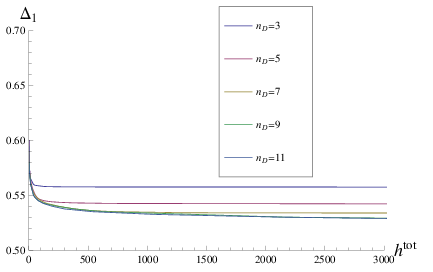
In figure 3 we have plotted the bound for various values of the order $n_{{{\mathcal{D}}}}$ of the differential operator. As expected, $\Delta_{1}$ is monotonically decreasing in $h^{\mathrm{tot}}$. We find that $\Delta_{1}$ converges very quickly in $n_{{{\mathcal{D}}}}$ for small Hodge numbers. The weakest bound is for vanishing Hodge numbers, for which we find $\Delta_{1}<0.60$. Note in particular that this means that the lowest lying state is always a non-BPS state.

For large Hodge numbers we have to go to higher and higher order to get a reliable result. This suggests that it is more efficient to perform a Taylor expansion around a point other than $\beta=1$. Using this one can in fact show that $\Delta_{1}\rightarrow\frac{1}{2}$ for $h^{\mathrm{tot}}\rightarrow\infty$. Note that $\frac{1}{2}=2\frac{c-c_{eff}}{24}$ corresponds to the $2\gamma$ we encountered in the bosonic case, where now $c=9$ and the effective central charge of the $N=2$ algebra is $c_{eff}=3$.

Let us briefly discuss the interpretation of this result. The bound we have found is uniform over the whole moduli space of a Calabi-Yau. As a toy model for this type of bound, take a free theory compactified on the torus. For large radius, the bound is satisfied by KK momentum modes. For very small radius, it is satisfied by the winding modes. Over the whole moduli space the gap becomes biggest at the self-dual point. Similarly, in general our bound $\Delta_{1}$ will be easily satsified by the eigenmodes of the Laplacian in the large volume limit. For small volumes, presumably it will again be easily satisfied by whatever corresponds to winding modes. We expect our bound to be most constraining in the highly stringy regime. One can conjecture the existence of a generalized self-dual point where our bound is actually saturated.

Note also that in principle this result makes a phenomenological prediction for type II compactifications, namely the existence of at least one stringy state below a certain threshold. This is a very weak bound since by the remarks above this state will have mass of the order of the string scale. Nonetheless this is one of very few $\alpha^{\prime}$ exact results that we are aware of. For a proper treatment one would have to perform the GSO projection, which will eliminate the tachyonic states with $h+\bar{h}<1$ that seem to appear in the spectrum so far.

Ultimately we would like to be able to rule out theories completely. One way we could have achieved that if the bound $\Delta_{1}$ had become negative for large enough $h^{\mathrm{tot}}$, which would have put an upper bound on the Hodge numbers of a CY 3-fold. This would give strong evidence in favor of the conjecture that there are only finitely many topological families of such manifolds [20].

Even though there is still some room for improvement on the bounds obtained from the partition function, it seems unlikely that this would be strong enough. We can show however that the number of states below $\Delta_{1}$ grows linearly in $h^{\mathrm{tot}}$ so that the spectrum becomes continuous as $h^{\mathrm{tot}}\rightarrow\infty$. We usually associate such a behavior with a decompactification limit, and by combining this result with other methods it may be possible to show inconsistency.

Ultimately what one should do is to probe deeper by combining modular invariance on the torus in an effective way with crossing symmetry on the sphere. This will presumably also allow to include other topological information such as the chiral ring of the CFT.

References

- [1] Maximo Banados, Claudio Teitelboim, and Jorge Zanelli, The Black hole in three-dimensional space-time, Phys.Rev.Lett. 69 (1992), 1849–1851.
- [2] Peter Bouwknegt, EXTENDED CONFORMAL ALGEBRAS, Phys.Lett. B207 (1988), 295.
- [3] Sheer El-Showk and Miguel F. Paulos, Bootstrapping Conformal Field Theories with the Extremal Functional Method, (2012).
- [4] Daniel Friedan and Christoph A. Keller, Constraints on 2d CFT partition functions, JHEP 1310 (2013), 180.
- [5] Daniel Friedan, Anatoly Konechny, and Cornelius Schmidt-Colinet, Lower bound on the entropy of boundaries and junctions in 1+1d quantum critical systems, Phys.Rev.Lett. 109 (2012), 140401.
- [6] by same author, Precise lower bound on Monster brane boundary entropy, JHEP 1307 (2013), 099.
- [7] Simeon Hellerman, A Universal Inequality for CFT and Quantum Gravity, JHEP 1108 (2011), 130.
- [8] Toshiya Kawai, Yasuhiko Yamada, and Sung-Kil Yang, Elliptic genera and N=2 superconformal field theory, Nucl.Phys. B414 (1994), 191–212.
- [9] Christoph A. Keller and Hirosi Ooguri, Modular Constraints on Calabi-Yau Compactifications, Commun.Math.Phys. 324 (2013), 107–127.
- [10] M. Fukuda K. Nakata M. Yamashita, K. Fujisawa and M. Nakata, A high-performance software package for semidefinite programs: SDPA 7, Research Report B-463, Dept. of Mathematical and Computing Science, Tokyo Institute of Technology, Tokyo, Japan, September 2010.
- [11] Alexander A. Migdal, Conformal invariance and bootstrap, Phys.Lett. B37 (1971), 386–388.
- [12] Gregory W. Moore and Nathan Seiberg, Classical and Quantum Conformal Field Theory, Commun.Math.Phys. 123 (1989), 177.
- [13] Satoru Odake, Extension of Superconformal Algebra and Calabi-yau Compactification, Mod.Phys.Lett. A4 (1989), 557.
- [14] by same author, C = 3- Conformal Algebra With Extended Supersymmetry, Mod.Phys.Lett. A5 (1990), 561.
- [15] Alexander M. Polyakov, Conformal symmetry of critical fluctuations, JETP Lett. 12 (1970), 381–383.
- [16] A.M. Polyakov, Nonhamiltonian approach to conformal quantum field theory, Zh.Eksp.Teor.Fiz. 66 (1974), 23–42.
- [17] Joshua D. Qualls and Alfred Shapere, Bounds on Operator Dimensions in 2D Conformal Field Theories, (2013).
- [18] Riccardo Rattazzi, Vyacheslav S. Rychkov, Erik Tonni, and Alessandro Vichi, Bounding scalar operator dimensions in 4D CFT, JHEP 0812 (2008), 031.
- [19] Edward Witten, Three-Dimensional Gravity Revisited, (2007).
- [20] S.-T. Yau, Review of geometry and analysis, Asian J. Math. 4 (2000), no. 1, 235–278, Kodaira’s issue.