End-to-End Delay Modeling for Mobile Ad Hoc Networks: A Quasi-Birth-and-Death Approach

Node mobility and channel models: As shown in Fig. 1 that we consider a unit torus MANET partitioned evenly into $m\times m$ cells [25, 9, 22]. In the concerned MANET, there are $n$ nodes moving around according to the i.i.d. mobility model [15, 23]. We consider the time slotted system, where each node randomly chooses one cell to move into at the beginning of every time slot and then stays in it for the whole time slot. We assume that a common bandwidth limited wireless channel is shared by all nodes for data transmissions. In each time slot, the data transmitted between any two nodes through the wireless channel is normalized to one packet.

Radio model: Each node employs the same radio power to transmit data through the common wireless channel. To enable the transmission region of a node (say $S$ in Fig. 1) to cover its own cell and also its $8$ neighbor cells (called coverage cells of the node hereafter), the corresponding radio range $r$ of the node should be set as $r=\sqrt{8}/m$. Based on the widely used protocol model [16, 20, 9, 22], data transmission from a transmitting node (transmitter) $i$ to a receiving node (receiver) $j$ can be conducted only if the Euclidean distance $d_{ij}$ between them is less than $r$ (i.e., $d_{ij}\leq r$), while the data can be successfully received by receiver $j$ only if $d_{kj}\geq(1+\Delta)\cdot r$ holds for any other concurrent transmitter $k$, here $k\neq i,j$, and $\Delta\geq 0$ is a specified guard-factor for interference prevention.

Traffic model: Similar to previous work [9], we consider the permutation traffic pattern in which each node acts as the source of a traffic flow and at the same time the destination of another traffic flow. Thus, there are in total $n$ distinct traffic flows in the MANET. Each source node exogenously generates packets for its destination according to an Bernoulli process with average rate $\lambda$ (packets/slot) [23].

For a fair channel access, we consider here a commonly used MAC protocol for transmission scheduling, based on the idea of equivalent-class (EC) [20, 9, 22]. An EC is defined as a set of cells as illustrated in Fig. 2, where any two cells in an EC are separated by a horizontal and vertical distance of some integer multiple of $\alpha$ cells ($1\leq\alpha\leq m$). Thus, we have in total $\alpha^{2}$ ECs in the MANET. Under the EC based MAC protocol (MAC-EC), these ECs are scheduled to be active alternatively as time evolves. The cells in an active EC are called active cells and nodes (if any) in an active cell contend fairly to access the common wireless channel.

To enable as many number of concurrent transmissions to be scheduled as possible while avoiding interference among these transmissions, the parameter $\alpha$ should be set appropriately. As illustrated in Fig 2 that for the transmission between a transmitter $S$ and its possible receiver $R$ to be successful, the distance between $R$ and another possible closest concurrent transmitter $W$, i.e., $(\alpha-2)/m$, should satisfy the following condition according to the protocol model [16]:

Notice also that $r=\sqrt{8}/m$ and $\alpha\leq m$, the parameter $\alpha$ should be determined as

where $\lceil x\rceil$ takes the least integer value greater than or equal to $x$.

Once a node, say $S$ in Fig. 2, succeeds in wireless channel contention and becomes a transmitter, it executes the popular two-hop relay (2HR) routing protocol defined in Algorithm 1 for packet delivery [11, 5]. With the 2HR routing, each exogenously generated packet at $S$ is first distributed out to relays through wireless broadcast [11, 24], and it is then delivered to its destination $D$ via these relays.

To facilitate the operation of the 2HR routing protocol, each node, say $S$, is equipped with three types of First In First Out (FIFO) queues: one source-queue, one broadcast-queue and $n-2$ parallel relay-queues (no relay-queue is needed for node $S$ itself and its destination node $D$).

Source-queue: Source-queue stores packets exogenously generated at $S$ and destined for $D$. These exogenous packets will be distributed out to relay nodes later in FIFS way.

Broadcast-queue: Broadcast-queue stores packets from source-queue that have already been distributed out by $S$ but have not been acknowledged yet by $D$ the reception of them.

Relay-queue: Each node other than $S$ and $D$ is assigned with a relay-queue in $S$ to store redundant copies of packets distributed out by the source of that node.

To ensure the in-order packet reception at $D$, similar to previous work [23] that $S$ labels every exogenously generated packet with a unique identification number $ID(S)$, which increases by $1$ every time a packet is generated; destination $D$ also maintains an acknowledgment number $ACK(D)$ indicating that $D$ is currently requesting the packet with $ID(S)=ACK(D)+1$ (i.e, the packets with $ID(S)\leq ACK(D)$ have already been received by $D$).

We focus on one specific traffic flow from source $S$ to destination $D$ in our analysis. Notice that once a packet is generated at $S$, it first experiences a queueing process in the source-queue of $S$ before being distributed out (served), and it then experiences a network delivery process after being distributed out into the network by $S$ and before being successfully received by $D$. Since $D$ requests packets in order according to $ACK(D)$, all packets distributed out by $S$ will be also delivered (served) in order. Thus, we can treat the network delivery process as a queueing process of one virtual network-queue. Notice also that the departure process of source-queue is just the arrival process of network-queue.

To fully depict the two queueing processes in both source-queue and network-queue, we define following probabilities for a time slot.

• •

  $p_{b}:$ probability that $S$ becomes transmitter and also selects to do packet-broadcast.

• •

  $p_{c}(j):$ probability that $j$ copies of a packet exist in the network (including the one in $S$) after the packet is distributed out by $S$ in the current time slot, $1\leq j\leq n-1$.

• •

  $p_{r}(j):$ probability that $D$ receives the packet it is currently requesting given that $j$ copies of the packet exist in the network, $1\leq j\leq n-1$.

• •

  $p_{0}(j):$ probability that $j$ copies of a packet exist in the network after $S$ becomes transmitter and selects to do packet-broadcast for this packet, given that $D$ is out of the coverage cells of $S$ and network-queue is empty, $1\leq j\leq n-1$.

• •

  $p_{0}(0):$ $p_{0}(0)=1-\sum_{j=1}^{n-1}p_{0}(j)$.

• •

  $p_{b}^{+}(j):$ probability that $S$ becomes transmitter, selects to do packet-broadcast and also successfully conducts packet-broadcast for one packet; at the same time, $D$ receives the packet it is requesting given that $j$ copies of that packet exist in the network, $1\leq j\leq n-1$.

• •

  $p_{b}^{-}(j):$ probability that $S$ becomes transmitter, selects to do packet-broadcast and also successfully conducts packet-broadcast for one packet; at the same time, $D$ does not receive the packet it is requesting given that $j$ copies of that packet exist in the network, $1\leq j\leq n-1$.

• •

  $p_{f}^{+}(j):$ probability that $S$ does not successfully conduct packet-broadcast for any packet; at the same time, $D$ receives the packet it is requesting given that $j$ copies of that packet exist in the network, $1\leq j\leq n-1$.

• •

  $p_{f}^{-}(j):$ probability that $S$ does not successfully conduct packet-broadcast for any packet; at the same time, $D$ does not receive the packet it is requesting given that $j$ copies of that packet exist in the network, $1\leq j\leq n-1$.

The following lemma reveals a nice property about the source-queue and network-queue, which will help us to evaluate the above probabilities in Lemma 2.

Lemma 1: For the considered MANET with MAC-EC protocol for transmission scheduling and 2HR-B protocol for packet delivery, the arrival process of network-queue is a Bernoulli process with probability $\lambda$ and it is independent of the state of source-queue.

Lemma 2:

where

Remark: The complex network dynamics of node mobility, interference, wireless channel and traffic contention are incorporated into the calculation of the above probabilities as shown in Appendix A. The network dynamics of packet distributing, packet queueing and delivering processes will be captured in the following QBD modeling process.

We use $L(t)\geq 0$ to denote the number of local packets distributed out from $S$ but not received yet by $D$ until time slot $t$, and use $J(t)$ to denote the number of copies of the packet $D$ is currently requesting at time slot $t$ in the network, $0\leq J(t)\leq n-1$. As time $t$ evolves, the queueing process of network-queue follows a two-dimensional QBD process [3, 21]

on state space

where $(0,0)$ corresponds to the empty network-queue state. $L(t)$ increases by $1$ if $S$ distributes out a packet from its source-queue while $D$ does not receive the packet it is requesting at slot $t$, $L(t)$ decreases by $1$ if $S$ does not distribute out a packet from its source-queue while $D$ receives the packet it is requesting at slot $t$, and $L(t)$ keeps unchanged, otherwise.

All states in (14) can be divided into the following subsets

where subset $N(0)$ is called level $0$ and subset $N(l)$ is called level $l$. It is notable that when network-queue is in some state of level $l$ ($l\geq 1$) at a time slot, the next state of one-step state transitions could only be some state in the same level $l$ or in its adjacent levels $l-1$ and $l+1$.

Based on the queueing process of network-queue and the definitions of probabilities in Lemma 2, the underlying QBD process of the network-queue has state transition diagram shown in Fig. 3. In Fig. 3, $p_{f}^{+}(\ast)p_{c}(j)$ denotes the probability of the transition from some state $(3,\ast)$ in level $3$ to the state $(2,j)$ in level $2$, where the asterisk ‘$\ast$’ means some eligible copy number in $\{1,2,\cdots,n-1\}$.

To facilitate our discussion, we classify the state transitions in Fig. 3 as intra-level transition (denoted by dotted arrows in Fig. 3) and inter-level transition (denoted by solid arrows in Fig. 3).

Intra-level Transition: There are two cases regarding the intra-level transitions, namely, the state transition inside level $0$ and the state transitions inside level $l$ ($l\geq 1$). For level $0$, it has only one state $(0,0)$, which could only transit to itself. For levels $l\geq 1$, they all follow the same intra-level transitions, i.e., a state $(l,j)$ in level $l$ could transit to any state (including itself) in the same level, $1\leq j\leq n-1$.

Inter-level Transition: There are also two cases regarding the inter-level transitions, namely, transitions between level $0$ and level $1$, and transitions between level $l$ and level $l+1$ ($l\geq 1$). The inter-level transitions between level $0$ and level $1$ are simply bi-transitions between state $(0,0)$ and any state $(1,j)$, $1\leq j\leq n-1$. For adjacent levels $l$ and $l+1$ ($l\geq 1$), they all follow the same inter-level transitions, i.e., a state $(l,j)$ in level $l$ could only transit to the corresponding state $(l+1,j)$ in level $l+1$, while a state $(l+1,j)$ in level $l+1$ could transit to any state in level $l$, $1\leq j\leq n-1$.

For networks of different size $n$, Fig. 4 shows both theoretical and simulation results on packet end-to-end delay under the settings of $m=16$, system load $\rho=0.6$ $(\rho=\lambda/\mu)$ and packet-broadcast probability $q=\{0.1,0.3,0.5\}$. Unless otherwise mentioned, simulation results are reported with small $95\%$ confidence intervals. The results in Fig. 4 show clearly that in a wide range of network scenarios considered here, theoretical results match very nicely with simulated ones, indicating that our QBD-based theoretical modeling is really efficient in capturing the expected packet end-to-end delay behavior of concerned MANETs. From Fig. 4 we can also see that as network size $n$ increases, packet end-to-end delay increases as well. This is because that in the concerned MANET with fixed unit area and fixed setting of $m=16$, as $n$ increases the contention for wireless channel access becomes more intensive, resulting in a lower packet delivery opportunity and thus a longer packet end-to-end delay.

For the setting of $n=150,m=16$ and $q=0.4$, Fig. 5 shows both the theoretical and simulation results on packet end-to-end delay when system load $\rho$ changes from $\rho=0.2$ to $\rho=0.9$. In addition to the i.i.d. mobility model considered in this paper, the corresponding simulation results for the random walk and random waypoint mobility models have also been included in Fig. 5 for comparison. Again, we can see from Fig. 5 that our theoretical delay model is very efficient. It is interesting to see from Fig. 5 that although our theoretical framework is developed under the i.i.d. mobility model, it can also nicely capture the general packet end-to-end delay behavior under more realistic random walk and random waypoint mobility models.

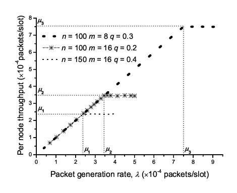
Another observation of Fig. 5 is that the packet end-to-end delay increases sharply as system load $\rho$ approaches $1.0$ (i.e., as packet generation rate $\lambda$ approaches per node throughput capacity $\mu$), which serves as an intuitive verification of our theoretical per node throughput capacity result. To further validate our theoretical model on throughput capacity, Fig. 6 provides the simulation results on the achievable per node throughput, i.e., the average rate of packet delivery to destination, when packet generation rate $\lambda$ increases gradually, where the results of three network scenarios with different throughput capacity $\{n=150,m=16,q=0.4,\mu_{1}=2.37\times 10^{-4}\}$, $\{n=100,m=16,q=0.2,\mu_{2}=3.46\times 10^{-4}\}$ and $\{n=100,m=8,q=0.3,\mu_{3}=7.52\times 10^{-4}\}$ are presented. We can see from Fig. 6 that for each network scenario there, the corresponding per node throughput first increases monotonously as $\lambda$ increases before $\lambda$ reaches the corresponding throughput capacity ($\mu_{1}$, $\mu_{2}$ and $\mu_{3}$), and then per node throughput remains a constant and does not increase anymore when packet generation rate $\lambda$ goes beyond the corresponding theoretical throughput capacity. Thus, our theoretical capacity model is also efficient in depicting the per node throughput capacity behavior of the considered MANET.

With the help of the QBD-based theoretical models, we explore how parameter $q$ of 2HR-B routing will affect the packet end-to-end delay $T_{e}$ and per node throughput capacity $\mu$ under given $m$, $n$ and $\rho$. The corresponding numerical results are summarized in Figs. 7 and 8.

We first examine the impact of $q$ on $T_{e}$. For network settings of $m=16$, $\rho=0.5$ and $n=\{80,300,500\}$, Fig. 7 shows that for a given network its delay $T_{e}$ always first decreases and then increases as $q$ increases. This phenomenon can be explained as follows. The end-to-end delay experienced by a packet consists of the time it spends in the source-queue and the time it spends in the network-queue. An increase in $q$ has two-fold effects on $T_{e}$: on one hand, it decreases the time a packet spends in the source-queue, because source $S$ has more chance to do packet-broadcast for packets in its source-queue, which makes the queue to be served more quickly; on the other hand, it increases the time a packet spends in the network-queue, because each relay has less chance to do packet-delivery to deliver a packet to destination $D$, which makes the network-queue to be served more slowly. Thus, $T_{e}$ decreases as $q$ increases when the first effect dominates the second one, while $T_{e}$ increases as $q$ increases when the second effect dominates the first one.

We next explore how parameter $q$ affects $\mu$. For network settings of $m=16$ and $n=\{80,300,500\}$, Fig. 8 shows that for a given network its capacity $\mu$ always first increases and then decreases as $q$ increases. Notice that $\mu$ is determined by the minimum of service rates of the source-queue and network-queue. When $q$ is small, $\mu$ is determined by the service rate of source-queue, which increases as $q$ increases. When $q$ is large, $\mu$ is determined by the service rate of network-queue, which decreases as $q$ increases. Another observation from Fig. 8 is that the capacity $\mu$ of $n=80$ is the largest among different $n$ there. This is because that for a MANET with fixed $m=16$, a larger number of nodes there will cause a more intensive wireless channel contention, which decrease opportunities of packet transmission and thus the per node throughput capacity.

References

- [1] C++ simulator for the 2HR-B MANETs. [Online]. Available: http://researchplatform.blogspot.jp/.
- [2] The network simulator ns-2. [Online]. Available: http://www.isi.edu/nsnam/ns/.
- [3] Attahiru Sule Alfa. (2010). Queueing Theory for Telecommunications: Discrete Time Modelling of a Single Node System. Springer.
- [4] Majed Alresaini, Maheswaran Sathiamoorthy, and Michael J. Neely. (2012). Backpressure with adaptive redundancy (bwar). In INFOCOM.
- [5] Eitan Altman, Tamer Basar, and Francesco De Pellegrini. (March 2011). Optimal control in two-hop relay routing. IEEE Transactions on Automatic Control, 56(3):670–675.
- [6] Jeffrey Andrews, Sanjay Shakkottai, Robert Heath, Nihar Jindal, Martin Haenggi, Randy Berry, Dongning Guo, Michael J. Neely, Steven Weber, Syed Jafar, and Aylin Yener. (December 2008). Rethinking information theory for mobile ad hoc networks. IEEE Communications Magazine, 46(12):94–101.
- [7] Dimitri P. Bertsekas and Robert G. Gallager. (1992). Data Networks. New Jersey: Prentice-Hall, Inc.
- [8] Florin Ciucu. (2011). Non-asymptotic capacity and delay analysis of mobile wireless networks. In SIGMETRICS.
- [9] Delia Ciullo, Valentina Martina, Michele Garetto, and Emilio Leonardi. (December 2011). Impact of correlated mobility on delay-throughput performance in mobile ad hoc networks. IEEE/ACM Transactions on Networking, 19(6):1745–1758.
- [10] Hans Daduna. (2001). Queueing Networks with Discrete Time Scale: Explicit Expressions for the Steady State Behavior of Discrete Time Stochastic Networks. Springer.
- [11] Renato M. de Moraes, Hamid R. Sadjadpour, and J.J. Garcia-Luna-Aceves. (June 2007). Taking full advantage of multiuser diversity in mobile ad hoc networks. IEEE Transactions on Communications, 55(6):1202 – 1211.
- [12] Oliver Hohlfeld Florin Ciucu and Pan Hui. (2010). Non-asymptotic throughput and delay distributions in multi-hop wireless networks. In Annual Allerton Conference on Communicaiton, Control, and Computing (Allerton).
- [13] Abbas El Gamal, James Mammen, Balaji Prabhakar, and Devavrat Shah. (June 2006). Optimal throughput-delay scaling in wireless networks-part i: The fluid model. IEEE Transactions on Information Theory, 52(6):2568–2592.
- [14] Andrea Goldsmith, Michelle Effros, Ralf Koetter, Muriel Médard, and Lizhong Zheng. (May 2011). Beyond shannon: the quest for fundamental performance limits of wireless ad hoc networks. IEEE Communications Magazine, 49(5):195–205.
- [15] Matthias Grossglauser and David N.C. Tse. (August 2002). Mobility increases the capacity of ad hoc wireless networks. IEEE/ACM Transactions on Networking, 10(4):477–486.
- [16] P. Gupta and P.R. Kumar. (March 2000). The capacity of wireless networks. IEEE Transactions on Information Theory, 46(2):388–404.
- [17] Ahmad Al Hanbali, Roland de Haan, Richard J. Boucherie, and Jan-Kees van Ommeren. (2008). A tandem queueing model for delay analysis in disconnected ad hoc networks. In Proceedings of the 15th international conference on Analytical and Stochastic Modeling Techniques and Applications (ASMTA), pages 189–205.
- [18] Lajos Hanzo II and Rahim Tafazolli. (2nd Quarter 2007). A survey of qos routing solutions for mobile ad hoc networks. IEEE Communications Surveys and Tutorials, 9(2):50–70.
- [19] Apoorva Jindal and Konstantinos Psounis. (February 2009). Contention-aware performance analysis of mobility-assisted routing. IEEE Transactions on Mobile Computing, 8(2):145–161.
- [20] Sanjeev R. Kulkarni and Pramod Viswanath. (June 2004). A deterministic approach to throughput scaling in wireless networks. IEEE Transactions on Information Theory, 50(6):1041–1049.
- [21] G. Latouche and V. Ramaswamy. (1999). Introduction to Matrix Analytic Methods in Stochastic Modeling. ASA-SIAM Series on Statistics and Applied Probability.
- [22] Pan Li, Yuguang Fang, Jie Li, and Xiaoxia Huang. (March 2012). Smooth trade-offs between throughput and delay in mobile ad hoc networks. IEEE Transactions on Mobile Computing, 11(3):427–438.
- [23] Michael J. Neely and Eytan Modiano. (June 2005). Capacity and delay tradeoffs for ad-hoc mobile networks. IEEE Transactions on Information Theory, 51(6):1917–1936.
- [24] Michael J. Neely and Rahul Urgaonkar. (July 2009). Optimal backpressure routing for wireless networks with multi-receiver diversity. Ad Hoc Networks, 7(5):862–881.
- [25] Gaurav Sharma, Ravi Mazumdar, and Ness B. Shroff. (October 2007). Delay and capacity trade-offs for mobile ad hoc networks: A global perspective. IEEE/ACM Transactions on Networking, 15(5):981–992.
- [26] Shan Zhou and Lei Ying. (2010). On delay constrained multicast capacity of large-scale mobile ad-hoc networks. In INFOCOM.