Multihop Backhaul Compression for the Uplink of Cloud Radio Access Networks

Seok-Hwan Park Osvaldo Simeone Onur Sahin Shlomo Shamai (Shitz) ^†^†thanks: S.-H. Park and O. Simeone are with the Center for Wireless Communications and Signal Processing Research (CWCSPR), ECE Department, New Jersey Institute of Technology (NJIT), Newark, NJ 07102, USA (email: {seok-hwan.park, osvaldo.simeone}@njit.edu). O. Sahin is with InterDigital Inc., Melville, New York, 11747, USA (email: Onur.Sahin@interdigital.com). S. Shamai (Shitz) is with the Department of Electrical Engineering, Technion, Haifa, 32000, Israel (email: sshlomo@ee.technion.ac.il).

Abstract

In cloud radio access networks (C-RANs), the baseband processing of the radio units (RUs) is migrated to remote control units (CUs). This is made possible by a network of backhaul links that connects RUs and CUs and that carries compressed baseband signals. While prior work has focused mostly on single-hop backhaul networks, this paper investigates efficient backhaul compression strategies for the uplink of C-RANs with a general multihop backhaul topology. A baseline multiplex-and-forward (MF) scheme is first studied in which each RU forwards the bit streams received from the connected RUs without any processing. It is observed that this strategy may cause significant performance degradation in the presence of a dense deployment of RUs with a well connected backhaul network. To obviate this problem, a scheme is proposed in which each RU decompresses the received bit streams and performs linear in-network processing of the decompressed signals. For both the MF and the decompress-process-and-recompress (DPR) backhaul schemes, the optimal design is addressed with the aim of maximizing the sum-rate under the backhaul capacity constraints. Recognizing the significant demands of the optimal solution of the DPR scheme in terms of channel state information (CSI) at the RUs, decentralized optimization algorithms are proposed under the assumption of limited CSI at the RUs. Numerical results are provided to compare the performance of the MF and DPR schemes, highlighting the potential advantage of in-network processing and the impact of CSI limitations.

Index Terms:

Index Terms— Cloud radio access network, multihop backhaul, mesh backhaul, compression, in-network processing.

I Introduction

Refer to caption — Figure 1: Illustration of the uplink of cloud radio access networks (C-RANs) with a multihop backhaul network (RU: Radio Unit, CU: Control Unit).

Cloud radio access networks (C-RANs) [1][2] prescribe the separation of localized and distributed radio units (RUs) from remote and centralized information processing nodes or control units (CUs). The centralization of information processing afforded by C-RANs potentially enables effective interference management at the geographical scale covered by the distributed RUs. The main roadblock to the realization of this potential hinges on the effective integration of the wireless interface provided by the RUs with the backhaul network [3][4].

With standard backhaul solutions based on the use of standard analog-to-digital conversion techniques in the uplink and standard digital-to-analog conversion techniques in the downlink [5], backhaul capacity limitations are known to impose a formidable bottleneck to the system performance (see, e.g., [4]). In order to alleviate the performance bottleneck identified above, recent efforts by industry and academia have targeted the design of more advanced backhaul compression schemes, which are based on point-to-point vector compression algorithms (see, e.g., [1] and also [6] for experimental result). Following information-theoretic insights, multiterminal, as opposed to point-to-point, backhaul compression techniques have been studied in [7]-[10] for the uplink and in [11] for the downlink.

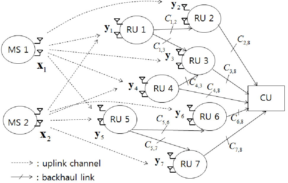
The research activity reviewed above assumes a single-hop, or star, backhaul topology in which each RU is directly connected to its managing CUs via a backhaul link. In this work, instead, we study a more general multihop backhaul topology in which each RU may communicate with the managing CU through a set of intermediate RUs as shown in Fig. 1. This backhaul topology is especially relevant for heterogeneous small-cell networks in which RUs of various sizes such as pico/femto or macro base stations are connected by a mesh backhaul network [12] (see also the standard [5]).

Reference [13] provides a simulation-based study of the performance of uplink C-RANs over multihop networks under the assumption that each RU is able to evaluate the log-likelihood ratios of the transmitted bits of the connected mobile stations (MSs). In-network processing of the log-likelihood ratios is proposed to enhance the effectiveness of the use of the backhaul network. In this paper, we instead focus on RUs that directly compress the received baseband signal without performing any demodulation, following the standard set-up for C-RAN (see, e.g., [2][5]). Reference [14] studies the related problem of optimizing linear in-network processing operations in multihop network within the context of estimation (and not reliable digital communication). The advantages of in-network processing were also investigated in [15] for function computation in distributed sensor networks. We finally point to related research activity on the performance of multihop Gaussian relay networks with compress-and-forward strategies, single-antenna nodes and fixed compression strategies, such as [16]-[18] (see also [19][20]).

The paper organization and main contributions are as follows.

•

In Sec. II, we present the system model and describe the general structure of backhaul routing strategies;
•

We investigate the Multiplex-and-Forward (MF) scheme in Sec. III, whereby each RU forwards the bit streams received from the connected RUs without any processing;
•

It is observed that this strategy may incur significant performance degradation when the RUs have a sufficiently large number of incoming backhaul links. In fact, in this case, the bit rate obtained by multiplexing the signals received from the connected RUs is large and the backhaul capacity constraints may impose a critical performance bottleneck;
•

We propose and investigate the Decompress-Process-and-Recompress (DPR) scheme that performs linear in-network processing of the compressed baseband signals. The proposed DPR strategy performs the joint optimization of the linear processing matrices and the compression strategies by assuming that each RU has full channel state information (CSI);
•

Since the full CSI assumption at each RU may not be practical when the number of RUs grows large, in Sec. V, we propose decentralized DPR strategies whereby each RU computes its linear processing and compression strategies using only local CSI;
•

We discuss an extension of the DPR scheme to the case in which there are multiple CUs connected to each other on the backhaul network in Sec. IV-C;
•

Finally, in Sec. VI, we provide extensive numerical results to assess the performance of the considered schemes.

We conclude the paper in Sec. VII.

Notation: We adopt standard information-theoretic definitions for the mutual information $I(X;Y)$ between the random variables $X$ and $Y$ , conditional mutual information $I(X;Y|Z)$ between $X$ and $Y$ conditioned on random variable $Z$ [21]. All logarithms are in base two unless specified. The circularly symmetric complex Gaussian distribution with mean ${\mu}$ and covariance matrix $\mathbf{R}$ is denoted by $\mathcal{CN}(\mbox{\boldmath${\mu}$},\mathbb{R})$ . The set of all $M\times N$ complex matrices is denoted by $\mathbb{C}^{M\times N}$ , and $\mathbb{E}[\cdot]$ represents the expectation operator. We use the notation $\mathbf{X}\succeq\mathbf{0}$ to indicate that the matrix $\mathbf{X}$ is positive semidefinite. The operation $(\cdot)^{\dagger}$ denotes Hermitian transpose of a matrix or vector, and notation $\mathbf{\Sigma}_{\mathbf{x}}$ is used for the correlation matrix of random vector $\mathbf{x}$ , i.e., $\mathbf{\Sigma}_{\mathbf{x}}=\mathbb{E}[\mathbf{x}\mathbf{x}^{\dagger}]$ ; $\mathbf{\Sigma}_{\mathbf{x},\mathbf{y}}$ represents the cross-correlation matrix $\mathbf{\Sigma}_{\mathbf{x},\mathbf{y}}=\mathbb{E}[\mathbf{x}\mathbf{y}^{\dagger}]$ ; $\mathbf{\Sigma}_{\mathbf{x}|\mathbf{y}}$ is used for the conditional correlation matrix, i.e., $\mathbf{\Sigma}_{\mathbf{x}|\mathbf{y}}=\mathbb{E}[\mathbf{x}\mathbf{x}^{\dagger}|\mathbf{y}]$ , and computed as $\mathbf{\Sigma}_{\mathbf{x}|\mathbf{y}}=\mathbf{\Sigma}_{\mathbf{x}}-\mathbf{\Sigma}_{\mathbf{x},\mathbf{y}}\mathbf{\Sigma}_{\mathbf{y}}^{-1}\mathbf{\Sigma}_{\mathbf{x},\mathbf{y}}^{\dagger}$ . Given a sequence of matrices $\mathbf{X}_{1},\ldots,\mathbf{X}_{m}$ , we define the notation $[\mathbf{X}_{1};\ldots;\mathbf{X}_{m}]=[\mathbf{X}_{1}^{\dagger},\ldots,\mathbf{X}_{m}^{\dagger}]^{\dagger}$ and the matrix $\mathbf{X}_{\mathcal{S}}$ for a subset $\mathcal{S}\subseteq\{1,\ldots,m\}$ as the matrix including, in ascending order, the matrices $\mathbf{X}_{i}$ with $i\in\mathcal{S}$ .

II System Model

We consider the uplink of a C-RAN in which $N_{M}$ MSs transmit information over a shared wireless medium to $N_{R}$ RUs as depicted in Fig. 1. The RUs are connected among themselves and to the CUs that perform decoding of the MSs’ information via a multihop network of backhaul links. We define as $\mathcal{N}_{M}=\{1,\ldots,N_{M}\}$ and $\mathcal{N}_{R}=\{1,\ldots,N_{R}\}$ the sets of MSs and RUs, respectively. MS $k$ and RU $i$ are equipped with $n_{M,k}$ and $n_{R,i}$ antennas, respectively, for $k\in\mathcal{N}_{M}$ and $i\in\mathcal{N}_{R}$ . The total number of MSs’ antennas is denoted as $n_{M}=\sum_{k\in\mathcal{N}_{M}}n_{M,k}$ . Fig. 1 is an example with $N_{R}=7$ RUs, $N_{M}=2$ MSs, a single CU and $n_{M,k}=n_{R,i}=2$ antennas at each terminal for $k\in\mathcal{N}_{M}$ and $i\in\mathcal{N}_{R}$ .

II-A Channel Model

Here we discuss the wireless uplink channel between MSs and RUs and the multihop backhaul network connecting RUs and the CU. Specifically, in most of the paper, we consider the case with a single CU, while the more general scenario with multiple CUs is briefly treated in Sec. IV-C (see Fig. 5 for an illustration).

Uplink: On the uplink channel, the signal $\mathbf{y}_{i}\in\mathbb{C}^{n_{R,i}\times 1}$ received by RU $i$ at a given time is given by

\mathbf{y}_{i}=\mathbf{H}_{i}\mathbf{x}+\mathbf{z}_{i},

(1)

where $\mathbf{x}=[\mathbf{x}_{1};\mathbf{x}_{2};\ldots;\mathbf{x}_{N_{M}}]$ is the signal transmitted by all MSs with $\mathbf{x}_{k}\in\mathbb{C}^{n_{M,k}\times 1}$ denoting the signal transmitted by MS $k$ ; $\mathbf{H}_{i}\in\mathbb{C}^{n_{R,i}\times n_{M}}$ is the flat-fading channel response matrix from all MSs toward RU $i$ ; and $\mathbf{z}_{i}\in\mathbb{C}^{n_{R,i}\times 1}$ is the additive noise at RU $i$ , which is distributed as $\mathbf{z}_{i}\sim\mathcal{CN}(\mathbf{0},\mathbf{I})$ . The signal $\mathbf{x}$ is distributed as $\mathbf{x}\sim\mathcal{CN}(\mathbf{0},\mathbf{\Sigma}_{\mathbf{x}})$ with covariance matrix $\mathbf{\Sigma}_{\mathbf{x}}=\mathrm{diag}(\mathbf{\Sigma}_{\mathbf{x}_{1}},\ldots,\mathbf{\Sigma}_{\mathbf{x}_{N_{M}}})$ . Note that the signals $\mathbf{x}_{k}$ are independent for $k\in\mathcal{N}_{M}$ , since the MSs are not able to cooperate. As a result, the signal $\mathbf{y}=[\mathbf{y}_{1};\mathbf{y}_{2};\ldots;\mathbf{y}_{N_{R}}]$ received by all RUs is distributed as $\mathbf{y}\sim\mathcal{CN}(\mathbf{0},\mathbf{\Sigma}_{\mathbf{y}})$ with $\mathbf{\Sigma}_{\mathbf{y}}=\mathbf{H}\mathbf{\Sigma}_{\mathbf{x}}\mathbf{H}^{\dagger}+\mathbf{I}$ and $\mathbf{H}=[\mathbf{H}_{1};\mathbf{H}_{2};\ldots;\mathbf{H}_{N_{R}}]$ .

Backhaul network: In order to model the backhaul multihop network connecting the RUs and the CU, we define a capacitated directed acyclic graph $\mathcal{G}=(\mathcal{V},\mathcal{E})$ (see, e.g., [22]). Accordingly, the set of vertex nodes of the directed acyclic graph is $\mathcal{V}=\mathcal{N}_{R}\cup\{N_{R}+1\}$ , where the node $i$ represents the $i$ th RU for $i\in\mathcal{N}_{R}$ and the last node $N_{R}+1$ stands for the CU. Also, the set $\mathcal{E}\subseteq\mathcal{V}\times\mathcal{V}$ contains the edges, where an edge $e=(i,j)$ represents the backhaul link of capacity $C_{i,j}$ bits/s/Hz connecting node $i$ to node $j$ . The capacity $C_{i,j}$ is normalized by the bandwidth used on the uplink wireless channel (as in, e.g., [23]). Note that this enables the capacity $C_{i,j}$ to be equivalently measured in bits per channel use of the uplink. The head and tail of edge $e=(i,j)$ with respect to the direction $i\rightarrow j$ are denoted by $\mathrm{head}(e)=j$ and $\mathrm{tail}(e)=i$ , respectively.

Remark 1.

In the given system model, all the RUs generally serve the double purpose of radio receivers on the uplink and of intermediate hops between “upstream” RUs and the CU on the backhaul network. In practice, some nodes may not operate as radio receivers but only as intermediate nodes in the backhaul network. This situation is captured by the model by setting the channel matrix $\mathbf{H}_{i}$ in (1) to have all-zero entries for all such nodes. In the following, we hence refer to all nodes that belong to the backhaul network as RUs with the understanding that some of them may only serve as relays.

II-B Backhaul Routing

As discussed in Sec. I, we will consider different strategies for the transmission of the RUs’ baseband received signals to the CU on the backhaul network. For all schemes, routing from the RUs to the CU can be described as detailed in this subsection following similar treatments in [14][24]. To this end, we fix an ordered partition of the set $\mathcal{V}$ , which includes the RUs and the CU, into layers $\mathcal{V}_{1},\ldots,\mathcal{V}_{L}$ , so that $\mathcal{V}=\bigcup_{l=1}^{L}\mathcal{V}_{l}$ and $\mathcal{V}_{m}\bigcap\mathcal{V}_{l}=\textrm{�}$ for $m\neq l$ with $N_{R}+1\in\mathcal{V}_{L}$ . Each partition gives rise to a specific routing schedule, as discussed next.

Given a partition $\mathcal{V}_{1},\ldots,\mathcal{V}_{L}$ , we consider as active, and hence available for routing, only the edges, i.e., the backhaul links, that connect nodes belonging to successive layers. More precisely, we define the set $\mathcal{E}_{\mathrm{act}}$ of the active edges as

\mathcal{E}_{\mathrm{act}}=\left\{e\in\mathcal{E}|\mathrm{tail}(e)\in\mathcal{V}_{l}\,\mathrm{and}\,\mathrm{head}(e)\in\mathcal{V}_{k}\,\,\mathrm{with}\,\,l<k\right\}.

(2)

Moreover, we define as $\Gamma_{I}(i)=\{e_{1}^{i},\ldots,e_{|\Gamma_{I}(i)|}^{i}\}$ and $\Gamma_{O}(i)$ the sets of active edges that end or originate at node $i$ , respectively. In other words, we have $\Gamma_{I}(i)=\{e\in\mathcal{E}_{\mathrm{act}}|\mathrm{head}(e)=i\}$ and $\Gamma_{O}(i)=\{e\in\mathcal{E}_{\mathrm{act}}|\mathrm{tail}(e)=i\}$ . The set of nodes that do not have any incoming active edge is denoted by $\mathcal{S}=\{i\in\mathcal{V}|\Gamma_{I}(i)=\textrm{�}\}$ .

A given ordered partition $\mathcal{V}_{1},\ldots,\mathcal{V}_{L}$ defines a routing strategy as follows. Each node $i$ in the first layer, i.e., with $i\in\mathcal{V}_{1}$ , transmits on the active backhaul links $e\in\Gamma_{O}(i)$ to the nodes in the next layers $\mathcal{V}_{l}$ , $l>1$ . The nodes in the second layer $\mathcal{V}_{2}$ wait until all the nodes in the same layer receive from the connected nodes in $\mathcal{V}_{1}$ and then transmit on the active backhaul links to the nodes in the next layers $\mathcal{V}_{l}$ with $l>2$ . In general, the nodes in each layer $\mathcal{V}_{l}$ wait for all the nodes in the same layer to receive from the previous layers $\mathcal{V}_{1},\ldots,\mathcal{V}_{l-1}$ and then transmit on the active backhaul links to the nodes in the next layers $\mathcal{V}_{l+1},\ldots,\mathcal{V}_{L}$ .

Fig. 2 presents two different routing examples for a backhaul network with $N_{R}=4$ RUs. For routing strategy 1 in the figure, the partition is defined as $\mathcal{V}_{1}=\{1,2\},\mathcal{V}_{2}=\{3,4\},\mathcal{V}_{3}=\{5\}$ , and, as a result, all edges in $\mathcal{E}$ are active, i.e., $\mathcal{E}_{\mathrm{act}}=\mathcal{E}$ . Instead, with routing strategy 2, we have the partition $\mathcal{V}_{1}=\{1,2,3,4\},\mathcal{V}_{2}=\{5\}$ and thus only edges $(1,5)$ , $(3,5)$ and $(4,5)$ are active, i.e., $\mathcal{E}_{\mathrm{act}}=\{(1,5),(3,5),(4,5)\}$ . Note that, with this strategy, node $2$ does not contribute to the operation of the network.

Remark 2.

Using classical results in graph theory, it follows that, for a given directed acyclic graph $\mathcal{G}=(\mathcal{V},\mathcal{E})$ , there always exists a partition $\mathcal{V}_{1},\ldots,\mathcal{V}_{L}$ that leads to activate all edges, i.e., to have $\mathcal{E}_{\mathrm{act}}=\mathcal{E}$ (see, e.g., [25, Sec. 2.1]).

We now discuss how the choice of the routing strategy and the the tolerated delay for communication from the RUs to the CU affect the use of the capacity of each backhaul link. To start, for a given set $\mathcal{E}_{\mathrm{act}}$ of active edges, we define as $D_{i}$ the number of edges in the longest path connecting the node $i$ to the CU $N_{R}+1$ . For example, in Fig. 2, we have $(D_{1},D_{2},D_{3},D_{4})=(2,2,1,1)$ and $(D_{1},D_{3},D_{4})=(1,1,1)$ for routing strategies 1 and 2, respectively. Then, we define the depth $D$ of a routing strategy defined by the partition $\mathcal{V}_{1},\ldots,\mathcal{V}_{L}$ as $D=\max_{i\in\mathcal{S}}D_{i}$ .

Define as $T$ the maximum delay allowed for transmission of the received baseband signals from the RUs to the CU. We normalize $T$ by the duration of the transmission on the uplink, so that $T=1$ means that the delay allowed for transmission on the backhaul network equals the duration of the uplink transmission. Assuming for simplicity that each active backhaul link is used for the same amount of time, we then obtain that each active edge is used only for a period equal to $T/D$ uplink slots. Therefore, the effective backhaul capacity $\tilde{C}_{e}$ used on an edge $e\in\mathcal{E}_{\mathrm{act}}$ , i.e., the number of bits per channel use of the uplink that are transmitted on a given active edge $e$ , equals $\tilde{C}_{e}=C_{e}\cdot T/D$ . For instance, if $T=D$ , and hence a delay equal to the depth of the routing strategy is tolerated, then we have $\tilde{C}_{e}=C_{e}$ . In this case, in fact, each backhaul link can be activated for the time duration equal to the wireless uplink transmission block.

III Multiplex-and-Forward

In this section, we present a reference scheme, which we refer to as Multiplex-and-Forward (MF). In this scheme, as illustrated in Fig. 3, each RU $i$ performs compression of its received baseband signal $\mathbf{y}_{i}$ using a given quantization codebook and then simply multiplexes the bit streams received from the previous layers and its compressed signal without any further processing. Specifically, each RU $i$ transmits on each of its outgoing backhaul links in $\Gamma_{O}(i)$ the bits describing the compressed baseband signal $\hat{\mathbf{y}}_{i}$ within the used quantization codebook along with the bit streams received from the previous layers. With this scheme, we hence only need to optimize the compression strategy used to produce $\hat{\mathbf{y}}_{i}$ and the allocation of the backhaul capacity among the received bit streams and the compressed signal $\hat{\mathbf{y}}_{i}$ .

In order to formulate this problem, we define as $f_{e}^{i}\geq 0$ the rate (in bits per channel use of the uplink) used to convey the compressed signal of RU $i$ on edge $e$ for $(i,e)\in\mathcal{N}_{R}\times\mathcal{E}_{\mathrm{act}}$ . By the definition of the routing scheme, we have the following constraints on the flow variables $f_{e}^{i}$

$\displaystyle f_{e}^{i}\geq$	$\displaystyle R_{i},\,\,\mathrm{for}\,\,i\in\mathcal{N}_{R}\,\,\mathrm{and}\,\,e\in\Gamma_{O}(i),$	(3)
$\displaystyle\sum_{e\in\Gamma_{I}(N_{R}+1)}f_{e}^{i}\geq$	$\displaystyle R_{i},\,\,\mathrm{for}\,\,i\in\mathcal{N}_{R},$	(4)
$\displaystyle\sum_{i\in\mathcal{N}_{R}}f_{e}^{i}\leq$	$\displaystyle\tilde{C}_{e},\,\,\mathrm{for}\,\,e\in\mathcal{E}_{\mathrm{act}},$	(5)
$\displaystyle\mathrm{and}\,\,\sum_{e\in\Gamma_{I}(j)}f_{e}^{i}\geq$	$\displaystyle\sum_{e\in\Gamma_{O}(j)}f_{e}^{i},\,\,\mathrm{for}\,\,(j,i)\in\mathcal{N}_{R}\times\mathcal{N}_{R},$	(6)

where $R_{i}$ represents the rate at which RU $i$ compresses its baseband signal $\mathbf{y}_{i}$ . This information must be sent on all the outgoing links $\Gamma_{O}(i)$ as per (3). The condition (4) guarantees that the CU $N_{R}+1$ receives sufficient information to be able to decompress, and the constraints (5) impose that the sum of the capacities $\{f_{e}^{i}\}_{i\in\mathcal{N}_{R}}$ passing through an edge $e$ does not exceed the effective capacity $\tilde{C}_{e}$ . The last condition (6) represents the flow conservation rule at each RU $j\in\mathcal{N}_{R}$ .

In order to describe the relationship between the rate $R_{i}$ and the fidelity of the compressed signal $\hat{\mathbf{y}}_{i}$ , we use standard rate distortion theoretic arguments (e.g., [21, Ch. 3]). Specifically, as in, e.g., [8][26][27], we assume a Gaussian quantization noise (without claim of optimality), so that the signal $\mathbf{\hat{\boldsymbol{\mathrm{y}}}}_{i}$ is given by¹¹ 1 As discussed in [8], the model (7) is as general as the model $\mathbf{\hat{\boldsymbol{\mathrm{y}}}}_{i}=\mathbf{L}_{i}\mathbf{y}_{i}+\mathbf{q}_{i}$ that contains a linear processing $\mathbf{L}_{i}$ prior to compression.

\mathbf{\hat{\boldsymbol{\mathrm{y}}}}_{i}=\mathbf{y}_{i}+\mathbf{q}_{i}.

(7)

In (7), $\mathbf{q}_{i}$ represents the quantization noise, which is distributed as $\mathcal{CN}(\mathbf{0},\mathbf{\Omega}_{i})$ and is independent of $\mathbf{y}_{i}$ . From rate-distortion theory, the compressed signal $\mathbf{\hat{\boldsymbol{\mathrm{y}}}}_{i}$ in (7) can be obtained at the output of the compressor if the rate $R_{i}$ satisfies the inequality [21, Ch. 3]

	$\displaystyle g_{i}^{\mathrm{MF}}\left(\{\mathbf{\Omega}_{i}\}_{i\in\mathcal{M}}\right)\triangleq$	$\displaystyle I\left(\mathbf{y}_{i};\mathbf{\hat{\boldsymbol{\mathrm{y}}}}_{i}\right)$		(8)
	$\displaystyle=$	$\displaystyle\log\det\left(\mathbf{\Omega}_{i}+\mathbf{\Sigma}_{\mathbf{y}_{i}}\right)-\log\det\left(\mathbf{\Omega}_{i}\right)\leq R_{i}.$

Based on the discussion above, as long as the constraints (3)-(6) and (8) are satisfied, the CU is able to recover the signals $\hat{\mathbf{y}}_{i}$ , $i\in\mathcal{N}_{R}$ , and an achievable sum-rate $R_{\mathrm{sum}}$ between the MSs and the CU is given as

	$\displaystyle R_{\mathrm{sum}}=$	$\displaystyle I\left(\mathbf{x};\{\mathbf{\hat{\boldsymbol{\mathrm{y}}}}_{i}\}_{i\in\mathcal{N}_{R}}\right)=f^{\mathrm{MF}}\left(\{\mathbf{\Omega}_{i}\}_{i\in\mathcal{N}_{R}}\right)$		(9)
	$\displaystyle\triangleq$	$\displaystyle\log\det\left(\mathbf{H}\mathbf{\Sigma}_{\mathbf{x}}\mathbf{H}^{\dagger}+\mathbf{I}+\mathbf{\Omega}\right)-\log\det\left(\mathbf{I}+\mathbf{\Omega}\right),$

with the definition $\mathbf{\Omega}=\mathrm{diag}(\mathbf{\Omega}_{1},\ldots,\mathbf{\Omega}_{N_{R}})$ .

III-A Problem Definition and Optimization

For a given routing strategy defined by the partition $\mathcal{V}_{1},\ldots,\mathcal{V}_{L}$ , we aim at optimizing the compression strategies $\{\mathbf{\Omega}_{i}\}_{i\in\mathcal{N}_{R}}$ and the flow variables $\{f_{e}^{i}\}_{i\in\mathcal{N}_{R},e\in\mathcal{E}_{\mathrm{act}}}$ with the goal of maximizing the sum-rate $R_{\mathrm{sum}}$ in (9) subject to the constraints (3)-(6) and (8). This problem is stated as


$\displaystyle\underset{\begin{array}[]{c}\{\mathbf{\Omega}_{i}\succeq\mathbf{0},R_{i}\geq 0\}_{i\in\mathcal{N}_{R}},\\ \{f_{e}^{i}\geq 0\}_{i\in\mathcal{N}_{R},e\in\mathcal{E}_{\mathrm{act}}}\end{array}}{\mathrm{maximize}}$	$\displaystyle f^{\mathrm{MF}}\left(\{\mathbf{\Omega}_{i}\}_{i\in\mathcal{N}_{R}}\right)$
$\displaystyle\mathrm{s.t.}\,\,\,\,\,\,$	$\displaystyle g_{i}^{\mathrm{MF}}\left(\{\mathbf{\Omega}_{i}\}_{i\in\mathcal{N}_{R}}\right)\leq R_{i},\,\,\mathrm{for}\,\,i\in\mathcal{N}_{R},$	(10c)
	$\displaystyle(\ref{eq:compression-rate-outgoing})-(\ref{eq:flow-conversion-rule}).$	(10d)

We note that the optimization (10) requires full CSI.

The problem (10) with respect to the variables $\{\mathbf{\Omega}_{i}\}_{i\in\mathcal{N}_{R}}$ and $\{f_{e}^{i}\geq 0\}_{i\in\mathcal{N}_{R},e\in\mathcal{E}_{\mathrm{act}}}$ is a difference-of-convex problem, which is a subclass of non-convex problems with desirable properties [28]. The problem is a difference-of-convex problem because the functions $f^{\mathrm{MF}}(\{\mathbf{\Omega}_{i}\}_{i\in\mathcal{N}_{R}})$ and $g_{i}^{\mathrm{MF}}(\{\mathbf{\Omega}_{i}\}_{i\in\mathcal{N}_{R}})$ can be written as the difference of convex functions and all other constraints in (10d) are linear. For difference-of-convex problems, the Majorization and Minimization (MM) algorithm provides an iterative procedure that is known to converge to a stationary point of the problem (see, e.g., [28]). The detailed algorithm is described in Algorithm 1, where we have defined for brevity the functions $\tilde{f}^{\mathrm{MF}}(\{\mathbf{\Omega}_{i}^{(t+1)},\mathbf{\Omega}_{i}^{(t)}\}_{i\in\mathcal{N}_{R}})$ and $\tilde{g}_{i}^{\mathrm{MF}}(\{\mathbf{\Omega}_{i}^{(t+1)},\mathbf{\Omega}_{i}^{(t)}\}_{i\in\mathcal{N}_{R}})$ as

$\displaystyle\tilde{f}^{\mathrm{MF}}\left(\{\mathbf{\Omega}_{i}^{(t+1)},\mathbf{\Omega}_{i}^{(t)}\}_{i\in\mathcal{N}_{R}}\right)\triangleq$	$\displaystyle\log\det\left(\mathbf{H}\mathbf{\Sigma}_{\mathbf{x}}\mathbf{H}^{\dagger}+\mathbf{I}+\mathbf{\Omega}^{(t+1)}\right)$	(11)
$\displaystyle-$	$\displaystyle\varphi(\mathbf{I}+\mathbf{\Omega}^{(t+1)},\mathbf{I}+\mathbf{\Omega}^{(t)})$
$\displaystyle\mathrm{and}\,\,\tilde{g}_{i}^{\mathrm{MF}}\left(\{\mathbf{\Omega}_{i}^{(t+1)},\mathbf{\Omega}_{i}^{(t)}\}_{i\in\mathcal{N}_{R}}\right)\triangleq$	$\displaystyle\varphi(\mathbf{\Omega}_{i}^{(t+1)}+\mathbf{\Sigma}_{\mathbf{y}_{i}},\mathbf{\Omega}_{i}^{(t)}+\mathbf{\Sigma}_{\mathbf{y}_{i}})-\log\det\left(\mathbf{\Omega}_{i}^{(t+1)}\right),$	(12)

with the function $\varphi(\mathbf{X},\mathbf{Y})$ given as

\varphi(\mathbf{X},\mathbf{Y})\triangleq\log\det\left(\mathbf{Y}\right)+\frac{1}{\ln 2}\mathrm{tr}\left(\mathbf{Y}^{-1}\left(\mathbf{X}-\mathbf{Y}\right)\right).

(13)

Algorithm 1 MF: MM Algorithm for problem (10)

1. Initialize the matrices $\{\mathbf{\Omega}_{i}^{(1)}\}_{i\in\mathcal{N}_{R}}$ to arbitrary feasible positive semidefinite matrices for problem (10) and set $t=1$ .

2. Update the matrices $\{\mathbf{\Omega}_{i}^{(t+1)}\}_{i\in\mathcal{N}_{R}}$ and variables $\{f_{e}^{i}\geq 0\}_{i\in\mathcal{N}_{R},e\in\mathcal{E}_{\mathrm{act}}}$ as a solution of the following convex problem:

	$\displaystyle\underset{\begin{array}[]{c}\{\mathbf{\Omega}_{i}^{(t+1)}\succeq\mathbf{0},R_{i}\geq 0\}_{i\in\mathcal{N}_{R}},\\ \{f_{e}^{i}\geq 0\}_{i\in\mathcal{N}_{R},e\in\mathcal{E}_{\mathrm{act}}}\end{array}}{\mathrm{maximize}}$	$\displaystyle\tilde{f}^{\mathrm{MF}}\left(\{\mathbf{\Omega}_{i}^{(t+1)},\mathbf{\Omega}_{i}^{(t)}\}_{i\in\mathcal{N}_{R}}\right)$
	$\displaystyle\mathrm{s.t.}\,\,\,\,\,\,\,\,\,$	$\displaystyle\tilde{g}_{i}^{\mathrm{MF}}\left(\{\mathbf{\Omega}_{i}^{(t+1)},\mathbf{\Omega}_{i}^{(t)}\}_{i\in\mathcal{N}_{R}}\right)\leq R_{i},\,\,\mathrm{for}\,\,i\in\mathcal{N}_{R},$
		$\displaystyle(\ref{eq:compression-rate-outgoing})-(\ref{eq:flow-conversion-rule}).$

3. Stop if a convergence criterion is satisfied. Otherwise, set $t\leftarrow t+1$ and go back to Step 2.

IV Decompress-Process-and-Recompress

The MF backhaul strategy studied in the previous section may incur a significant performance degradation when the RUs have a sufficiently large number of incoming edges. In fact, in this case, the bit rate obtained by multiplexing the signals received from the RUs in the previous layers is large and the backhaul capacity constraints may impose a critical performance bottleneck. In this section, we introduce a scheme that attempts to solve this problem via decompression at each RU and linear in-network processing of the decompressed signals and of the locally received signal. The key idea is that the processing step can reduce redundancy by properly combining the available (compressed) received signals. On the flip side, the processed signals need to be recompressed before they can be sent on the backhaul links. As discussed in [29] in the context of a cascade source coding problem, this recompression step introduces further distortion. The effect of this distortion must thus be counterbalanced by the advantages of in-network processing in order to make the strategy preferable to MF.

We now detail the DPR scheme and analyze its performance. As shown in Fig. 4, each RU $i$ first decompresses the signals $\mathbf{u}_{e^{\prime}}$ received on its incoming edges $e^{\prime}\in\Gamma_{I}(i)$ . Then, for each outgoing edge $e\in\Gamma_{O}(i)$ , it processes the vector $\mathbf{r}_{i}$ that includes the decompressed signals $\mathbf{u}_{e^{\prime}}$ for all edges $e^{\prime}\in\Gamma_{I}(i)$ and the received baseband signal $\mathbf{y}_{i}$ , namely

\mathbf{r}_{i}=[\mathbf{y}_{i};\mathbf{u}_{e_{1}^{i}};\cdots;\mathbf{u}_{e_{\left|\Gamma_{I}(i)\right|}^{i}}],

(16)

via a linear processing matrix $\mathbf{L}_{e}$ . This produces a processed signal $\mathbf{L}_{e}\mathbf{r}_{i}$ for all outgoing edges $e\in\Gamma_{O}(i)$ . We assume here that matrix $\mathbf{L}_{e}$ is square and study the issue of dimensionality reduction via the use of “wide” matrices $\mathbf{L}_{e}$ in Sec. IV-B. Note that the matrix $\mathbf{L}_{e}$ can be written as

\mathbf{L}_{e}=[\mathbf{L}_{e}^{\mathrm{rx}}\,\mathbf{L}_{e}^{e_{1}^{i}}\,\cdots\,\mathbf{L}_{e}^{e_{\left|\Gamma_{I}(i)\right|}^{i}}],

(17)

where, by (16), the matrices $\mathbf{L}_{e}^{\mathrm{rx}}\in\mathbb{C}^{d_{e}\times n_{R,i}}$ and $\mathbf{L}_{e}^{e_{j}^{i}}\in\mathbb{C}^{d_{e}\times d_{e_{j}^{i}}}$ multiply the signals $\mathbf{y}_{i}$ and $\mathbf{u}_{e_{j}^{i}}$ , respectively, for $j\in\{1,\ldots,\left|\Gamma_{I}(i)\right|\}$ . Finally, RU $i$ compresses the processed signal $\mathbf{L}_{e}\mathbf{r}_{i}$ at a rate of $\tilde{C}_{e}$ bits per channel use to produce the output signal $\mathbf{u}_{e}$ to be sent on the outgoing active edge $e\in\Gamma_{O}(i)$ .

As in the previous section, we leverage standard rate-distortion theory arguments to model compression and we adopt (without claim of optimality) a Gaussian quantization noise, so that the signal $\mathbf{u}_{e}$ is given by

\mathbf{u}_{e}=\mathbf{L}_{e}\mathbf{r}_{i}+\mathbf{q}_{e},

(18)

with quantization noise $\mathbf{q}_{e}$ being distributed as $\mathcal{CN}(\mathbf{0},\mathbf{\Omega}_{e})$ . Moreover, we assume that the signals $\mathbf{u}_{e}$ and $\mathbf{u}_{e^{\prime}}$ , to be delivered on different outgoing edges $e$ and $e^{\prime}$ with $e\neq e^{\prime}\in\Gamma_{O}(i)$ , are quantized with independent codebooks so that the quantization noises $\mathbf{q}_{e}$ and $\mathbf{q}_{e^{\prime}}$ are independent of each other. Similar to (8), the signal $\mathbf{u}_{e}$ can be reliably transmitted to RU $\mathrm{head}(e)$ if the condition

	$\displaystyle g_{e}^{\mathrm{DPR}}\left(\{\mathbf{L}_{e},\mathbf{\Omega}_{e}\}_{e\in\mathcal{E}_{\mathrm{act}}}\right)\triangleq$	$\displaystyle I\left(\mathbf{r}_{i};\mathbf{u}_{e}\right)$		(19)
	$\displaystyle=$	$\displaystyle\log\det\left(\mathbf{\Omega}_{e}+\mathbf{L}_{e}\mathbf{\Sigma}_{\mathbf{r}_{i}}\mathbf{L}_{e}^{\dagger}\right)-\log\det\left(\mathbf{\Omega}_{e}\right)\leq\tilde{C}_{e}$

is satisfied.

The CU performs joint decoding of the messages of all MSs based on the received signal $\mathbf{r}_{N_{R}+1}$ , which can be written, similar to (16), as

\mathbf{r}_{N_{R}+1}=[\mathbf{u}_{e_{1}^{N_{R}+1}};\cdots;\mathbf{u}_{e_{\left|\Gamma_{I}(N_{R}+1)\right|}^{N_{R}+1}}].

(20)

As a result, the sum-rate

R_{\mathrm{sum}}=I\left(\mathbf{x};\mathbf{r}_{N_{R}+1}\right)

(21)

is achievable between the MSs and the CU. The sum-rate (21) is characterized in the following lemma.

Lemma 1.

For any given routing strategy defined by the partition $\mathcal{V}_{1},\ldots,\mathcal{V}_{L}$ with the active edges $\mathcal{E}_{\mathrm{act}}=\{e_{1},\ldots,e_{|\mathcal{E}_{\mathrm{act}}|}\}$ , the sum-rate $R_{\mathrm{sum}}$ in (21) is given by

	$\displaystyle R_{\mathrm{sum}}=$	$\displaystyle f^{\mathrm{DPR}}\left(\{\mathbf{L}_{e},\mathbf{\Omega}_{e}\}_{e\in\mathcal{E}_{\mathrm{act}}}\right)$		(22)
	$\displaystyle\triangleq$	$\displaystyle\log\det\left(\mathbf{T}\mathbf{H}\mathbf{\Sigma}_{\mathbf{x}}\mathbf{H}^{\dagger}\mathbf{T}^{\dagger}+\mathbf{T}\mathbf{T}^{\dagger}+\tilde{\mathbf{T}}\mathbf{\Omega}\tilde{\mathbf{T}}^{\dagger}\right)-\log\det\left(\mathbf{T}\mathbf{T}^{\dagger}+\tilde{\mathbf{T}}\mathbf{\Omega}\tilde{\mathbf{T}}^{\dagger}\right),$

where $\mathbf{\Omega}=\mathrm{diag}(\mathbf{\Omega}_{e_{1}},\ldots,\mathbf{\Omega}_{e_{|\mathcal{E}_{\mathrm{act}}|}})$ and the matrices $\mathbf{T}$ and $\tilde{\mathbf{T}}$ are defined as

\mathbf{T}=\mathbf{C}\left(\mathbf{I}-\mathbf{F}\right)^{-1}\mathbf{E}\,\,\mathrm{and}\,\,\tilde{\mathbf{T}}=\mathbf{C}\left(\mathbf{I}-\mathbf{F}\right)^{-1},

(23)

with

	$\displaystyle\mathbf{C}$	$\displaystyle=\left[\begin{array}[]{ccc}\mathbf{C}_{e_{1}^{N_{R}+1},e_{1}}&\cdots&\mathbf{C}_{e_{1}^{N_{R}+1},e_{\left\|\mathcal{E}_{\mathrm{act}}\right\|}}\\ \vdots&\ddots&\vdots\\ \mathbf{C}_{e_{\left\|\Gamma_{I}(N_{R}+1)\right\|}^{N_{R}+1},e_{1}}&\cdots&\mathbf{C}_{e_{\left\|\Gamma_{I}(N_{R}+1)\right\|}^{N_{R}+1},e_{\left\|\mathcal{E}_{\mathrm{act}}\right\|}}\end{array}\right],$
	$\displaystyle\mathbf{F}$	$\displaystyle=\left[\begin{array}[]{ccc}\mathbf{F}_{e_{1},e_{1}}&\cdots&\mathbf{F}_{e_{1},e_{\left\|\mathcal{E}_{\mathrm{act}}\right\|}}\\ \vdots&\ddots&\vdots\\ \mathbf{F}_{e_{\left\|\mathcal{E}_{\mathrm{act}}\right\|},e_{1}}&\cdots&\mathbf{F}_{e_{\left\|\mathcal{E}_{\mathrm{act}}\right\|},e_{\left\|\mathcal{E}_{\mathrm{act}}\right\|}}\end{array}\right],$
	$\displaystyle\mathrm{and}\,\,\mathbf{E}$	$\displaystyle=\left[\begin{array}[]{ccc}\mathbf{E}_{e_{1},1}&\cdots&\mathbf{E}_{e_{1},N_{R}}\\ \vdots&\ddots&\vdots\\ \mathbf{E}_{e_{\left\|\mathcal{E}_{\mathrm{act}}\right\|},1}&\cdots&\mathbf{E}_{e_{\left\|\mathcal{E}_{\mathrm{act}}\right\|},N_{R}}\end{array}\right],$

where

$\displaystyle\mathbf{C}_{e,e^{\prime}}$	$\displaystyle=\begin{cases}\mathbf{I},&\mathrm{if}\,e=e^{\prime}\\ \mathbf{0},&\mathrm{otherwise}\end{cases},$	(33)
$\displaystyle\mathbf{F}_{e,e^{\prime}}$	$\displaystyle=\begin{cases}\mathbf{L}_{e}^{e^{\prime}},&\mathrm{if}\,\mathrm{tail}(e)=\mathrm{head}(e^{\prime})\\ \mathbf{0},&\mathrm{otherwise}\end{cases},$	(34)
$\displaystyle\mathrm{and}\,\,\mathbf{E}_{e,j}$	$\displaystyle=\begin{cases}\mathbf{L}_{e}^{\mathrm{rx}},&\mathrm{if}\,\mathrm{tail}(e)=j\\ \mathbf{0},&\mathrm{otherwise}\end{cases}.$	(35)

Proof: The result follows by noting that the signal $\mathbf{r}_{N_{R}+1}$ in (20) received by the CU $N_{R}+1$ can be written as

\mathbf{r}_{N_{R}+1}=\mathbf{T}\mathbf{y}+\tilde{\mathbf{T}}\mathbf{q},

(36)

with the quantization noise vector $\mathbf{q}=[\mathbf{q}_{e_{1}};\cdots;\mathbf{q}_{e_{\left|\mathcal{E}_{\mathrm{act}}\right|}}]\sim\mathcal{CN}(\mathbf{0},\mathbf{\Omega})$ . This can be proved by identifying the state-space equations and linear transfer functions as done in [14, Sec. III-A]. $\square$

IV-A Problem Definition and Optimization

For a given routing strategy defined by the partition $\mathcal{V}_{1},\ldots,\mathcal{V}_{L}$ , we are interested in tackling the problem of maximizing the sum-rate (22) over the variables $\{\mathbf{L}_{e},\mathbf{\Omega}_{e}\}_{e\in\mathcal{E}_{\mathrm{act}}}$ . This problem can be stated as


$\displaystyle\underset{\{\mathbf{L}_{e},\mathbf{\Omega}_{e}\succeq\mathbf{0}\}_{e\in\mathcal{E}_{\mathrm{act}}}}{\mathrm{maximize}}$	$\displaystyle f^{\mathrm{DPR}}\left(\{\mathbf{L}_{e},\mathbf{\Omega}_{e}\}_{e\in\mathcal{E}_{\mathrm{act}}}\right)$	(37a)
$\displaystyle\mathrm{s.t.}\,\,\,$	$\displaystyle g_{e}^{\mathrm{DPR}}\left(\{\mathbf{L}_{e},\mathbf{\Omega}_{e}\}_{e\in\mathcal{E}_{\mathrm{act}}}\right)\leq\tilde{C}_{e},\,\,\mathrm{for}\,e\in\mathcal{E}_{\mathrm{act}}.$	(37b)

We now discuss the optimization (37) of the compression strategies $\{\mathbf{L}_{e},\mathbf{\Omega}_{e}\}_{e\in\mathcal{E}_{\mathrm{act}}}$ under the assumption that full CSI is available at the optimizing unit. Decentralized optimization based on local CSI at each node will be studied in Sec. V. The following proposition shows that, under the stated assumptions, we can fix the linear transformations $\mathbf{L}_{e}$ to be equal to an identity matrix, i.e., $\mathbf{L}_{e}=\mathbf{I}$ for all $e\in\mathcal{E}_{\mathrm{act}}$ , without loss of optimality.

Proposition 1.

For any solution $\{\mathbf{L}_{e}^{\prime},\mathbf{\Omega}_{e}^{\prime}\}_{e\in\mathcal{E}_{\mathrm{act}}}$ of problem (37), there exists another equivalent solution $\{\mathbf{L}_{e}^{\prime\prime},\mathbf{\Omega}_{e}^{\prime\prime}\}_{e\in\mathcal{E}_{\mathrm{act}}}$ with $\mathbf{L}_{e}^{\prime\prime}=\mathbf{I}$ , in the sense that $f^{\mathrm{DPR}}(\{\mathbf{L}_{e}^{\prime},\mathbf{\Omega}_{e}^{\prime}\}_{e\in\mathcal{E}_{\mathrm{act}}})=f^{\mathrm{DPR}}(\{\mathbf{L}_{e}^{\prime\prime},\mathbf{\Omega}_{e}^{\prime\prime}\}_{e\in\mathcal{E}_{\mathrm{act}}})$ and $g_{e}^{\mathrm{DPR}}(\{\mathbf{L}_{e}^{\prime},\mathbf{\Omega}_{e}^{\prime}\}_{e\in\mathcal{E}_{\mathrm{act}}})=g_{e}^{\mathrm{DPR}}(\{\mathbf{L}_{e}^{\prime\prime},\mathbf{\Omega}_{e}^{\prime\prime}\}_{e\in\mathcal{E}_{\mathrm{act}}})$ for all $e\in\mathcal{E}_{\mathrm{act}}$ .

Proof: See Appendix A. $\square$

Using Proposition 1, the problem (37) can be reduced with no loss of optimality to an optimization solely with respect to the quantization noise covariances $\{\mathbf{\Omega}_{e}\}_{e\in\mathcal{E}_{\mathrm{act}}}$ . The mentioned optimization of (37) with $\mathbf{L}_{e}=\mathbf{I}$ , $e\in\mathcal{E}_{\mathrm{act}}$ , can be seen to be a difference-of-convex problem, as introduced in Sec. III. Therefore, we can apply the MM approach [28] to find a stationary point of the problem as in Sec. III. The derived algorithm, which is referred to as “DPR-opt”, is described in Algorithm 2, where we have defined the functions $\tilde{f}^{\mathrm{DPR}}(\{\mathbf{\Omega}_{e}^{(t+1)},\mathbf{\Omega}_{e}^{(t)}\}_{e\in\mathcal{E}_{\mathrm{act}}})$ and $\tilde{g}_{e}^{\mathrm{DPR}}(\{\mathbf{\Omega}_{e}^{(t+1)},\mathbf{\Omega}_{e}^{(t)}\}_{e\in\mathcal{E}_{\mathrm{act}}})$ as

$\displaystyle\tilde{f}^{\mathrm{DPR}}\left(\{\mathbf{\Omega}_{e}^{(t+1)},\mathbf{\Omega}_{e}^{(t)}\}_{e\in\mathcal{E}_{\mathrm{act}}}\right)=$	$\displaystyle\log\det\left(\mathbf{T}\mathbf{H}\mathbf{\Sigma}_{\mathbf{x}}\mathbf{H}^{\dagger}\mathbf{T}^{\dagger}+\mathbf{T}\mathbf{T}^{\dagger}+\tilde{\mathbf{T}}\mathbf{\Omega}^{(t+1)}\tilde{\mathbf{T}}^{\dagger}\right)$	(38)
$\displaystyle-$	$\displaystyle\varphi\left(\mathbf{T}\mathbf{T}^{\dagger}+\tilde{\mathbf{T}}\mathbf{\Omega}^{(t+1)}\tilde{\mathbf{T}}^{\dagger},\mathbf{T}\mathbf{T}^{\dagger}+\tilde{\mathbf{T}}\mathbf{\Omega}^{(t)}\tilde{\mathbf{T}}^{\dagger}\right),$
$\displaystyle\mathrm{and}\,\,\tilde{g}_{e}^{\mathrm{DPR}}\left(\{\mathbf{\Omega}_{e}^{(t+1)},\mathbf{\Omega}_{e}^{(t)}\}_{e\in\mathcal{E}_{\mathrm{act}}}\right)=$	$\displaystyle\varphi\left(\mathbf{\Omega}_{e}^{(t+1)}+\mathbf{L}_{e}\mathbf{\Sigma}_{\mathbf{r}_{i}}^{(t+1)}\mathbf{L}_{e}^{\dagger},\mathbf{\Omega}_{e}^{(t)}+\mathbf{L}_{e}\mathbf{\Sigma}_{\mathbf{r}_{i}}^{(t)}\mathbf{L}_{e}^{\dagger}\right)-\log\det\left(\mathbf{\Omega}_{e}^{(t+1)}\right).$	(39)

Algorithm 2 DPR-opt: MM Algorithm for problem (37) with fixed

\{\mathbf{L}_{e}=\mathbf{I}\}_{e\in\mathcal{E}_{\mathrm{\mathrm{act}}}}

1. Initialize the matrices $\{\mathbf{\Omega}_{e}^{(1)}\}_{e\in\mathcal{E}_{\mathrm{act}}}$ to arbitrary feasible positive semidefinite matrices for problem (37) and set $t=1$ .

2. Update the matrices $\{\mathbf{\Omega}_{e}^{(t+1)}\}_{e\in\mathcal{E}_{\mathrm{act}}}$ as a solution of the following (convex) problem.

	$\displaystyle\underset{\{\mathbf{\Omega}_{e}^{(t+1)}\succeq\mathbf{0}\}_{e\in\mathcal{E}_{\mathrm{act}}}}{\mathrm{maximize}}$	$\displaystyle\tilde{f}^{\mathrm{DPR}}\left(\{\mathbf{\Omega}_{e}^{(t+1)},\mathbf{\Omega}_{e}^{(t)}\}_{e\in\mathcal{E}_{\mathrm{act}}}\right)$		(40)
	$\displaystyle\mathrm{s.t.}\,\,\,\,\,\,\,\,\,$	$\displaystyle\tilde{g}_{e}^{\mathrm{DPR}}\left(\{\mathbf{\Omega}_{e}^{(t+1)},\mathbf{\Omega}_{e}^{(t)}\}_{e\in\mathcal{E}_{\mathrm{act}}}\right)\leq\tilde{C}_{e},\,\,\mathrm{for}\,e\in\mathcal{E}_{\mathrm{act}}.$

3. Stop if a convergence criterion is satisfied. Otherwise, set $t\leftarrow t+1$ and go back to Step 2.

IV-B Limited-Rank Processing

When the backhaul network consists of a large number $L$ of layers, Algorithm 2 may have a prohibitive complexity due to the large dimensionality of the signal $\mathbf{r}_{i}$ in (16) to be processed at each RU $i$ . The dimension $d_{i}$ of the signal $\mathbf{r}_{i}$ in (16) can in fact be recursively computed as $d_{i}=n_{R,i}+\sum_{e\in\Gamma_{I}(i)}d_{\mathrm{tail}(e)}$ . In order to tackle this problem, we impose a dimensionality constraint $d_{e}\leq d_{\mathrm{tail}(e)}$ on the active edges $e\in\mathcal{E}_{\mathrm{act}}$ . This is done by constraining the matrices $\mathbf{L}_{e}$ to be $d_{e}\times d_{\mathrm{tail}(e)}$ rather than the square $d_{\mathrm{tail}(e)}\times d_{\mathrm{tail}(e)}$ matrices $\mathbf{L}_{e}$ considered up to now, where $d_{i}$ can now be computed recursively as $d_{i}=n_{R,i}+\sum_{e\in\Gamma_{I}(i)}d_{e}$ . Under this constraint, Proposition 1 does not hold any more and one must jointly optimize the matrices $\{\mathbf{L}_{e}\}_{e\in\mathcal{E}_{\mathrm{act}}}$ and $\{\mathbf{\Omega}_{e}\}_{e\in\mathcal{E}_{\mathrm{act}}}$ . To this end, we propose a (generally suboptimal) three-step approach, referred to as “DPR-rank- $d_{e}$ ”, as described in Algorithm 3. In this algorithm, at each step, we perform the optimization with respect to the covariances $\{\mathbf{\Omega}_{e}\}_{e\in\mathcal{E}_{\mathrm{act}}}$ for fixed transforms $\{\mathbf{L}_{e}\}_{e\in\mathcal{E}_{\mathrm{act}}}$ using Algorithm 2, and then update the matrices $\{\mathbf{L}_{e}\}_{e\in\mathcal{E}_{\mathrm{act}}}$ based on the eigenvectors corresponding to the $d_{e}$ smallest eigenvalues of the obtained matrices $\{\mathbf{\Omega}_{e}\}_{e\in\mathcal{E}_{\mathrm{act}}}$ . The basic idea is that this choice of matrices $\mathbf{L}_{e}$ preserves the signal dimensions carrying the least compression noise.

Algorithm 3 DPR-rank-

d_{e}

: Algorithm for the DPR scheme with rank constraints

d_{e}<d_{\mathrm{tail}(e)}

for some active edges

e\in\mathcal{E}_{\mathrm{act}}

1. Run the MM algorithm described in Algorithm 2 for fixed transformers $\mathbf{L}_{e}=\mathbf{I}$ , $e\in\mathcal{E}_{\mathrm{act}}$ , without consideration on the dimensionality constraints and denote the obtained covariances by $\{\tilde{\mathbf{\Omega}}_{e}\}_{e\in\mathcal{E}_{\mathrm{act}}}$ .

2. Fix the linear transformer $\mathbf{L}_{e}=\mathbf{V}_{e}^{\dagger}$ for $e\in\mathcal{E}_{\mathrm{act}}$ where the columns of the matrix $\mathbf{V}_{e}$ are obtained as the eigenvectors of $\tilde{\mathbf{\Omega}}_{e}$ corresponding to the smallest $d_{e}$ eigenvalues.

3. Optimize the covariances $\{\mathbf{\Omega}_{e}\}_{e\in\mathcal{E}_{\mathrm{act}}}$ for fixed linear transform matrices $\{\mathbf{L}_{e}\}_{e\in\mathcal{E}_{\mathrm{act}}}$ using the same approach as in Step 1.

IV-C Multiple Control-Unit Case

In this subsection, we consider the case in which there are $N_{C}$ CUs, where each CU $j$ is in charge of decoding the signals $\mathbf{x}_{\mathcal{N}_{M,j}}$ sent by a disjoint subset of MSs $\mathcal{N}_{M,j}$ . We thus have $\cup_{j=1}^{N_{C}}\mathcal{N}_{M,j}=\mathcal{N}_{M}$ and $\mathcal{N}_{M,i}\cap\mathcal{N}_{M,j}=\textrm{�}$ for all $i\neq j\in\mathcal{N}_{C}\triangleq\{1,\ldots,N_{C}\}$ , as illustrated in Fig. 5 for the case with $N_{C}=2$ . We assume that the CUs $i$ and $j$ , with $1\leq i,j\leq N_{C}$ , which are denoted as nodes $N_{R}+i$ and $N_{R}+j$ , respectively, are connected to each other via orthogonal duplex backhaul links of capacities $C_{N_{R}+i,N_{R}+j}$ and $C_{N_{R}+j,N_{R}+i}$ bits/s/Hz. These links enable cooperation among the CUs for the purpose of decoding, similar to [30][31][32]. If the CUs perform DPR in order to communicate with one another and we treat the MSs’ messages intended for the other CUs as noise, the problem of designing the DPR strategy at RUs and CUs can be dealt with within the same framework studied above. The details follow easily from the discussion above and are not provided here. Related numerical results can be found in Sec. VI.

V Decentralized Optimization

In this section, we discuss decentralized algorithms to address the problem (37) for the DPR scheme studied in Sec. IV. For ease of notation, define as $\mathsf{\Omega}_{i}\triangleq\{\mathbf{\Omega}_{e}\}_{e\in\Gamma_{O}(i)}$ the set of the variables describing the compression strategies at RU $i$ . In the proposed decentralized approach, the compression strategies $\{\mathsf{\Omega}_{i}\}_{i\in\mathcal{V}}$ are determined successively so that the variables $\{\mathsf{\Omega}_{i}\}_{i\in\mathcal{V}_{l}}$ corresponding to a layer $l$ are optimized after all variables $\{\mathsf{\Omega}_{j}\}_{j\in\cup_{m=1}^{l-1}\mathcal{V}_{m}}$ of the previous layers. In the following, we present two different decentralized strategies that differ in the required overhead to collect the necessary CSI from other nodes.

V-A CSI Feedforward

We first present a decentralized scheme in which each RU $i$ optimizes its compression strategies $\mathsf{\Omega}_{i}$ based only on its local CSI $\mathbf{H}_{i}$ and on the CSI fed forward by its ascendant nodes $\mathrm{ASC}(i)$ , as illustrated in Fig. 6-(a). The set $\mathrm{ASC}(i)$ of ascendant nodes of RU $i$ is defined as

\mathrm{ASC}(i)=\left\{i^{\prime}\in\mathcal{V}\Bigg|\begin{array}[]{c}\mathrm{there\,\,exists\,\,a\,\,sequence}\,\,(i_{1},\ldots,i_{K})\in\mathcal{V}^{K}\,\,\mathrm{for\,\,some}\,\,K\\ \mathrm{such\,\,that}\,\,\left\{(i^{\prime},i_{1}),(i_{1},i_{2}),\ldots,(i_{K-1},i_{K}),(i_{K},i)\right\}\subset\mathcal{E}_{\mathrm{act}}.\end{array}\right\},

and hence it includes all the nodes for which there exists an active path to node $i$ . For instance, we have $\mathrm{ASC}(4)=\{1,2\}$ in Fig. 6.

Let us consider the optimization of a compression strategy $\mathbf{\Omega}_{e}$ at RU $i\in\mathcal{V}_{l}$ for an outgoing edge $e\in\Gamma_{O}(i)$ . The RUs and hence variables $\{\mathsf{\Omega}_{j}\}_{j\in\cup_{m=1}^{l-1}\mathcal{V}_{m}}$ in the previous layers have been optimized and fixed. We propose to optimize the mutual information $I(\mathbf{x};\mathbf{u}_{e})$ at RU $i$ . This represents the sum-rate that would be achievable if the receiving RU $\mathrm{head}(e)$ was in fact the CU and if decoding at RU $\mathrm{head}(e)$ was based on the compressed signal $\mathbf{u}_{e}$ . This problem is stated as


$\displaystyle\underset{\mathbf{\Omega}_{e}\succeq\mathbf{0}}{\mathrm{maximize}}\,\,\,$	$\displaystyle I(\mathbf{x};\mathbf{u}_{e})$	(41a)
$\displaystyle\mathrm{s.t.}\,\,\,\,$	$\displaystyle I(\mathbf{r}_{i};\mathbf{u}_{e})\leq\tilde{C}_{e},$	(41b)

where the constraint (41b) imposes the signal $\mathbf{u}_{e}$ be compressed to a rate smaller or equal to the backhaul capacity $\tilde{C}_{e}$ . As it will be seen, all the quantities in (41) can be computed based on the CSI available at RU $i$ . Specifically, in order to evaluate the quantities in (41), we write the signal $\mathbf{r}_{i}$ in (16) to be compressed as

\mathbf{r}_{i}=\tilde{\mathbf{H}}_{i}\mathbf{x}+\tilde{\mathbf{n}}_{i},

(42)

with $\tilde{\mathbf{n}}_{i}\sim\mathcal{CN}(\mathbf{0},\mathbf{\Sigma}_{\tilde{\mathbf{n}}_{i}})$ , where the effective channel matrix $\tilde{\mathbf{H}}_{i}$ and the covariance $\mathbf{\Sigma}_{\tilde{\mathbf{n}}_{i}}$ of the effective noise $\tilde{\mathbf{n}}_{i}$ are given as

\tilde{\mathbf{H}}_{i}=\mathbf{T}_{i}\mathbf{H}_{\mathrm{ASC}(i)}\,\,\mathrm{and}\,\,\mathbf{\Sigma}_{\tilde{\mathbf{n}}_{i}}=\mathbf{T}_{i}\mathbf{T}_{i}^{\dagger}+\tilde{\mathbf{T}}_{i}\mathrm{diag}\left(\{\mathbf{\Omega}_{e}\}_{e\in\Gamma_{O}(j),j\in\mathrm{ASC}(i)}\right)\tilde{\mathbf{T}}_{i}^{\dagger}.

(43)

The matrices $\mathbf{T}_{i}$ and $\tilde{\mathbf{T}}_{i}$ are obtained similar to (23) by considering only the subnetwork comprising of the ascendant nodes $\mathrm{ASC}(i)$ and the RU $i$ . Finally, the quantities appearing in the problem (41) are obtained as

	$\displaystyle I(\mathbf{x};\mathbf{u}_{e})=$	$\displaystyle\log\det\left(\tilde{\mathbf{H}}_{i}\mathbf{\Sigma}_{\mathbf{x}}\tilde{\mathbf{H}}_{i}^{\dagger}+\mathbf{\Sigma}_{\tilde{\mathbf{n}}_{i}}+\mathbf{\Omega}_{e}\right)-\log\det\left(\mathbf{\Sigma}_{\tilde{\mathbf{n}}_{i}}+\mathbf{\Omega}_{e}\right),$		(44)
	$\displaystyle\mathrm{and}\,\,I(\mathbf{r}_{i};\mathbf{u}_{e})=$	$\displaystyle\log\det\left(\tilde{\mathbf{H}}_{i}\mathbf{\Sigma}_{\mathbf{x}}\tilde{\mathbf{H}}_{i}^{\dagger}+\mathbf{\Sigma}_{\tilde{\mathbf{n}}_{i}}+\mathbf{\Omega}_{e}\right)-\log\det\left(\mathbf{\Omega}_{e}\right).$		(45)

It was shown in [8][26] that the optimal solution for problem (41) is given as

\displaystyle\mathbf{\Omega}_{e}=

\displaystyle\mathbf{\Sigma}_{\tilde{\mathbf{n}}_{i}}^{1/2}\mathbf{V}_{i}\mathrm{diag}\left(\alpha_{e,1}^{-1},\ldots,\alpha_{e,d_{i}}^{-1}\right)\mathbf{V}_{i}^{\dagger}\mathbf{\Sigma}_{\tilde{\mathbf{n}}_{i}}^{1/2},

(46)

where we defined the eigenvalue decomposition $\mathbf{\Sigma}_{\tilde{\mathbf{n}}_{i}}^{-1/2}\tilde{\mathbf{H}}_{i}\mathbf{\Sigma}_{\mathrm{x}}\tilde{\mathbf{H}}_{i}^{\dagger}\mathbf{\Sigma}_{\tilde{\mathbf{n}}_{i}}^{-1/2}+\mathbf{I}=\mathbf{V}_{i}\mathrm{diag}(\lambda_{i,1},\ldots,\lambda_{i,d_{i}})\mathbf{V}_{i}^{\dagger}$ with $\mathbf{V}_{i}\mathbf{V}_{i}^{\dagger}=\mathbf{V}_{i}^{\dagger}\mathbf{V}_{i}=\mathbf{I}$ and $\lambda_{i,1}\geq\ldots\geq\lambda_{i,d_{i}}\geq 0$ , and the diagonal elements $\alpha_{e,1},\ldots,\alpha_{e,d_{i}}$ are given as

\alpha_{e,j}=\left[\frac{1}{\mu}\left(1-\frac{1}{\lambda_{j}}\right)-1\right]^{+}

(47)

for $j\in\{1,\ldots,d_{i}\}$ with $\mu$ chosen such that $\sum_{j=1}^{d_{i}}\log(1+\alpha_{e,j}\lambda_{j})=\tilde{C}_{e}$ is satisfied. The details of the decentralized algorithm proposed in this subsection, which is referred to as “DPR-dec-FF”, are provided in Algorithm 4.

Algorithm 4 DPR-dec-FF: Decentralized algorithm with CSI feedforward

For $l\in\{1,2,\ldots,L-1\}$ ,

For $i\in\mathcal{V}_{l}$ ,

•

RU $i$ obtains the information about the matrices $\mathbf{H}_{j}$ and $\mathbf{\Omega}_{j}$ from the node $j$ for all $j\in\mathrm{ASC}(i)$ .
•

RU $i$ computes the covariance $\mathbf{\Omega}_{e}$ according to (46) for $e\in\Gamma_{O}(i)$ .

End

V-B CSI Feedforward and Feedback

In this subsection, we discuss a decentralized approach that requires an increased overhead for the CSI exchange as compared to the strategy studied above. Specifically, we assume that, when optimizing the DPR strategy for outgoing edge $e\in\Gamma_{O}(i)$ , each RU $i$ in layer $l$ is able to utilize, in addition to the local CSI $\mathbf{H}_{i}$ and the CSI $\{\mathbf{H}_{j}\}_{j\in\mathrm{ASC}(i)}$ of the ascendant nodes, also some CSI, to be detailed below, fed back by its recipient node $\mathrm{head}(e)$ . An example of CSI exchange is illustrated in Fig. 6-(b).

To leverage the increased CSI and regulate the exchange of CSI, we assume that the variables $\{\mathsf{\Omega}_{i}\}_{i\in\mathcal{V}_{l}}$ in each layer $l$ are successively optimized with an order $\mathsf{\Omega}_{\pi_{l}(1)}\rightarrow\ldots\rightarrow\mathsf{\Omega}_{\pi_{l}(|\mathcal{V}_{l}|)}$ , where $\pi_{l}:\{1,\ldots,|\mathcal{V}_{l}|\}\rightarrow\mathcal{V}_{l}$ denotes a permutation of the RUs in layer $\mathcal{V}_{l}$ . The idea is that the recipient node $\mathrm{head}(e)$ feeds back CSI about the signals that have already been processed according to this ordering. In the example in Fig. 6-(b) with three layers $\mathcal{V}_{1}=\{1,2\}$ , $\mathcal{V}_{2}=\{3,4\}$ and $\mathcal{V}_{3}=\{5\}$ , we set the permutations $\pi_{1}$ and $\pi_{2}$ as $\pi_{1}(1)=1$ , $\pi_{1}(2)=2$ , $\pi_{2}(1)=4$ and $\pi_{2}(2)=3$ so that the compression strategies $\{\mathsf{\Omega}_{i}\}_{i\in\mathcal{N}_{R}}$ are optimized with the ordering $\mathsf{\Omega}_{1}\rightarrow\mathsf{\Omega}_{2}\rightarrow\mathsf{\Omega}_{4}\rightarrow\mathsf{\Omega}_{3}$ . We assume that the permutations $\pi_{1},\ldots,\pi_{L}$ are fixed.

Consider the optimization of the compression strategy $\mathbf{\Omega}_{e}$ for an outgoing edge $e\in\Gamma_{O}(\pi_{l}(i))$ of the $i$ th RU $\pi_{l}(i)$ in layer $l$ for given (previously optimized) variables $\mathsf{\Omega}_{\pi_{l}(1)},\ldots,\mathsf{\Omega}_{\pi_{l}(i-1)}$ in the same layer and $\{\mathsf{\Omega}_{j}\}_{j\in\cup_{m=1}^{l-1}\mathcal{V}_{m}}$ in the previous layers. To this end, extending the approach in Sec. V-A, we adopt the mutual information $I(\mathbf{x};\mathbf{u}_{e},\mathbf{v}_{e})$ as the objective function, that is, the rate that would be achieved if RU $\mathrm{head}(e)$ was the CU decoding based on the received signals $\mathbf{u}_{e}$ and $\mathbf{v}_{e}$ . The signals $\mathbf{v}_{e}=\{\mathbf{u}_{e^{\prime}}\}_{e^{\prime}\in\mathcal{S}_{e}}$ are received by RU $\mathrm{head}(e)$ on the set $\mathcal{S}_{e}$ of all active edges to $\mathrm{head}(e)$ whose DPR strategy has already been optimized, namely

\mathcal{S}_{e}=\left[\left(\cup_{j=1}^{i-1}\Gamma_{O}(\pi_{l}(j))\right)\cup\left(\cup_{m=1}^{l-1}\cup_{j\in\mathcal{V}_{m}}\Gamma_{O}(j)\right)\right]\cap\Gamma_{I}(\mathrm{head}(e)).

(48)

The problem of optimizing $\mathbf{\Omega}_{e}$ at node $\pi_{l}(i)$ is then formulated as


$\displaystyle\underset{\mathbf{\Omega}_{e}\succeq\mathbf{0}}{\mathrm{maximize}}\,\,\,$	$\displaystyle I(\mathbf{x};\mathbf{u}_{e},\mathbf{v}_{e})$	(49a)
$\displaystyle\mathrm{s.t.}\,\,\,\,$	$\displaystyle I(\mathbf{r}_{\pi_{l}(i)};\mathbf{u}_{e})\leq\tilde{C}_{e}.$	(49b)

The quantities in (49) can be evaluated based on the CSI fed forward by the nodes in $\mathrm{ASC}(\pi_{l}(i))$ and on the following matrices fed back by the node $\mathrm{head}(e)$ :

	$\displaystyle\mathbf{\Sigma}_{\mathbf{x}\|\mathbf{v}_{e}}$	$\displaystyle=\mathbf{\Sigma}_{\mathbf{x}}-\mathbf{\Sigma}_{\mathbf{x},\mathbf{v}_{e}}\mathbf{\Sigma}_{\mathbf{v}_{e}}^{-1}\mathbf{\Sigma}_{\mathbf{x},\mathbf{v}_{e}}^{\dagger},$		(50)
	$\displaystyle\mathrm{and}\,\,\mathbf{\Sigma}_{\tilde{\mathbf{n}}_{\pi_{l}(i)}\|\mathbf{v}_{e}}$	$\displaystyle=\mathbf{\Sigma}_{\tilde{\mathbf{n}}_{\pi_{l}(i)}}-\mathbf{\Sigma}_{\tilde{\mathbf{n}}_{\pi_{l}(i)},\mathbf{v}_{e}}\mathbf{\Sigma}_{\mathbf{v}_{e}}^{-1}\mathbf{\Sigma}_{\tilde{\mathbf{n}}_{\pi_{l}(i)}\|\mathbf{v}_{e}}^{\dagger},$		(51)

where the detailed computation of the matrices $\mathbf{\Sigma}_{\mathbf{x},\mathbf{v}_{e}}$ , $\mathbf{\Sigma}_{\tilde{\mathbf{n}}_{\pi_{l}(i)},\mathbf{v}_{e}}$ and $\mathbf{\Sigma}_{\mathbf{v}_{e}}$ is presented in Appendix B. In fact, using the chain rule of mutual information, we can decompose the objective function as $I(\mathbf{x};\mathbf{u}_{e},\mathbf{v}_{e})=I(\mathbf{x};\mathbf{u}_{e}|\mathbf{v}_{e})+I(\mathbf{x};\mathbf{v}_{e})$ . Since the second term of the right-hand side does not depend on $\mathbf{\Omega}_{e}$ , we can replace the objective with $I(\mathbf{x};\mathbf{u}_{e}|\mathbf{v}_{e})$ , which is calculated as

	$\displaystyle f_{e}^{\mathrm{dec}}(\mathbf{\Omega}_{e})$	$\displaystyle\triangleq I(\mathbf{x};\mathbf{u}_{e}\|\mathbf{v}_{e})$		(52)
		$\displaystyle=\log\det\left(\tilde{\mathbf{H}}_{\pi_{l}(i)}\mathbf{\Sigma}_{\mathbf{x}\|\mathbf{v}_{e}}\tilde{\mathbf{H}}_{\pi_{l}(i)}^{\dagger}+\mathbf{\Sigma}_{\tilde{\mathbf{n}}_{\pi_{l}(i)}\|\mathbf{v}_{e}}+\mathbf{\Omega}_{e}\right)-\log\det\left(\mathbf{\Sigma}_{\tilde{\mathbf{n}}_{\pi_{l}(i)}\|\mathbf{v}_{e}}+\mathbf{\Omega}_{e}\right).$

Also, the left-hand side $I(\mathbf{r}_{\pi_{l}(i)};\mathbf{u}_{e})$ of (49b) can be calculated as (45) with the index $i$ replaced with $\pi_{l}(i)$ . Substituting (45) and (52) into (49) leads to a difference-of-convex problem, and thus we can use the MM approach [28] to find a stationary point of the problem. The algorithm for the decentralized scheme proposed in this subsection, which is referred to as “DPR-dec-FF-FB”, is presented in Algorithm 5, where we define the functions $\tilde{f}_{e}^{\mathrm{dec}}(\mathbf{\Omega}_{e}^{(t+1)},\mathbf{\Omega}_{e}^{(t)})$ and $\tilde{g}_{e}^{\mathrm{dec}}(\mathbf{\Omega}_{e}^{(t+1)},\mathbf{\Omega}_{e}^{(t)})$ as

$\displaystyle\tilde{f}_{e}^{\mathrm{dec}}(\mathbf{\Omega}_{e}^{(t+1)},\mathbf{\Omega}_{e}^{(t)})$	$\displaystyle=\log\det\left(\tilde{\mathbf{H}}_{\pi_{l}(i)}\mathbf{\Sigma}_{\mathbf{x}\|\mathbf{v}_{e}}\tilde{\mathbf{H}}_{\pi_{l}(i)}^{\dagger}+\mathbf{\Sigma}_{\tilde{\mathbf{n}}_{\pi_{l}(i)}\|\mathbf{v}_{e}}+\mathbf{\Omega}_{e}^{(t+1)}\right)$	(53)
	$\displaystyle-\varphi\left(\mathbf{\Sigma}_{\tilde{\mathbf{n}}_{\pi_{l}(i)}\|\mathbf{v}_{e}}+\mathbf{\Omega}_{e}^{(t+1)},\mathbf{\Sigma}_{\tilde{\mathbf{n}}_{\pi_{l}(i)}\|\mathbf{v}_{e}}+\mathbf{\Omega}_{e}^{(t)}\right),$
$\displaystyle\mathrm{and}\,\,\tilde{g}_{e}^{\mathrm{dec}}(\mathbf{\Omega}_{e}^{(t+1)},\mathbf{\Omega}_{e}^{(t)})$	$\displaystyle=\varphi\left(\tilde{\mathbf{H}}_{\pi_{l}(i)}\mathbf{\Sigma}_{\mathbf{x}}\tilde{\mathbf{H}}_{\pi_{l}(i)}^{\dagger}+\mathbf{\Sigma}_{\tilde{\mathbf{n}}_{\pi_{l}(i)}}+\mathbf{\Omega}_{e}^{(t+1)},\tilde{\mathbf{H}}_{\pi_{l}(i)}\mathbf{\Sigma}_{\mathbf{x}}\tilde{\mathbf{H}}_{\pi_{l}(i)}^{\dagger}+\mathbf{\Sigma}_{\tilde{\mathbf{n}}_{\pi_{l}(i)}}+\mathbf{\Omega}_{e}^{(t)}\right)$
	$\displaystyle-\log\det\left(\mathbf{\Omega}_{e}^{(t+1)}\right).$	(54)

Algorithm 5 DPR-dec-FF-FB: Decentralized algorithm with both CSI feedforward and feedback

For $l\in\{1,2,\ldots,L-1\}$ ,

For $i\in\{1,2,\ldots,|\mathcal{V}_{l}|\}$ ,

•

RU $\pi_{l}(i)$ obtains the information about the matrices $\mathbf{H}_{j}$ and $\mathbf{\Omega}_{j}$ from the node $j$ for all $j\in\mathrm{ASC}(\pi_{l}(i))$ .
•

RU $\pi_{l}(i)$ obtains the information about the matrices $\mathbf{\Sigma}_{\mathbf{x}|\mathbf{v}_{e}}$ and $\mathbf{\Sigma}_{\tilde{\mathbf{n}}_{\pi_{l}(i)}|\mathbf{v}_{e}}$ from the node $\mathrm{head}(e)$ for all outgoing edges $e\in\Gamma_{O}(\pi_{l}(i))$ .

•

For all $e\in\Gamma_{O}(\pi_{l}(i))$ , RU $\pi_{l}(i)$ updates the covariance $\mathbf{\Omega}_{e}$ according to the following MM algorithm for problem (49):

–

1. Initialize the matrix $\mathbf{\Omega}_{e}^{(1)}$ to an arbitrary feasible positive semidefinite matrix for problem (49) and set $t=1$ .

–

2. Update the matrices $\mathbf{\Omega}_{e}^{(t+1)}$ as a solution of the following (convex) problem

	$\displaystyle\underset{\mathbf{\Omega}_{e}^{(t+1)}\succeq\mathbf{0}}{\mathrm{maximize}}\,\,\,$	$\displaystyle\tilde{f}_{e}^{\mathrm{dec}}(\mathbf{\Omega}_{e}^{(t+1)},\mathbf{\Omega}_{e}^{(t)})$		(55)
	$\displaystyle\mathrm{s.t.}\,\,\,\,\,\,\,\,\,$	$\displaystyle\tilde{g}_{e}^{\mathrm{dec}}(\mathbf{\Omega}_{e}^{(t+1)},\mathbf{\Omega}_{e}^{(t)})\leq\tilde{C}_{e}.$

–

3. Stop if a convergence criterion is satisfied. Otherwise, set $t\leftarrow t+1$ and go back to Step 2.

End

V-C Utilizing Side Information for Decompression

In this subsection, we investigate the performance advantage of compression with side information. As discussed in [7][8] for backhaul networks with a star topology, the use of side information for decompression via Wyner-Ziv coding/decoding [21, Ch. 12] improves the efficiency of the backhaul link utilization by leveraging the correlation of the received baseband signals at the RUs. Similar to [10][33], we assume that each RU $i$ successively recovers the incoming compressed signals $\{\mathbf{u}_{e}\}_{e\in\Gamma_{I}(i)}$ with an order $\tilde{\pi}_{i}:\{1,\ldots,|\Gamma_{I}(i)|\}\rightarrow\Gamma_{I}(i)$ (i.e., $\mathbf{u}_{\tilde{\pi}_{i}(1)}\rightarrow\ldots\rightarrow\mathbf{u}_{\tilde{\pi}_{i}(|\Gamma_{I}(i)|)}$ ). Using this order, as in the rest of this section, a successive optimization approach is adopted whereby each variable $\mathbf{\Omega}_{\tilde{\pi}_{i}(j)}$ corresponding to an edge $\tilde{\pi}_{i}(j)$ is optimized at RU $\mathrm{tail}(\tilde{\pi}_{i}(j))$ after the variables $\mathbf{\Omega}_{\tilde{\pi}_{i}(1)},\ldots,\mathbf{\Omega}_{\tilde{\pi}_{i}(j-1)}$ and $\{\mathsf{\Omega}_{j}\}_{j\in\cup_{m=1}^{l-1}\mathcal{V}_{m}}$ .

Let us consider the optimization of the compression covariance $\mathbf{\Omega}_{e}$ for an outgoing edge $e\in\Gamma_{O}(i)$ at RU $i$ . We define as $\mathbf{v}_{e}=\{\mathbf{u}_{e^{\prime}}\}_{e^{\prime}\in\tilde{\mathcal{S}}_{e}}$ the signals available at the receiving node $\mathrm{head}(e)$ when decompressing the signal $\mathbf{u}_{e}$ , where we have $\tilde{\mathcal{S}}_{e}=\{\tilde{\pi}_{\mathrm{head}(e)}(1),\ldots,\tilde{\pi}_{\mathrm{head}(e)}(\tilde{\pi}_{\mathrm{head}(e)}^{-1}(e)-1)\}$ . As for the discussion in Sec. V-B, we aim at maximizing the mutual information $I(\mathbf{x};\mathbf{u}_{e},\mathbf{v}_{e})$ , which measures the sum-rate achievable under the assumption that the RU $\mathrm{head}(e)$ is the CU and that it performs decoding of the MSs’ signals $\mathbf{x}$ based on the signals $\mathbf{u}_{e}$ and $\mathbf{v}_{e}$ . Then, the problem of optimizing $\mathbf{\Omega}_{e}$ at RU $i$ is stated as (49) with the constraint (49b) replaced by the condition

\displaystyle I(\mathbf{r}_{i};\mathbf{u}_{e}|\mathbf{v}_{e})\leq\tilde{C}_{e}.

(56)

By the Wyner-Ziv theorem [21, Ch. 12], this constraint guarantees that the signal $\mathbf{u}_{e}$ can be successfully recovered by RU $\mathrm{head}(e)$ if the latter utilizes the signal $\mathbf{v}_{e}$ as side information when decompressing. It can be shown that the constraint (56) can be evaluated as

	$\displaystyle g_{e}^{\mathrm{dec-SI}}(\mathbf{\Omega}_{e})$	$\displaystyle\triangleq\log\det\left(\tilde{\mathbf{H}}_{i}\mathbf{\Sigma}_{\mathbf{x}\|\mathbf{v}_{e}}\tilde{\mathbf{H}}_{i}^{\dagger}+\mathbf{\Sigma}_{\tilde{\mathbf{n}}_{i}\|\mathbf{v}_{e}}+\mathbf{\Omega}_{e}\right)$		(57)
		$\displaystyle-\log\det\left(\mathbf{\Omega}_{e}\right)\leq\tilde{C}_{e}.$

The problem at hand is again a difference-of-convex problem, and hence a stationary point of the problem can be found by following a procedure similar to Sec. V-B.

The algorithm for the decentralized scheme discussed in this subsection, which is referred to as “DPR-dec-SI”, is described in Algorithm 6, where we have defined the function $\tilde{g}_{e}^{\mathrm{dec-SI}}(\mathbf{\Omega}_{e}^{(t+1)},\mathbf{\Omega}_{e}^{(t)})$ as

	$\displaystyle\tilde{g}_{e}^{\mathrm{dec-SI}}(\mathbf{\Omega}_{e}^{(t+1)},\mathbf{\Omega}_{e}^{(t)})$	(58)
$\displaystyle=$	$\displaystyle\varphi\left(\tilde{\mathbf{H}}_{\pi_{l}(i)}\mathbf{\Sigma}_{\mathbf{x}\|\mathbf{v}_{e}}\tilde{\mathbf{H}}_{\pi_{l}(i)}^{\dagger}+\mathbf{\Sigma}_{\tilde{\mathbf{n}}_{\pi_{l}(i)}\|\mathbf{v}_{e}}+\mathbf{\Omega}_{e}^{(t+1)},\tilde{\mathbf{H}}_{\pi_{l}(i)}\mathbf{\Sigma}_{\mathbf{x}\|\mathbf{v}_{e}}\tilde{\mathbf{H}}_{\pi_{l}(i)}^{\dagger}+\mathbf{\Sigma}_{\tilde{\mathbf{n}}_{\pi_{l}(i)}\|\mathbf{v}_{e}}+\mathbf{\Omega}_{e}^{(t)}\right)$
	$\displaystyle-\log\det\left(\mathbf{\Omega}_{e}^{(t+1)}\right).$

Note that the DPR scheme discussed in this subsection is equivalent to the decentralized scheme studied in Sec. V-B in terms of the overhead to collect the necessary CSI from other nodes.

Algorithm 6 DPR-dec-SI: Decentralized algorithm that leverages side information for decompression

For $l\in\{1,2,\ldots,L-1\}$ ,

For $i\in\{1,2,\ldots,|\mathcal{V}_{l}|\}$ ,

•

RU $\pi_{l}(i)$ obtains the information about the matrices $\mathbf{H}_{j}$ and $\mathbf{\Omega}_{j}$ from the node $j$ for all $j\in\mathrm{ASC}(\pi_{l}(i))$ .
•

RU $\pi_{l}(i)$ obtains the information about the matrices $\mathbf{\Sigma}_{\mathbf{x}|\mathbf{v}_{e}}$ and $\mathbf{\Sigma}_{\tilde{\mathbf{n}}_{\pi_{l}(i)}|\mathbf{v}_{e}}$ from the node $\mathrm{head}(e)$ for all outgoing edges $e\in\Gamma_{O}(\pi_{l}(i))$ .

•

For all $e\in\Gamma_{O}(\pi_{l}(i))$ , RU $\pi_{l}(i)$ updates the covariance $\mathbf{\Omega}_{e}$ according to the following MM algorithm for problem (49) with the constraint (49b) replaced with (58):

–

1. Initialize the matrix $\mathbf{\Omega}_{e}^{(1)}$ to an arbitrary feasible positive semidefinite matrix for problem (49) and set $t=1$ .

–

2. Update the matrices $\mathbf{\Omega}_{e}^{(t+1)}$ as a solution of the following (convex) problem

	$\displaystyle\underset{\mathbf{\Omega}_{e}^{(t+1)}\succeq\mathbf{0}}{\mathrm{maximize}}\,\,$	$\displaystyle\tilde{f}_{e}^{\mathrm{dec}}(\mathbf{\Omega}_{e}^{(t+1)},\mathbf{\Omega}_{e}^{(t)})$		(59)
	$\displaystyle\mathrm{s.t.}\,\,\,\,\,\,\,\,\,$	$\displaystyle\tilde{g}_{e}^{\mathrm{dec}\mathrm{-SI}}(\mathbf{\Omega}_{e}^{(t+1)},\mathbf{\Omega}_{e}^{(t)})\leq\tilde{C}_{e}.$

–

3. Stop if a convergence criterion is satisfied. Otherwise, set $t\leftarrow t+1$ and go back to Step 2.

End

VI Numerical Results

In this section, we demonstrate the performance of the backhaul communication schemes studied in the paper. Unless stated otherwise, we consider the backhaul network shown in Fig. 7 with a routing strategy described by the partition $\mathcal{V}_{1}=\{1,\ldots,N\}$ , $\mathcal{V}_{2}=\{N+1,N+2,N+3\}$ and $\mathcal{V}_{3}=\{N+4\}$ that leads to all edges being activated, i.e., $\mathcal{E}=\mathcal{E}_{\mathrm{act}}$ . This scenario captures a hierarchical backhaul network in which some RUs have direct backhaul links to the CU, i.e., the layer-2 nodes, while the other RUs, i.e., the layer-1 nodes, are distributed over the geographical area and connected only to the closest layer-2 nodes. We assume that all edges have the same backhaul capacity unless stated otherwise and set $T=D$ so that the effective capacity satisfies the equality $\tilde{C}_{e}=C_{e}$ . It is also assumed that the elements of the channel matrix $\mathbf{H}_{i}$ are independent and identically distributed (i.i.d.) $\mathcal{CN}(0,1)$ variables for $i\in\mathcal{N}_{R}$ (Rayleigh fading). MSs and RUs are equipped with a single antenna and the signals $\mathbf{x}$ transmitted by MSs are distributed as $\mathbf{x}\sim\mathcal{CN}(\mathbf{0},P_{\mathrm{tx}}\mathbf{I})$ , so that the transmitted power by each MS is given by $P_{\mathrm{tx}}$ . We focus on the average sum-rate performance measured by averaging the instantaneous sum-rates over many channel realizations.

Fig. 8 shows the average sum-rate versus the number $N$ of RUs in layer 1 with $N_{M}=4$ MSs, $P_{\mathrm{tx}}=0$ dB and backhaul capacity $C_{e}=3$ bits/s/Hz except for RU $N+2$ which is assumed to be deactivated, i.e., $C_{N+2,N+4}=0$ . We compare the DPR scheme studied in Sec. IV with the MF scheme analyzed in Sec. III. For the DPR scheme, we observe the performance with the compression strategies $\mathbf{\Omega}_{e}$ for all edges $e\in\mathcal{E}_{\mathrm{act}}$ optimized according to Algorithm 2 (labeled as “DPR-opt”), limited-rank processing described in Algorithm 3 with $d_{e}=1$ (labeled as “DPR-rank-1”) and with the compression covariances constrained to be equal to scaled identities, i.e., $\{\mathbf{\Omega}_{e}=c_{e}\mathbf{I}\}_{e\in\mathcal{E}_{\mathrm{act}}}$ (labeled as “DPR-not-opt”). It is first observed that the performance gain of the DPR scheme over MF becomes more pronounced as the number $N$ of RUs in the first layer increases. This implies that, as the density of the RUs’ deployment increases, it is desirable for each RU in layer 2 to perform in-network processing of the signals received from layer 1 in order to use the backhaul links to the CU more efficiently. In a similar vein, the performance loss of DPR-not-opt scheme becomes more significant for large $N$ since a proper allocation of compression rates is more important in the presence of a large number of signals sharing the backhaul capacity. We also note that the performance loss of DPR-rank-1 compared to that of DPR-opt is relatively small even for large $N$ . As further discussed below, this is due to the fact that the backhaul capacity $C$ is small and hence rank reduction is effectively implemented also by DPR-opt (by setting some of the quantization noise signals in the covariance matrices $\mathbf{\Omega}_{e}$ to be very large).

In Fig. 9, we plot the average sum-rate versus the backhaul capacity $C$ of all edges with $N_{M}=5$ MSs, $N=8$ RUs in the first layer and $P_{\mathrm{tx}}=0$ dB. For reference, we also plot an upper bound $R_{\mathrm{UB}}$ on the sum-rate achievable with Gaussian quantization noises and without leveraging side information (see Sec. V-C). Using cut-set arguments [34, Theorem 14.10.1], this is obtained as $R_{\mathrm{UB}}=\min(\sum_{i\in\mathcal{V}_{2}}C_{i,N+4},\,R_{\mathrm{direct}})$ , where the first term is the capacity of cut-set between the RUs in layer 2 and the CU, and the rate $R_{\mathrm{direct}}$ is computed by assuming that every RU $i$ with $i\in\mathcal{N}_{R}$ is directly connected to the CU $N_{R}+1$ via a backhaul link of capacity $\sum_{e\in\Gamma_{O}(i)}C_{e}$ . We first observe from Fig. 9 that DPR-opt outperforms the MF scheme in the regime of intermediate backhaul capacities $C$ , while, when the backhaul capacity $C$ is either very small or very large, MF is sufficient. It is also seen that both DPR-opt and MF achieve the upper bound if the backhaul capacity $C$ is large enough. Finally, following the discussion above, we observe that, when the backhaul capacity is sufficiently large, limiting the rank of the baseband signals sent on the backhaul links (DPR-rank-1) leads to a significant performance loss.

We now turn to the evaluation of the performance of the decentralized schemes studied in Sec. V. Specifically, in Fig. 10, we compare the sum-rates of DPR-opt and DPR-not-opt, the decentralized algorithm with only CSI feedforward in Algorithm 4, labeled as DPR-dec-FF, and the decentralized algorithm with both CSI feedforward and feedback in Algorithm 5, labeled as DPR-dec-FF-FB. The sum-rate is shown versus the number $N$ of RUs in layer 1 with $N_{M}=4$ MSs, $P_{\mathrm{tx}}=0$ dB, $C=3$ bits/s/Hz and RU $N+2$ deactivated. The performance loss of the decentralized strategies becomes more pronounced as the number $N$ of RUs in the first layer increases while still outperforming the baseline MF scheme. Moreover, it is seen that the feedback CSI information brings significant benefits as compared to using only feedforward CSI information.

We now examine the advantage of utilizing side information via Wyner-Ziv coding following the analysis in Sec. V-C. Specifically, in Fig. 11, we plot the average sum-rate versus the transmitted power $P_{\mathrm{tx}}$ by each MS with $N_{M}=4$ MSs, $N=6$ RUs in the first layer and $C=1$ bits/s/Hz. We compare the performance of DPR-dec-FF-FB discussed above with the analogous scheme proposed in Sec. V-C and described in Algorithm 6 that leverages side information for decompression. We emphasize that, while both schemes require an equivalent overhead for CSI exchange, only the latter scheme utilizes the side information for decompression via Wyner-Ziv coding/decoding. From the figure, it is seen that utilizing side information for decompression is beneficial especially in the high SNR regime, since at low SNR, the performance is dominated by the additive noise and the quantization noise plays a secondary role. Moreover, this effect is more pronounced when all RUs in layer 2 are activated due to the increased number of available side information signals.

Finally, in Fig. 13, we observe the average sum-rate performance of the DPR scheme studied in Sec. IV-C for the case with multiple CUs. Specifically, we assume the backhaul network shown in Fig. 12 in which two CUs are connected to a common set of RUs in layer 2. Under the assumption that all the backhaul links have the same capacity $C_{\mathrm{RU}}$ bits/s/Hz except for the backhaul links $\{(N_{R}+1,N_{R}+2),(N_{R}+2,N_{R}+1)\}$ connecting the CUs, we plot the average sum-rates versus the capacity $C_{\mathrm{CU}}$ of the backhaul links between the CUs with $N_{M,1}=N_{M,2}=2$ , $N=2$ and $P_{\mathrm{tx}}=0$ dB. For comparison, we also plot the sum-rate with $C_{\mathrm{CU}}=0$ . It is observed that enabling cooperation among the CUs leads to significant gains. For instance, with backhaul capacity $C_{\mathrm{CU}}=7$ bits/s/Hz, we obtain sum-rate gains of 40%, 23% and 12% for the backhaul capacities $C_{\mathrm{RU}}=0.5$ , $1$ and $2$ bits/s/Hz, respectively. This shows that inter-CU cooperation is able to partly compensate for a smaller backhaul capacity of the other backhaul links.

VII Conclusion

In this work, we have studied efficient compression and routing strategies for the backhaul of uplink C-RAN systems with a multihop backhaul topology. We have first presented a baseline backhaul scheme in which each RU forwards the bit streams received from the connected RUs without any processing. Since this strategy may suffer from a significant performance degradation when the backhaul network is well connected, we have introduced a scheme in which each RU decompresses the received bit streams and performs linear in-network processing of the decompressed signals. To design the discussed backhaul schemes, we tackled the sum-rate maximization problems under backhaul capacity constraints. While the basic solutions require full CSI, decentralized optimization algorithms were also proposed under the assumption that each RU has limited CSI. Also, scenarios in which multiple CUs are in charge of decoding disjoint subsets of MSs’ messages were briefly dealt with. We finally provided numerical results assessing the performance of the considered compression schemes and specifically lending evidence to the advantages of in-network processing scheme in the presence of a dense deployment of RUs. We remark that it would be an important work to study multihop backhaul compression assuming that each RU has imperfect CSI of the other RUs or imperfect information about the number or the capacity of outgoing backhaul links. It is expected that, in those cases, allowing each RU to send multiple successive refinement layers to the next nodes could be advantageous as compared to sending a single description (see, e.g., [35]).

Appendix A Proof of Proposition 1

In this appendix, we show that, for any feasible variables $\{\mathbf{L}_{e}^{\prime},\mathbf{\Omega}_{e}^{\prime}\}_{e\in\mathcal{E}_{\mathrm{act}}}$ , i.e., satisfying the constraints (37b), it is always possible to find feasible variables $\{\mathbf{I},\mathbf{\Omega}_{e}^{\prime\prime}\}_{e\in\mathcal{E}_{\mathrm{act}}}$ that achieve the same sum-rate. To this end, we start by assuming that the matrices $\mathbf{L}_{e}^{\prime}$ are full rank. Under this assumption, we set the matrices $\mathbf{\Omega}_{e}^{\prime\prime}$ as

\mathbf{\Omega}_{e}^{\prime\prime}=\mathbf{G}_{e}\mathbf{\Omega}_{e}^{\prime}\mathbf{G}_{e}^{\dagger}

(60)

for $e\in\mathcal{E}_{\mathrm{act}}$ with the matrix $\mathbf{G}_{e}$ defined as

\mathbf{G}_{e}=\begin{cases}\mathrm{diag}\left(\{\mathbf{G}_{\tilde{e}}\}_{\tilde{e}\in\Gamma_{I}(\mathrm{tail}(e))}\right)(\mathbf{L}_{e}^{\prime})^{-1},&\mathrm{if}\,\,\Gamma_{i}(\mathrm{tail}(e))\neq\varnothing\\ (\mathbf{L}_{e}^{\prime})^{-1},&\mathrm{otherwise}\end{cases}.

(61)

We also define as $\mathbf{r}_{i}^{\prime}$ and $\mathbf{r}_{i}^{\prime\prime}$ the input signals (16) to RU $i$ under the assumption that the DPR scheme adopts the variables $\{\mathbf{L}_{e}^{\prime},\mathbf{\Omega}_{e}^{\prime}\}_{e\in\mathcal{E}_{\mathrm{act}}}$ and $\{\mathbf{I},\mathbf{\Omega}_{e}^{\prime\prime}\}_{e\in\mathcal{E}_{\mathrm{act}}}$ , respectively. We first prove a key relation between the signals $\mathbf{r}_{i}^{\prime}$ and $\mathbf{r}_{i}^{\prime\prime}$ .

Lemma 2.

Given (60)-(61), the equalities

\mathbf{r}_{i}^{\prime\prime}=\begin{cases}\mathrm{diag}\left(\{\mathbf{G}_{\tilde{e}}\}_{\tilde{e}\in\Gamma_{I}(i)}\right)\mathbf{r}_{i}^{\prime},&\mathrm{if}\,\,\Gamma_{i}(i)\neq\varnothing\\ \mathbf{r}_{i}^{\prime},&\mathrm{otherwise}\end{cases}

(62)

hold for all $i\in\mathcal{V}$ .

Proof: We prove (62) by induction. It is straightforward to see that (62) is true for any RUs $i$ in layers $\mathcal{V}_{1}$ and $\mathcal{V}_{2}$ . The proof is completed by showing that if the equalities $\mathbf{r}_{\mathrm{tail}(e)}^{\prime\prime}=\mathrm{diag}(\{\mathbf{G}_{\tilde{e}}\}_{\tilde{e}\in\Gamma_{I}(\mathrm{tail}(e))})\mathbf{r}_{\mathrm{tail}(e)}^{\prime}$ hold for all incoming edges $e\in\Gamma_{I}(i)$ of node $i$ , then we also have the equality

\mathbf{r}_{i}^{\prime\prime}=\mathrm{diag}\left(\{\mathbf{G}_{\tilde{e}}\}_{\tilde{e}\in\Gamma_{I}(i)}\right)\mathbf{r}_{i}^{\prime},

(63)

for the next node $i$ . The left-hand side of (63) is calculated as

	$\displaystyle\mathbf{r}_{i}^{\prime\prime}$	$\displaystyle=\left[\begin{array}[]{c}\mathbf{u}_{e_{1}^{i}}^{\prime\prime}\\ \vdots\\ \mathbf{u}_{e_{\|\Gamma_{I}(i)\|}^{i}}^{\prime\prime}\end{array}\right]=\left[\begin{array}[]{c}\mathbf{r}_{\mathrm{tail}(e_{1}^{i})}^{\prime\prime}\\ \vdots\\ \mathbf{r}_{\mathrm{tail}(e_{\|\Gamma_{I}(i)\|}^{i})}^{\prime\prime}\end{array}\right]+\left[\begin{array}[]{c}\mathbf{q}_{e_{1}^{i}}^{\prime\prime}\\ \vdots\\ \mathbf{q}_{e_{\|\Gamma_{I}(i)\|}^{i}}^{\prime\prime}\end{array}\right]$
		$\displaystyle=\left[\begin{array}[]{c}\mathrm{diag}\left(\{\mathbf{G}_{\tilde{e}}\}_{\tilde{e}\in\Gamma_{I}(\mathrm{tail}(e_{1}^{i}))}\right)\mathbf{r}_{\mathrm{tail}(e_{1}^{i})}^{\prime}\\ \vdots\\ \mathrm{diag}\left(\{\mathbf{G}_{\tilde{e}}\}_{\tilde{e}\in\Gamma_{I}(\mathrm{tail}(e_{\|\Gamma_{I}(i)\|}^{i}))}\right)\mathbf{r}_{\mathrm{tail}(e_{\|\Gamma_{I}(i)\|}^{i})}^{\prime}\end{array}\right]+\left[\begin{array}[]{c}\mathbf{G}_{e_{1}^{i}}\mathbf{q}_{e_{1}^{i}}^{\prime}\\ \vdots\\ \mathbf{G}_{e_{\|\Gamma_{I}(i)\|}^{i}}\mathbf{q}_{e_{\|\Gamma_{I}(i)\|}^{i}}^{\prime}\end{array}\right],$

where $\mathbf{q}_{e}^{\prime}$ and $\mathbf{q}_{e}^{\prime\prime}$ are quantization noise signals obtained with the variables $\{\mathbf{L}_{e}^{\prime},\mathbf{\Omega}_{e}^{\prime}\}_{e\in\mathcal{E}_{\mathrm{act}}}$ and $\{\mathbf{I},\mathbf{\Omega}_{e}^{\prime\prime}\}_{e\in\mathcal{E}_{\mathrm{act}}}$ , respectively, and we recall the notation $\Gamma_{I}(i)=\{e_{1}^{i},\ldots,e_{|\Gamma_{I}(i)|}^{i}\}$ . Also, the right-hand side of (63) is given as

	$\displaystyle\mathrm{diag}\left(\{\mathbf{G}_{\tilde{e}}\}_{\tilde{e}\in\Gamma_{I}(i)}\right)\mathbf{r}_{i}^{\prime}=$	$\displaystyle\left[\begin{array}[]{c}\mathbf{G}_{e_{1}^{i}}\mathbf{u}_{e_{1}^{i}}^{\prime}\\ \vdots\\ \mathbf{G}_{e_{\|\Gamma_{I}(i)\|}^{i}}\mathbf{u}_{e_{\|\Gamma_{I}(i)\|}^{i}}^{\prime}\end{array}\right]$
	$\displaystyle=$	$\displaystyle\left[\begin{array}[]{c}\mathbf{G}_{e_{1}^{i}}\mathbf{L}_{e_{1}^{i}}^{\prime}\mathbf{r}_{\mathrm{tail}(e_{1}^{i})}^{\prime}\\ \vdots\\ \mathbf{G}_{e_{\|\Gamma_{I}(i)\|}^{i}}\mathbf{L}_{e_{\|\Gamma_{I}(i)\|}^{i}}^{\prime}\mathbf{r}_{\mathrm{tail}(e_{\|\Gamma_{I}(i)\|}^{i})}^{\prime}\end{array}\right]+\left[\begin{array}[]{c}\mathbf{G}_{e_{1}^{i}}\mathbf{q}_{e_{1}^{i}}^{\prime}\\ \vdots\\ \mathbf{G}_{e_{\|\Gamma_{I}(i)\|}^{i}}\mathbf{q}_{e_{\|\Gamma_{I}(i)\|}^{i}}^{\prime}\end{array}\right]$
	$\displaystyle=$	$\displaystyle\left[\begin{array}[]{c}\mathrm{diag}\left(\{\mathbf{G}_{\tilde{e}}\}_{\tilde{e}\in\Gamma_{I}(\mathrm{tail}(e_{1}^{i}))}\right)(\mathbf{L}_{e_{1}^{i}}^{\prime})^{-1}\mathbf{L}_{e_{1}^{i}}^{\prime}\mathbf{r}_{\mathrm{tail}(e_{1}^{i})}^{\prime}\\ \vdots\\ \mathrm{diag}\left(\{\mathbf{G}_{\tilde{e}}\}_{\tilde{e}\in\Gamma_{I}(\mathrm{tail}(e_{\|\Gamma_{I}(i)\|}^{i}))}\right)(\mathbf{L}_{e_{\|\Gamma_{I}(i)\|}^{i}}^{\prime})^{-1}\mathbf{L}_{e_{\|\Gamma_{I}(i)\|}^{i}}^{\prime}\mathbf{r}_{\mathrm{tail}(e_{\|\Gamma_{I}(i)\|}^{i})}^{\prime}\end{array}\right]$
		$\displaystyle+\left[\begin{array}[]{c}\mathbf{G}_{e_{1}^{i}}\mathbf{q}_{e_{1}^{i}}^{\prime}\\ \vdots\\ \mathbf{G}_{e_{\|\Gamma_{I}(i)\|}^{i}}\mathbf{q}_{e_{\|\Gamma_{I}(i)\|}^{i}}^{\prime}\end{array}\right]$

which equals (A). Thus, we have proved that (63) is true and that the equality (62) holds. $\square$

Using Lemma 2, we now prove the equality of the backhaul rates

g_{e}^{\mathrm{DPR}}(\{\mathbf{L}_{e}^{\prime},\mathbf{\Omega}_{e}^{\prime}\}_{e\in\mathcal{E}_{\mathrm{act}}})=g_{e}^{\mathrm{DPR}}(\{\mathbf{I},\mathbf{\Omega}_{e}^{\prime\prime}\}_{e\in\mathcal{E}_{\mathrm{act}}})

(94)

for all $e\in\Gamma_{O}(i)$ and $i\in\mathcal{N}_{R}$ , which implies that the matrices $\{\mathbf{I},\mathbf{\Omega}_{e}^{\prime\prime}\}_{e\in\mathcal{E}_{\mathrm{act}}}$ are feasible if matrices $\{\mathbf{L}_{e}^{\prime},\mathbf{\Omega}_{e}^{\prime}\}_{e\in\mathcal{E}_{\mathrm{act}}}$ are; and we also prove the equality of the sum-rates, i.e.,

f^{\mathrm{DPR}}(\{\mathbf{L}_{e}^{\prime},\mathbf{\Omega}_{e}^{\prime}\}_{e\in\mathcal{E}_{\mathrm{act}}})=f^{\mathrm{DPR}}(\{\mathbf{I},\mathbf{\Omega}_{e}^{\prime\prime}\}_{e\in\mathcal{E}_{\mathrm{act}}}).

(95)

These equalities will prove the claim in Proposition 1 for full-rank matrices $\mathbf{L}_{e}^{\prime}$ .

To show (94), define as $\mathbf{u}_{e}^{\prime}$ and $\mathbf{u}_{e}^{\prime\prime}$ the compressed baseband signals transmitted on edge $e$ with the variables $\{\mathbf{L}_{e}^{\prime},\mathbf{\Omega}_{e}^{\prime}\}_{e\in\mathcal{E}_{\mathrm{act}}}$ and $\{\mathbf{I},\mathbf{\Omega}_{e}^{\prime\prime}\}_{e\in\mathcal{E}_{\mathrm{act}}}$ , respectively. Then, by direct calculation using (19), we get

$\displaystyle g_{e}^{\mathrm{DPR}}(\{\mathbf{L}_{e}^{\prime},\mathbf{\Omega}_{e}^{\prime}\}_{e\in\mathcal{E}_{\mathrm{act}}})=$	$\displaystyle\log\det\left(\mathbf{\Omega}_{e}^{\prime}+\mathbf{L}_{e}^{\prime}\mathbf{\Sigma}_{\mathbf{r}_{i}^{\prime}}(\mathbf{L}_{e}^{\prime})^{\dagger}\right)-\log\det\left(\mathbf{\Omega}_{e}^{\prime}\right),$	(96)
$\displaystyle\mathrm{and}\,\,g_{e}^{\mathrm{DPR}}(\{\mathbf{I},\mathbf{\Omega}_{e}^{\prime\prime}\}_{e\in\mathcal{E}_{\mathrm{act}}})=$	$\displaystyle\log\det\left(\mathbf{\Omega}_{e}^{\prime\prime}+\mathbf{\Sigma}_{\mathbf{r}_{i}^{\prime\prime}}\right)-\log\det\left(\mathbf{\Omega}_{e}^{\prime\prime}\right)$	(97)
$\displaystyle=$	$\displaystyle\log\det\left(\mathbf{G}_{e}\mathbf{\Omega}_{e}^{\prime}\mathbf{G}_{e}^{\dagger}+\mathrm{diag}\left(\{\mathbf{G}_{\tilde{e}}\}_{\tilde{e}\in\Gamma_{I}(i)}\right)\mathbf{\Sigma}_{\mathbf{r}_{i}^{\prime}}\mathrm{diag}\left(\{\mathbf{G}_{\tilde{e}}^{\dagger}\}_{\tilde{e}\in\Gamma_{I}(i)}\right)\right)$
	$\displaystyle-\log\det\left(\mathbf{G}_{e}\mathbf{\Omega}_{e}^{\prime}\mathbf{G}_{e}^{\dagger}\right)$	(98)
$\displaystyle=$	$\displaystyle\log\det\left((\mathbf{L}_{e}^{\prime})^{-1}\mathbf{\Omega}_{e}^{\prime}(\mathbf{L}_{e}^{\prime})^{-\dagger}+\mathbf{\Sigma}_{\mathbf{r}_{i}^{\prime}}\right)-\log\det\left((\mathbf{L}_{e}^{\prime})^{-1}\mathbf{\Omega}_{e}^{\prime}(\mathbf{L}_{e}^{\prime})^{-\dagger}\right)$	(99)
$\displaystyle=$	$\displaystyle\log\det\left(\mathbf{\Omega}_{e}^{\prime}+\mathbf{L}_{e}^{\prime}\mathbf{\Sigma}_{\mathbf{r}_{i}^{\prime}}(\mathbf{L}_{e}^{\prime})^{\dagger}\right)-\log\det\left(\mathbf{\Omega}_{e}^{\prime}\right).$	(100)

Similarly, (95) can be proved by direct calculation.

While the proof provided above holds under the assumption that the matrices $\mathbf{L}_{e}^{\prime}$ are full rank, Proposition 1 can be seen to hold more generally for rank-deficient matrices $\mathbf{L}_{e}^{\prime}$ . This follows by perturbing the matrices $\mathbf{L}_{e}^{\prime}$ in order to make them full rank (i.e., as $\mathbf{L}_{e}^{\prime}+\epsilon\mathbf{I}$ ), and then using continuity of the functions $f^{\mathrm{DPR}}(\{\mathbf{L}_{e}^{\prime},\mathbf{\Omega}_{e}^{\prime}\}_{e\in\mathcal{E}_{\mathrm{act}}})$ and $g_{e}^{\mathrm{DPR}}(\{\mathbf{L}_{e}^{\prime},\mathbf{\Omega}_{e}^{\prime}\}_{e\in\mathcal{E}_{\mathrm{act}}})$ with respect to the variables $\mathbf{L}_{e}^{\prime}$ .

Appendix B Calculation of the correlation matrices in (50)-(51)

In this appendix, we show how to compute the correlation matrices $\mathbf{\Sigma}_{\mathbf{x},\mathbf{v}_{e}}$ , $\mathbf{\Sigma}_{\tilde{\mathbf{n}}_{\pi_{l}(i)},\mathbf{v}_{e}}$ and $\mathbf{\Sigma}_{\mathbf{v}_{e}}$ appearing in (50)-(51). To this end, we first define as $\tilde{\mathcal{V}}_{\mathrm{head}(e)}=\{\tilde{v}_{1}^{\mathrm{head}(e)},\ldots,\tilde{v}_{|\mathcal{\tilde{V}}_{\mathrm{head}(e)}|}^{\mathrm{head}(e)}\}$ and $\tilde{\mathcal{E}}_{\mathrm{head}(e)}=\{\tilde{e}_{1}^{\mathrm{head}(e)},\ldots,\tilde{e}_{|\tilde{\mathcal{E}}_{\mathrm{head}(e)}|}^{\mathrm{head}(e)}\}$ the sets of the RUs and the edges belonging to the subnetwork consisting of the RU $\mathrm{head}(e)$ and its ascendant nodes $\mathrm{ASC}(\mathrm{head}(e))$ . Then, the signals $\tilde{\mathbf{n}}_{\pi_{l}(i)}$ and $\mathbf{v}_{e}$ can be written as

	$\displaystyle\tilde{\mathbf{n}}_{\pi_{l}(i)}$	$\displaystyle=\mathbf{T}_{\mathbf{r}_{\pi_{l}(i)}}^{Z}\mathbf{z}_{\tilde{\mathcal{V}}_{\mathrm{head}(e)}}+\mathbf{T}_{\mathbf{r}_{\pi_{l}(i)}}^{Q}\mathbf{q}_{\tilde{\mathcal{E}}_{\mathrm{head}(e)}},$		(101)
	$\displaystyle\mathrm{and}\,\,\mathbf{v}_{e}$	$\displaystyle=\tilde{\mathbf{H}}_{\mathbf{v}_{e}}\mathbf{x}+\mathbf{T}_{\mathbf{v}_{e}}^{Z}\mathbf{z}_{\tilde{\mathcal{V}}_{\mathrm{head}(e)}}+\mathbf{T}_{\mathbf{v}_{e}}^{Q}\mathbf{q}_{\tilde{\mathcal{E}}_{\mathrm{head}(e)}},$		(102)

where we have defined the matrices

	$\displaystyle\tilde{\mathbf{H}}_{\mathbf{v}_{e}}=$	$\displaystyle[\tilde{\mathbf{H}}_{e_{1}^{\mathcal{S}_{e}}};\ldots;\tilde{\mathbf{H}}_{e_{\|\mathcal{S}_{e}\|}^{\mathcal{S}_{e}}}],$
	$\displaystyle\tilde{\mathbf{H}}_{e^{\prime}}=$	$\displaystyle\begin{cases}\mathbf{H}_{\mathrm{tail}(e^{\prime})},&\,\mathrm{if}\,\,\Gamma_{I}(\mathrm{tail}(e^{\prime}))=\textrm{�}\\ {}[\tilde{\mathbf{H}}_{e_{1}^{\mathrm{tail}(e^{\prime})}};\ldots;\tilde{\mathbf{H}}_{e_{\|\Gamma_{I}(\mathrm{tail}(e^{\prime}))\|}^{\mathrm{tail}(e^{\prime})}}],&\,\mathrm{otherwise}\end{cases},$
	$\displaystyle\mathbf{T}_{\mathbf{r}_{\pi_{l}(i)}}^{Z}=$	$\displaystyle[(\mathbf{E}_{\pi_{l}(i)}^{Z})^{\dagger};\mathbf{T}_{e_{1}^{\pi_{l}(i)}}^{Z};\ldots;\mathbf{T}_{e_{\|\Gamma_{I}(\pi_{l}(i))\|}^{\pi_{l}(i)}}^{Z}],$
	$\displaystyle\mathbf{T}_{\mathbf{r}_{\pi_{l}(i)}}^{Q}=$	$\displaystyle[\mathbf{T}_{e_{1}^{\pi_{l}(i)}}^{Q};\ldots;\mathbf{T}_{e_{\|\Gamma_{I}(\pi_{l}(i))\|}^{\pi_{l}(i)}}^{Q}],$
	$\displaystyle\mathbf{T}_{\mathbf{v}_{e}}^{Z}=$	$\displaystyle[\mathbf{T}_{e_{1}^{\mathcal{S}_{e}}}^{Z};\ldots;\mathbf{T}_{e_{\|\mathcal{S}_{e}\|}^{\mathcal{S}_{e}}}^{Z}],$
	$\displaystyle\mathrm{and}\,\,\mathbf{T}_{\mathbf{v}_{e}}^{Q}=$	$\displaystyle[\mathbf{T}_{e_{1}^{\mathcal{S}_{e}}}^{Q};\ldots;\mathbf{T}_{e_{\|\mathcal{S}_{e}\|}^{\mathcal{S}_{e}}}^{Q}],$

with the notation $\mathcal{S}_{e}=\{e_{1}^{\mathcal{S}_{e}},\ldots,e_{|\mathcal{S}_{e}|}^{\mathcal{S}_{e}}\}$ and the matrices

	$\displaystyle\mathbf{T}_{e^{\prime}}^{Z}$	$\displaystyle=\begin{cases}(\mathbf{E}_{\mathrm{tail}(e^{\prime})}^{Z})^{\dagger},&\mathrm{if}\,\,\Gamma_{I}(\mathrm{tail}(e^{\prime}))=\textrm{�}\\ {}[(\mathbf{E}_{\mathrm{tail}(e^{\prime})}^{Z})^{\dagger};\mathbf{T}_{e_{1}^{\mathrm{tail}(e^{\prime})}}^{Z};\ldots;\mathbf{T}_{e_{\|\Gamma_{I}(\mathrm{tail}(e^{\prime}))\|}^{\mathrm{tail}(e^{\prime})}}^{Z}],&\mathrm{otherwise}\end{cases},$
	$\displaystyle\mathrm{and}\,\,\mathbf{T}_{e^{\prime}}^{Q}$	$\displaystyle=\begin{cases}(\mathbf{E}_{e^{\prime}}^{Q})^{\dagger},&\mathrm{if}\,\,\Gamma_{I}(\mathrm{tail}(e^{\prime}))=\textrm{�}\\ {}[(\mathbf{E}_{e^{\prime}}^{Q})^{\dagger};\mathbf{T}_{e_{1}^{\mathrm{tail}(e^{\prime})}}^{Q};\ldots;\mathbf{T}_{e_{\|\Gamma_{I}(\mathrm{tail}(e^{\prime}))\|}^{\mathrm{tail}(e^{\prime})}}^{Q}],&\mathrm{otherwise}\end{cases}.$

Here, we have defined the matrix $\mathbf{E}_{\tilde{v}_{m}^{\mathrm{head}(e)}}^{Z}\in\mathbb{C}^{(\sum_{j\in\tilde{\mathcal{V}}_{\mathrm{head}(e)}}n_{R,j})\times n_{R,\tilde{v}_{m}^{\mathrm{head}(e)}}}$ having all zero elements except for the rows from $(\sum_{j=1}^{m-1}n_{R,\tilde{v}_{j}^{\mathrm{head}(e)}}+1)$ to $(\sum_{j=1}^{m}n_{R,\tilde{v}_{j}^{\mathrm{head}(e)}})$ which contain an $n_{R,\tilde{v}_{m}^{\mathrm{head}(e)}}\times n_{R,\tilde{v}_{m}^{\mathrm{head}(e)}}$ identity matrix, and the matrix $\mathbf{E}_{\tilde{e}_{l}^{\mathrm{head}(e)}}^{Q}\in\mathbb{C}^{(\sum_{e^{\prime}\in\tilde{\mathcal{E}}_{\mathrm{head}(e)}}d_{e^{\prime}})\times d_{\tilde{e}_{l}^{\mathrm{head}(e)}}}$ having all zero elements except for the rows from $(\sum_{j=1}^{l-1}d_{\tilde{e}_{j}^{\mathrm{head}(e)}}+1)$ to $(\sum_{j=1}^{l}d_{\tilde{e}_{j}^{\mathrm{head}(e)}})$ which contain an $d_{\tilde{e}_{l}^{\mathrm{head}(e)}}\times d_{\tilde{e}_{l}^{\mathrm{head}(e)}}$ identity matrix.

As a result, the correlation matrices $\mathbf{\Sigma}_{\mathbf{x},\mathbf{v}_{e}}$ , $\mathbf{\Sigma}_{\tilde{\mathbf{n}}_{\pi_{l}(i)},\mathbf{v}_{e}}$ and $\mathbf{\Sigma}_{\mathbf{v}_{e}}$ can be computed as

	$\displaystyle\mathbf{\Sigma}_{\mathbf{x},\mathbf{v}_{e}}=\mathbf{\Sigma}_{\mathbf{x}}\tilde{\mathbf{H}}_{\mathbf{v}_{e}}^{\dagger},$	(103)
	$\displaystyle\mathbf{\Sigma}_{\tilde{\mathbf{n}}_{\pi_{l}(i)},\mathbf{v}_{e}}=\mathbf{T}_{\mathbf{r}_{\pi_{l}(i)}}^{Z}(\mathbf{T}_{\mathbf{v}_{e}}^{Z})^{\dagger}+\mathbf{T}_{\mathbf{r}_{\pi_{l}(i)}}^{Q}\mathrm{diag}(\{\mathbf{\Omega}_{e^{\prime}}\}_{e^{\prime}\in\tilde{\mathcal{E}}_{\mathrm{head}(e)}})(\mathbf{T}_{\mathbf{v}_{e}}^{Q})^{\dagger},$	(104)
$\displaystyle\mathrm{and}\,\,$	$\displaystyle\mathbf{\Sigma}_{\mathbf{v}_{e}}=\tilde{\mathbf{H}}_{\mathbf{v}_{e}}\mathbf{\Sigma}_{\mathbf{x}}\tilde{\mathbf{H}}_{\mathbf{v}_{e}}^{\dagger}+\mathbf{T}_{\mathbf{v}_{e}}^{Z}(\mathbf{T}_{\mathbf{v}_{e}}^{Z})^{\dagger}+\mathbf{T}_{\mathbf{v}_{e}}^{Q}\mathrm{diag}(\{\mathbf{\Omega}_{e^{\prime}}\}_{e^{\prime}\in\tilde{\mathcal{E}}_{\mathrm{head}(e)}})(\mathbf{T}_{\mathbf{v}_{e}}^{Q})^{\dagger}.$	(105)

References

[1] J. Segel and M. Weldon, "Lightradio portfolio-technical overview," Technology White Paper 1, Alcatel-Lucent.
[2] China Mobile, "C-RAN: the road towards green RAN," White Paper, ver. 2.5, China Mobile Research Institute, Oct. 2011.
[3] T. Biermann, L. Scalia, C. Choi, W. Kellerer and H. Karl, "How backhaul networks influence the feasibility of coordinated multipoint in cellular networks," IEEE Comm. Mag., vol. 51, no. 8, pp. 168-176, Aug. 2013.
[4] Integrated Device Technology, Inc., "Front-haul compression for emerging C-RAN and small cell networks," Apr. 2013.
[5] Ericsson AB, Huawei Technologies, NEC Corporation, Alcatel Lucent and Nokia Siemens Networks, "Common public radio interface (CPRI); interface specification," CPRI specification v5.0, Sep. 2011.
[6] R. Irmer, H. Droste, P. Marsch, M. Grieger, G. Fettweis, S. Brueck, H.-P. Mayer, L. Thiele and V. Jungnickel, "Coordinated multipoint: concepts, performance, and field trial results," IEEE Comm. Mag., vol. 49, no. 2, pp. 102-111, Feb. 2011.
[7] A. Sanderovich, O. Somekh, H. V. Poor and S. Shamai (Shitz), "Uplink macro diversity of limited backhaul cellular network," IEEE Trans. Inf. Theory, vol. 55, no. 8, pp. 3457-3478, Aug. 2009.
[8] A. del Coso and S. Simoens, "Distributed compression for MIMO coordinated networks with a backhaul constraint," IEEE Trans. Wireless Comm., vol. 8, no. 9, pp. 4698-4709, Sep. 2009.
[9] S.-H. Park, O. Simeone, O. Sahin and S. Shamai (Shitz), "Robust and efficient distributed compression for cloud radio access networks," IEEE Trans. Veh. Technology, vol. 62, no. 2, pp. 692-703, Feb. 2013.
[10] L. Zhou and W. Yu, "Uplink multicell processing with limited backhaul via per-base-station successive interference cancellation," IEEE Journ. Sel. Areas Comm., vol. 31, no. 10, pp. 1981-1993, Oct. 2013.
[11] S.-H. Park, O. Simeone, O. Sahin and S. Shamai (Shitz), "Joint precoding and multivariate backhaul compression for the downlink of cloud radio access networks," IEEE Trans. Sig. Processing, vol. 61, no. 22, pp. 5646-5658, Nov. 2013.
[12] S. Hur, T. Kim, D. J. Love, J. V. Krogmeier, T. A. Thomas and A. Ghosh, "Millimeter wave beamforming for wireless backhaul and access in small cell networks," to appear in IEEE Trans. Comm., (available at: http://arxiv.org/abs/1306.6659).
[13] W. Ni, R. P. Liu, I. B. Collings and X. Wang, "Indoor cooperative small cells over Ethernet," IEEE Comm. Mag., vol. 51, no. 9, pp. 100-107, Sep. 2013.
[14] N. Goela and M. Gastpar, "Reduced-dimension linear transform coding of correlated signasl in networks," IEEE Trans. Sig. Processing, vol. 60, no. 6, pp. 3174-3187, Jun. 2012.
[15] R. Kumar, V. Tsiatsis and M. B. Srivastava, "Computation hierarchy for in-network processing," in Proc. 2nd ACM Int’l Conf. Wireless Sensor Networks and Applications (WSNA 2003), Sandiego, CA, pp. 68-77, Sep. 2003.
[16] A. S. Avestimehr, S. N. Diggavi and D. N. C. Tse, "Approximate capacity of Gaussian relay networks," in Proc. IEEE Int’l Symp. on Inf. Theory (ISIT 2008), Toronto, Canada, pp. 474-478, Jul. 2008.
[17] S.-H. Lee and S.-Y. Chung, "When is compress-and-forward optimal?" in Proc. IEEE Inf. Theory Appl. Workshop (ITA 2010), San Diego, CA, pp. 1-3, Jan. 2010.
[18] C. W. Sung, M. Dai and P. Hu, "Achieving the outage capacity of the diamond relay network to within one bit and even less," IEEE Trans. Veh. Technology, vol. 60, no. 8, pp. 4088-4093, Oct. 2011.
[19] R. Krishna, K. Cumanan, Z. Xiong and S. Lambotharan, "A novel cooperative relaying strategy for wireless networks with signal quantization," IEEE Trans. Veh. Technology, vol. 59, no. 1, pp. 485-489, Jan. 2010.
[20] J. Jiang, J. S. Thompson and H. Sun, "A singular-value-based adaptive modulation and cooperation scheme for virtual-MIMO systems," IEEE Trans. Veh. Technology, vol. 60, no. 6, pp. 2495-2504, Jul. 2011.
[21] A. E. Gamal and Y.-H. Kim, Network information theory, Cambridge University Press, 2011.
[22] R. Koetter and M. M $\acute{\text{e}}$ dard, "An algebraic approach to network coding," IEEE/ACM Trans. Networking, vol. 11, no. 5, pp. 782-795, Oct. 2003.
[23] Q. Zhang, C. Yang and A. F. Molisch, "Downlink base station cooperative transmission under limited-capacity backhaul," IEEE Trans. Wireless Comm., vol. 12, no. 8, pp. 3746-3759, Aug. 2013.
[24] P. Healy and N. S. Nikolov, "How to layer a directed acyclic graph," in Proc. Revised Papers From the 9th Int’l Symp. Graph Drawing (GD 2001), London, UK, pp. 16-30, 2002.
[25] M. Wainwright, "Graphical models and message-passing: some introductory lectures," tutorial available at www.eecs.berkeley.edu/ wainwrig/kyoto12.
[26] G. Chechik, A. Globerson, N. Tishby and Y. Weiss, "Information bottleneck for Gaussian variables," Jour. Machine Learn., Res. 6, pp. 165-188, 2005.
[27] C. Tian and J. Chen, "Remote vector Gaussian source coding with decoder side information," IEEE Trans. Inf. Theory, vol. 55, no. 10, pp. 4676-4680, Oct. 2009.
[28] A. Beck and M. Teboulle, "Gradient-based algorithms with applications to signal recovery problems," in Convex Optimization in Signal Processing and Communications, Y. Eldar and D. Palomar, eds., pp. 42-88, Cambridge University Press. 2010.
[29] P. Cuff, H.-I. Su and A. E. Gamal, "Cascade multiterminal source coding," in Proc. IEEE Int’l Symp. on Inf. Theory (ISIT 2009), Seoul, Korea, pp. 1199-1203, Jun. 2009.
[30] S. C. Draper, B. J. Frey and F. R. Kschischang, "Interactive decoding of a broadcast message," in Proc. 41st Annu. Allerton Conf. Comm., Control, and Computing, Monticello, IL, Oct. 2003.
[31] O. Simeone, O. Somekh, H. V. Poor and S. Shamai (Shitz), "Local base station cooperation via finite-capacity links for the uplink of linear cellular networks," IEEE Trans. Inf. Theory, vol. 55, no. 1, pp. 190-204, Jan. 2009.
[32] I.-H. Wang and D. N. C. Tse, "Interference mitigation through limited receiver cooperation," IEEE Trans. Inf. Theory, vol. 57, no. 5, pp. 2913-2940, May 2011.
[33] J. Chen and T. Berger, "Successive Wyner-Ziv coding scheme and its application to the quadratic Gaussian CEO problem," IEEE Trans. Inf. Theory, vol. 54, no. 4, pp. 1586-1603, Apr. 2008.
[34] T. Cover and J. Thomas, Elements of Information Theory, ser. Wiley Series in Telecomm., 1st ed. New York, NY, USA: Wiley, 1991.
[35] O. Simeone, O. Somekh, E. Erkip, H. V. Poor and S. Shamai (Shitz), "Robust communication via decentralized processing with unreliable backhaul links," IEEE Trans. Inf. Theory, vol. 57, no. 7, pp. 4187-4201, Jul. 2011.

	$\displaystyle\mathrm{diag}\left(\{\mathbf{G}_{\tilde{e}}\}_{\tilde{e}\in\Gamma_{I}(i)}\right)\mathbf{r}_{i}^{\prime}=$	$\displaystyle\left[\begin{array}[]{c}\mathbf{G}_{e_{1}^{i}}\mathbf{u}_{e_{1}^{i}}^{\prime}\\ \vdots\\ \mathbf{G}_{e_{\|\Gamma_{I}(i)\|}^{i}}\mathbf{u}_{e_{\|\Gamma_{I}(i)\|}^{i}}^{\prime}\end{array}\right]$
	$\displaystyle=$	$\displaystyle\left[\begin{array}[]{c}\mathbf{G}_{e_{1}^{i}}\mathbf{L}_{e_{1}^{i}}^{\prime}\mathbf{r}_{\mathrm{tail}(e_{1}^{i})}^{\prime}\\ \vdots\\ \mathbf{G}_{e_{\|\Gamma_{I}(i)\|}^{i}}\mathbf{L}_{e_{\|\Gamma_{I}(i)\|}^{i}}^{\prime}\mathbf{r}_{\mathrm{tail}(e_{\|\Gamma_{I}(i)\|}^{i})}^{\prime}\end{array}\right]+\left[\begin{array}[]{c}\mathbf{G}_{e_{1}^{i}}\mathbf{q}_{e_{1}^{i}}^{\prime}\\ \vdots\\ \mathbf{G}_{e_{\|\Gamma_{I}(i)\|}^{i}}\mathbf{q}_{e_{\|\Gamma_{I}(i)\|}^{i}}^{\prime}\end{array}\right]$
	$\displaystyle=$	$\displaystyle\left[\begin{array}[]{c}\mathrm{diag}\left(\{\mathbf{G}_{\tilde{e}}\}_{\tilde{e}\in\Gamma_{I}(\mathrm{tail}(e_{1}^{i}))}\right)(\mathbf{L}_{e_{1}^{i}}^{\prime})^{-1}\mathbf{L}_{e_{1}^{i}}^{\prime}\mathbf{r}_{\mathrm{tail}(e_{1}^{i})}^{\prime}\\ \vdots\\ \mathrm{diag}\left(\{\mathbf{G}_{\tilde{e}}\}_{\tilde{e}\in\Gamma_{I}(\mathrm{tail}(e_{\|\Gamma_{I}(i)\|}^{i}))}\right)(\mathbf{L}_{e_{\|\Gamma_{I}(i)\|}^{i}}^{\prime})^{-1}\mathbf{L}_{e_{\|\Gamma_{I}(i)\|}^{i}}^{\prime}\mathbf{r}_{\mathrm{tail}(e_{\|\Gamma_{I}(i)\|}^{i})}^{\prime}\end{array}\right]$
		$\displaystyle+\left[\begin{array}[]{c}\mathbf{G}_{e_{1}^{i}}\mathbf{q}_{e_{1}^{i}}^{\prime}\\ \vdots\\ \mathbf{G}_{e_{\|\Gamma_{I}(i)\|}^{i}}\mathbf{q}_{e_{\|\Gamma_{I}(i)\|}^{i}}^{\prime}\end{array}\right]$