Non extensive thermodynamics for hadronic matter with finite chemical potentials
Abstract
The non extensive thermodynamics of an ideal gas composed by bosons and/or fermions is derived from its partition function for systems with finite chemical potentials. It is shown that the thermodynamical quantities derived in the present work are in agreement with those obtained in previous works when . However some inconsistencies of previous references are corrected when . A discontinuity in the first derivatives of the partition function and its effects are discussed in detail. We show that at similar conditions, the non extensive statistics provide a harder equation of state than that provided by the Boltzmann-Gibbs statistics.
pacs
05.70.Ce,95.30.Tg,26.60.-cI Introduction
One of the main concerns in the study of ultra-relativistic collisions is the investigation of the quark-gluon plasma (QGP) properties. In this regard the thermodynamical aspects of the plasma is specially interesting due not only to the possibility of studying the deconfinement process but also because it can give important information to other fields, like hydrodynamical models of the QGP, cosmological models of the early Universe and models of massive objects in astrophysics. The non extensive statistics has been applied to a large number of problems since the seminal paper by C. Tsallis in 1988 [1]. An updated list of applications and studies on the subject can be found in [2]. In High Energy Physics (HEP) nonextensivity was introduced by Bediaga, Curado and Miranda (BCM) in 2000 [3]. In that work the authors used the well-known transverse momentum () distribution from Hagedorn’s theory [4] and formally substituted the exponential function by the q-exponential function that appears in the Tsallis statistics. With the new distribution obtained by BCM it is possible to describe the whole -distribution measured in HEP experiments.
A large number of works reporting the use of the non extensive formalism have been published since the BCM work, all of them showing a good agreement with experiments (see for instance [5, 6, 7, 8, 9]). More recently a non extensive generalization of the Hagedorn’s theory [10, 11, 12, 13, 14, 15, 16] was developed in [17] showing that not only a limiting (or critical) temperature, , exists but also that there is an entropic index, , which characterizes the hadronic systems at least for the confined regime. Also a new formula for the hadronic mass spectrum in terms of and was derived from that theory and in Ref. [18] it is shown that this formula can describe quite well the spectrum of known hadronic states with masses from the pion mass up to . The non extensive self-consistent theory [17] imposes much more restrictive tests to the applicability of the Tsallis statistics in HEP and a number of analysis of experimental data [21, 19, 20, 18] have shown that the theoretical predictions are in agreement with the experimental findings.
The non extensive thermodynamics of hadronic matter was already explored for null chemical potential () systems in Ref. [22] and compared with Lattice-QCD data, showing a reasonable agreement. In the present work we extend the thermodynamics to finite chemical potential systems, which is of importance in the study of nucleus-nucleus collisions and of astrophysical objects. An important class of compact objects are protoneutron stars. The understanding of their evolution in time from the moment they are born as remnants of supernova explosions until they completely cool down to stable neutron stars, has been a matter of intense investigation. All sorts of phenomenological equations of state (EOS), relativistic and non-relativistic ones, have been used to describe protoneutron star matter. These EOS are normally parameter dependent and are adjusted so as to reproduce nuclear matter bulk properties, as the binding energy at the correct saturation density and incompressibility as well as ground state properties of some nuclei [25, 23, 24]. The present work provides the necessary formalism for the investigation of how the non extensive statistics affects stellar matter.
The paper is organized as follows: in section II we introduce the partition function and show that it is in agreement with the -distribution used in previous works [3, 17, 21, 26]; in section III we derive the thermodynamical functions of interest and compare with previous results in the literature; in section IV we establish the phase transition line between confined and deconfined regimes in the diagram and discuss the properties of the EOS of hadronic matter; and finally we present our conclusions in section V.
II Partition function for non extensive thermodynamics
We next outline the main formulas necessary for the development and application of the non-extensive formalism to hadronic matter. Consider the exponential function defined as
| (1) |
We define the q-logarithm as
| (2) |
which would correspond to the inverse function of the q-exponential if were defined by for ( for ). In the following we make use of these two definitions of the q-exponential, but do not consider in general their definition regimes in this way. It follows straightforwardly that
| (3) |
The relations above are used many times in the following and specially for the derivation of the identities:
| (4) |
for , and
| (5) |
for . In these expressions and in the following we take for bosons and fermions respectively. We then define the grand-canonical partition function for a non extensive ideal quantum gas as
| (6) |
where , the particle energy is , with being the hadron mass and the chemical potential, and is the step function. The partition function for bosons is defined only for the case where , therefore the term with in the integrand is applied only for fermions, and it only contributes if . In the limit the q-exponential reduces to the exponential function and the q-logarithm reduces to the logarithm function. In this limit Eq. (6) reduces to the well-known Fermi-Dirac and Bose-Einstein partition functions for fermions and bosons, respectively, and in fact it is the partition function for the ideal quantum gas in Tsallis statistics, as discussed below.
There is an intrinsic gain in the knowledge of the non extensive partition function, since it is closer to the methods of Statistical Mechanics, however in order to go deeper into more fundamental aspects one needs knowledge about nonperturbative QCD that are not available at present.
III Thermodynamical functions
To show that the partition function defined in Eq. (6) corresponds to the one for a quantum gas in non extensive statistics we derive the occupation number, average number of particles, energy density and the entropy, and show that the results are identical to the ones obtained in Refs [21, 26] in the sector . However, some differences are found and discussed for .
III.1 Derivation of thermodynamic quantities from the partition function
The average number of particles can be obtained through the relations
| (7) |
Using relations (3) it is easy to show that
| (8) |
where
| (9) |
The -independent term demands some explanation. The integrand in Eq. (6) is a discontinuous function in , i.e. in . As a consequence, one has to be careful when acting with the derivative with respect to . Let us denote by the integrand in Eq. (6), then one has
| (10) | |||||
The first term in the last equality produces the contribution
| (11) |
in Eq. (8), which is non vanishing only when . Note also that is vanishing in the Boltzmann-Gibbs limit , as in this case the integrand in Eq. (6) is a continuous function in . From Eq. (8) one gets the average occupation number
| (12) |
where the signals and correspond to and , respectively. In the case , this result is identical to the one obtained by CMP [26] and by Cleymans and Worku (CW) [21]. In addition, observe that for and sufficiently high one can write the occupation number as
| (13) |
which is exactly the equation used by BCM in Ref. [3] to describe the HEP -distributions. Thus we conclude that the occupation number derived from the partition function defined in Eq. (6) can correctly describe the results obtained in ultra relativistic collisions, corresponding to the regime of high temperature and low baryonic chemical potential. Regarding the case , which is relevant for the regime of high baryonic chemical potential, there are some discrepancies with previous references that will be explained in section III.2.
The entropy can be obtained through the relation
| (14) |
resulting
| (15) |
where we have defined . This result is identical to the CMP entropy defined in Ref. [26], either for or , but written in terms of q-log functions and for bosons/fermions, as it can be easily checked. Finally, for the sake of completeness, we show also the result for the average energy. It can be computed from the relation
| (16) |
and the result is
| (17) |
with . We have verified the thermodynamic consistency of these expressions by checking that . If the -independent terms and were dropped off, then the thermodynamic consistency would not be preserved for .
III.2 Comparison with previous results in the literature and discussion
It is important to notice that the -independent contributions and , which appear for fermions when in and respectively, have been disregarded in previous works, see e.g. [21, 26, 27]. These terms are consequence of the discontinuity in the integrand of Eq. (6), which appears because of the definition of the q-exponential and q-logarithm functions we are using in Eqs. (1) and (2). Note that we are considering the same definitions for these functions as the ones used in many previous references, in particular [27, 26]. The existence of this discontinuity was already pointed out and discussed in [27] (see Fig. 2 and Eqs. (25) and (26) in that reference). However, in this and in other works it has not been taken into account the effect coming from the fact that the location of the discontinuity is a function of the chemical potential , as in the momentum variable the discontinuity appears at . This means that the discontinuity will lead to some contribution proportional to it when deriving with respect to the chemical potential, which should be added to the contribution from the first derivative of the integrand, as it is written in Eq. (10). Using these arguments, we have corrected some inconsistencies of previous references, and have obtained fully thermodynamical consistent expressions for fermions when .
It would be possible to get a continuous integrand in Eq. (6) by defining the q-log function as for all values of its argument. However, the motivation to consider different expressions for and , as well as for and , was already stressed in the literature, and it is based on the fact that they fulfill the desirable logarithm-like and exponential-like relations. See e.g. [27] for a discussion.
One way to avoid the explicit appearance of the p-independent terms in Eqs. (8) and (17) is by modifying the definition of the occupation number for , in the form
| (18) |
This occupation number contributes only in the interval in the integration in momentum, see Eq. (10), and is any function which fulfills
| (19) | |||
| (20) |
Then the results of Eqs. (8) and (17) are reproduced as it can be easily checked. The point is that is not uniquely determined. There is not a good criterium to choose one particular expression for , so we prefer to leave the expressions for and as defined in Eqs. (8) and (17).
The partition function can be obtained also from the total number of particles by integrating in , as follows from Eq. (7). The entropy is then obtained by deriving the partition function with respect to temperature, as in Eq. (14). When making the computation one can realize that if one considered instead of in the occupation number for , see Eq. (12), as it is explicitly written in [26], the expression of the entropy which is obtained is not the one postulated by these authors, but a much more complicated expression which writes
| (21) |
where is the gauss hypergeometric function. So, we assume that the presence of instead of in the expression for in [26] was a typo, which was wrongly assumed also by [21]. Only when using in the occupation number, Eq. (12), one gets exactly the Tsallis expression of the entropy written in [26] (apart from the term which appears for the reasons discussed above). The entropy of Eq. (21) has also the peculiar issue that it leads to negative values in the zero temperature limit, while the entropy of [26] does not, see Fig. 1.

On the other hand, it is worth mentioning that the entropy of [21] (Eqs. (21) and (24) in that reference) is not the same as the one in [26] (Eq. (4) in that reference) for , as it can be easily seen by considering that in the former case they define the q-log function the same for all values of its argument. This means that these authors are not consistent with each other. A computation of the occupation number derived from the entropy of [21] for leads to the result
| (22) |
which is different from the expression of [26] and from the one the authors of [21] claim.
With these results we conclude that the partition function in Eq. (6) does represent the relevant function for an ideal quantum gas in Tsallis statistics. Observe that for and sufficiently high the partition function defined here is similar to those used in Refs. [17, 22] to extend Hagedorn’s theory to non extensive statistics. Therefore definition given here is in accordance with the non extensive self-consistent thermodynamics. In the following we explore some of the features of the thermodynamical systems described by the partition function written in Eq. (6). There is an intrinsic gain in the knowledge of the non extensive partition function, since it is closer to the methods of Statistical Mechanics. However, in order to go deeper into more fundamental aspects one needs knowledge about nonperturbative QCD that are not available at present.
IV Thermodynamical properties of hadronic systems
Before studying the properties of a thermodynamically equilibrated hadronic system in the non extensive thermodynamics we have to find the region where this system can exist. In fact, due to the transition from confined to deconfined regimes, the hadronic matter can be found only below the phase transition line. There are different proposals for the conditions determining the transition line. Cleymans and Redlich [28, 29] pointed out that the transition line can be determined by the condition that . This result was obtained through a systematic analysis of particle yields from HEP experiments. In [30] the transition line was obtained in terms of the total baryon density with the help of the hadron resonance gas model. In [31], the freeze-out condition was determined from an interpolation between a resonance gas used at low densities and repulsive nucleonic matter at low temperatures. In [32], the author proposed that the chemical freeze-out of hadrons in heavy-ion collisions is characterized by the entropy density and its value was taken from Lattice QCD (LQCD) calculations at zero chemical potential. In an interesting and more recent analysis [33], higher order multiplicity moments obtained with the hadron resonance gas were used in the calculation of the standard deviation, the variance (or susceptibility), the skewness and the kurtosis, quantities which are related to the cumulants [34], that can be experimentally determined and are also of interest in LQCD calculations. The chemical freeze-out curve was then described in terms of the susceptibility of the system.
In the present work we use two different methods to find the transition line: the condition that , as in Refs. [28, 29], and the entropy density condition proposed in Ref. [32]. These conditions were compared with a systematic analysis of particle yields from HEP experiments, where the Boltzmann’s statistics was used, but since yields are calculated by the integration over all energy states, and considering that the differences between the distributions obtained through Boltzmann statistics and Tsallis statistics are relevant only in the high energy tail, we can assume with some confidence that the same relation holds in the non extensive case. Of course this assumption must be checked by a similar analysis of experimental data, now using the non extensive formulas derived here, a task that is beyond the scope of the present work. However we present below some evidences that this hypothesis is correct.
In the following we assume that the entropic index, , is a fixed property of the hadronic matter with its value determined in the analysis of -distributions and in the study of the hadronic mass spectrum in Ref. [18], so we set , although in some cases we analyze the behavior of some quantities for different values of . In the following we refer to Boltzmann-Gibbs statistics also by .
The system of interest here is a gas composed by different hadronic species in thermodynamical and chemical equilibrium. The partition function is then given by
| (23) |
where refers to the chemical potential for the i-th hadron. The lowest-lying hadrons considered in our calculations are taken from the Particle Data Group [35], and some of them are presented in Tables 1 and 2. The total numbers of hadronic states considered are 808 for mesons and 1168 for baryons ( anti-baryons), including degeneracies, which correspond to a maximum value of the mass about and respectively. The computation will be performed by restricting the ensemble summation in Eq. (23) to zero strangeness (see [29] for details). We will focus first on a study of the phase transition by assuming for all mesons and considering that all baryons have the same chemical potential value . After that, the effect of a nonzero value of the chemical potential for pions will be explored as well. We have not compared our results with LQCD data because these data are available only up to baryon chemical potentials much lower than the ones we need to cover the whole plane [36]. In [37], for instance reaches 2, what means that is of the order of MeV corresponding to of the order of MeV. In addition, one can observe in Fig. 2 that for small chemical potential the effective temperature remains practically unchanged, so the theoretical results would not differ sensitively from those obtained with the usual Boltzmann-Gibbs statistics after the temperature scalability observed in this work is taken into account. For the case of null chemical potential a comparison with LQCD was already done in Ref. [22].
The phase transition line obtained with the energy per particle condition, as described above, is reported in Fig. 2 (left), and it is compared to the Boltzmann’s result, corresponding to . For the sake of clarity we refer to the temperature obtained with BG statistics as and to the temperature obtained with Tsallis statistics as . The relation between and was already investigated in Ref. [22], and it was found that for a fixed chemical potential there is a linear correspondence between both quantities. The relation between both quantities when varying is shown in Fig. 2 (right). For the sake of comparison the transition line obtained through the entropy condition was calculated, and its results are shown in Fig. 2. We observe that both conditions lead to transition lines that are in agreement with the available experimental data. The main differences are in the high chemical potential region, where the entropy condition leads to lower temperature, approaching zero around , while the energy per particle condition gives higher temperatures in the same region.
| Mesons | Mass | Mesons | Mass | ||||
|---|---|---|---|---|---|---|---|
| 134.98 | 493.68 | ||||||
| 139.57 | 497.67 | 1 | 1 | ||||
| 547.3 | 891.66 | 1 | 3 | ||||
| 771.1 | 896.1 | 1 | 3 | ||||
| 782.57 | 1273 | 1 | 6 | ||||
| 957.78 | 1402 | 1 | 6 | ||||
| 980 | 1412 | 1 | 2 | ||||
| 984.7 | 1414 | 1 | 6 | ||||
| 1019.46 | 1425.6 | 1 | 5 | ||||
| 1170 | 1432.4 | 1 | 5 | ||||
| 1229.5 | 1460 | 1 | 10 | ||||
| Baryons | Mass | Baryons | Mass | ||||
| 938.27 | 2 | 1115.68 | 2 | ||||
| 939.56 | 2 | 1189.37 | 2 | ||||
| 1232 | 16 | 1192.64 | 2 | ||||
| 1440 | 4 | 1197.45 | 2 | ||||
| 1520 | 8 | 1382.8 | 4 | ||||
| 1535 | 4 | 1383.7 | 4 | ||||
| 1600 | 16 | 1387.2 | 4 | ||||
| 1620 | 8 | 1406 | 2 | ||||
| 1314.83 | 2 | 1672.45 | 4 | ||||
| 1321.31 | 2 | ||||||
| 1531.8 | 4 | ||||||
| 1535 | 4 | ||||||
 |
 |
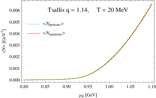
We observe in Fig. 2 (left) that for both and we obtain lines with similar shapes, but is always lower than . The ratio between both temperatures is practically constant up to , as can be seen in Fig. 2 (right), and a consequence is that the curve which results from the multiplication of the results with by a constant factor equal to 3.65 (in the energy per particle case) almost reproduces the result with BG statistics in Fig. 2 (left). This constant factor is of the order of 5 when using the entropy criterium. In the following we will restrict our discussion to the results obtained with the energy per particle hypothesis. In this case the chemical freeze-out lines spam over the region of with the same maximum value for , corresponding to a null critical temperature. Near this maximum value the relation tends to be close to . The curves in Fig. 2 (left) show an inflection for which is related to the sharp increase in the baryon density as the baryonic chemical potential approaches the proton/neutron mass . This increase is displayed in Fig. 3, where we plot the proton and neutron densities as a function of in Tsallis statistics. A similar behavior is observed in Boltzmann-Gibbs statistics.
For the effective temperature is for , which is not in agreement with the value found in the analysis of the -distributions [18]. This disagreement can be related to the value adopted for , which still must be checked by analysis of experimental data with the non extensive statistic. In order to provide an estimate of the sensitivity of the value of when changing it is worth mentioning that the effective temperature for a slightly smaller value of the entropic index, , is , which is in agreement with that reference.
The transition line determines the region where the confined states exist (below the line), and the region where one expects to find the quark-gluon plasma (above the line).
 |
 |
 |
 |
 |
 |
 |
 |
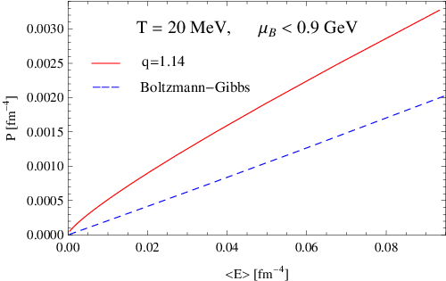
In Fig. 4 (left) we plot the pressure as a function of the temperature for the chemical potentials fixed at the value for the baryonic chemical potential and for all mesons with and . We observe that the pressure increases faster in the non extensive case, , than in the extensive one, . In Fig. 4 (right) we show the results for the pressure as a function of the energy density for . Also here we observe that the pressure increases faster in the case of in comparison with the case . We show in Fig. 5 the pressure as a function of the temperature and chemical potential in the regime and , in Boltzmann-Gibbs (left) and in Tsallis with (right). The more rapid growth of the pressure in Tsallis statistics in comparison with Boltzmann-Gibbs is clear for all the values of displayed, but this effect becomes much stronger for , see also Fig. 4 (left). From Figs. 4 and 5 one can conclude that the EOS for hadronic matter obtained with the Tsallis statistics is harder than the one obtained from the BG case.
Up to now we have studied the equation of state including the spectrum of hadrons in Table 1 and 2. It would be interesting to analyze also the case in which only protons, neutrons and possibly pions contribute to the equation of state, all of them with nonzero chemical potential. We have studied the finite pion chemical potential in two different cases: a) , b) ; and , in both cases. These values are relevant for the study of protoneutron stars [42]. The phase transition lines in Boltzmann-Gibbs and in Tsallis statistics in the regime of high baryonic chemical potential are plotted in Fig. 6. Note that the effect of finite pion chemical potential is to increase the transition line to higher values of temperature, and the curves with and coincide, as we have not introduced electrons in the computation. We show in Fig. 7 the result for the equation of state considering zero and finite pion chemical potential. The effect of pions is to increase the values for the pressure with respect to the case with only protons and neutrons. When considering a nonzero value for the pion chemical potential this leads to a noticeable effect on the EOS, as it becomes harder either in Boltzmann-Gibbs or in Tsallis statistics, see Fig. 7 (right).
V Conclusions
In this work we developed the non extensive thermodynamics for an ideal quantum gas for both bosons and fermions from the partition function defined here for the first time. Then we showed that the partition function and the thermodynamics derived from it is equivalent to the thermodynamics derived from the entropy proposed by Conroy, Miller and Plastino [26], and also by Cleymans and Worku [21] when . For and for fermions some inconsistencies of previous references were addressed, and our result is fully thermodynamically consistent. In the limit of high energies, the partition function is in accordance with that proposed in Ref. [17], and thus the partition function defined here is self-consistent in the sense proposed by Hagedorn.
Some thermodynamical functions are derived from the partition function for hadronic systems with different values of chemical potentials. Particularly we analyze how pressure and energy densities vary when the entropic index or the chemical potentials vary, and we obtain the chemical freeze-out line by using two different hypotheses. A discussion about a discontinuity observed in the first derivatives of the partition function is done for the first time.
The results presented in this work can be applied to stellar matter, where high pressures are necessary to compensate for the gravitational force so that protoneutron star stability and correct macroscopic properties are attained. This study is performed in other work [42], and the results compared with the ones existing in the literature [43].
Acknowledgments
This work has been supported by Plan Nacional de Altas Energías (FPA2011-25948), Junta de Andalucía grant FQM-225, Generalitat de Catalunya grant 2014-SGR-1450, Spanish MINECO’s Consolider-Ingenio 2010 Programme CPAN (CSD2007-00042), Centro de Excelencia Severo Ochoa Programme grant SEV-2012-0234, by CNPq (Brazil) and FAPESC (Brazil) under project 2716/2012,TR 2012000344, and FAPESP (Brazil) under grant 2013/24468-1. A.D. acknowledges the support from CNPq under grant 305639/2010-2. E.M. would like to thank the Instituto de Física of the Universidade de São Paulo for their hospitality and support during the completion of parts of this work. The research of E.M. is supported by the Juan de la Cierva Program of the Spanish MINECO grant JCI-2010-06699.
References
- [1] C. Tsallis, J. Stat. Phys. 52 (1988) 479.
- [2] http://tsallis.cat.cbpf.br/biblio.htm.
- [3] I. Bediaga, E.M.F. Curado e J.M. de Miranda, Physica A 286 (2000) 156.
- [4] R. Hagedorn, Nuovo Cimento Suppl. 3 (1965) 147.
- [5] B. Abelev et al. (ALICE Collaboration), Phys. Lett. B 717, 162 (2012).
- [6] B. Abelev et al. (ALICE Collaboration), Eur. Phys. J. C 72 (2012) 2183.
- [7] K. Aamodt et al. (ALICE Collaboration), Eur. Phys. J. C 71 (2011) 1655.
- [8] V. Khachatryan et al. (CMS Collaboration), JHEP 05 (2011) 064.
- [9] G. Aad et al. (ATLAS Collaboration), Nucl. Phys. B 850 (2011) 387-444.
- [10] R. Hagedorn, Lect. Notes Phys. 221, 53 (1985).
- [11] N. O. Agasian, Phys. Lett. B 519, 71 (2001).
- [12] W. Broniowski, W. Florkowski and L. Y. .Glozman, Phys. Rev. D 70, 117503 (2004).
- [13] A. Tawfik, Phys. Rev. D 71, 054502 (2005).
- [14] E. Megias, E. Ruiz Arriola and L. L. Salcedo, Phys. Rev. Lett. 109, 151601 (2012).
- [15] E. Megias, E. Ruiz Arriola and L. L. Salcedo, Nucl. Phys. Proc. Suppl. 234, 313 (2013).
- [16] E. Megias, E. Ruiz Arriola and L. L. Salcedo, Phys. Rev. D 89, 076006 (2014).
- [17] A. Deppman, Physica A 391 (2012) 6380. See also A. Deppman, Physica A 400 (2014) 207–208.
- [18] L. Marques, E. Andrade-II e A. Deppman, Phys. Rev. D 87 (2013) 114022.
- [19] I. Sena e A. Deppman, Eur. Phys. J. A 49 (2013) 17.
- [20] I. Sena e A. Deppman, AIP Conf. Proc. 1520, (2013) 172.
- [21] J. Cleymans e D. Worku, J. Phys. G: Nucl. Part. Phys. 39 (2012) 025006.
- [22] A. Deppman, J. Phys. G: Nucl. Part. Phys. 41, 055108 (2014).
- [23] N. K. Glendenning, Compact Stars, Springer-Verlag, New-York, (2000).
- [24] P. Haensel, A. Y. Potekhin, D. G. Yakovlev: Neutron Stars, Equation Of State And Structure, Springer, New York (2006).
- [25] B. D. Serot and J. D. Walecka, Adv. Nucl. Phys. 16, 1 (1986); J. Boguta and A. R. Bodmer, Nucl. Phys. A 292, 413 (1977).
- [26] J.M. Conroy, H.G. Miller and A.R. Plastino, Physics Letters A 374 (2010) 4581–4584.
- [27] A.M. Teweldeberhan, A.R. Plastino and H. Miller, Physics Letters A 343 (2005) 71-78.
- [28] J. Cleymans, K. Redlich, Phys. Rev. Lett. 81, 5284 (1998)
- [29] J. Cleymans, K. Redlich, Phys. Rev. C 60 (1999) 054908.
- [30] P. Braun-Munzinger and J. Stachel, J. Phys. G: Nucl. Part. Phys. 28 (2002) 1971.
- [31] V. Magas and H. Satz, Eu. Phys. J. C 32, 115 (2003).
- [32] A. Tawfik, Nucl. Phys. A 764 (2006) 387.
- [33] A. Tawfik, Nucl. Phys. A 922 (2014) 225.
- [34] Sourendu Gupta, Xiaofeng Luo, Bedangadas Mohanty, Hans Georg Ritter, Nu Xu, Science 332:1525-1528, 2011
- [35] J. Beringer et al., Phys. Rev. D 86 (2012) 010001.
- [36] G. Endrodi, arXiv:1311.0648.
- [37] S. Ejiri, Eur. Phys. J. A (2013) 49.
- [38] J. Cleymans, H. Oeschler, K. Redlich and S. Wheaton, Phys. Rev. C 73, 034905 (2006).
- [39] A. Andronic, P. Braun-Munzinger and J. Stachel, Nucl. Phys. A 772, 167 (2006).
- [40] G. Agakishiev et al. [HADES Collaboration], Eur. Phys. J. A 47, 21 (2011).
- [41] X. Lopez, N. Herrmann, P. Crochet, A. Andronic, V. Barret, Z. Basrak, N. Bastid and M. L. Benabderrahmane et al., Phys. Rev. C 76, 052203 (2007).
- [42] D. P. Menezes, A. Deppman, E. Megias and L. B. Castro, arXiv:1410.2264 [nucl-th].
- [43] A. Lavagno and D. Pigato, Eur. Phys. J. A (2011) 47: 52; G. Gervino, A. Lavagno and D. Pigato, J. Physics: Conference Series 442 (2013) 012065.