Simple geodesics and Markoff quadsThanks: This work was supported by the Australian Research Council grant DP1094328.

Closed geodesics on hyperbolic surfaces have extremely rich properties, arising in geometry, topology and number theory, and this is particularly true of simple (that is: non-self-intersecting) closed geodesics. The central objects of our study are simple closed geodesics on 3-cusped projective planes. We describe an algorithm for generating these geodesics and their lengths, and use this algorithm to study systoles, McShane identities and simple length spectra of 3-cusped projective planes.

Systoles: The systole $\mathop{\rm sys}\nolimits(M)$ of a Riemannian manifold $M$ is the length of its shortest essential closed curve which is necessarily a simple closed geodesic. First mentioned in [23], Loewner’s torus inequality gives the following relationship between the systole $\mathop{\rm sys}\nolimits(T)$ of a Riemannian torus $T$ and its surface area $\mathop{\rm Vol}\nolimits(T)$:

equality is realised for tori obtained by gluing opposite sides of regular hexagons. Since then, systolic inequalities have been obtained for other surfaces and higher dimensional manifolds such as Gromov’s inequality [8] which holds for a large class of Riemannian manifolds.

More recently, there has been growing interest in systolic hyperbolic geometry. For example, for orientable hyperbolic surfaces $X$ with $n\geq 2$ cusps and/or boundary components [26]:

Hyperbolic systolic inequalities do not require a volume term on the right, because the area of a hyperbolic surface $X$ is topologically determined: it is $2\pi|\chi(X)|$.

McShane identities: A McShane identity may be thought of as a type of trigonometric identity for hyperbolic surfaces. It is usually a sum over functions of lengths of simple closed geodesics on a punctured/bordered hyperbolic surface. In particular, the structure of this sum is independent of the hyperbolic structure on the surface.

McShane proved the first such identity in his doctoral dissertation [16]. Denote the collection of simple closed geodesics on a 1-cusped torus $X_{1,1}$ by $\mathcal{S}_{1,1}$, then:

where $\ell_{\gamma}$ denotes the length of the simple closed geodesic $\gamma$. Each term in the above series corresponds to the probability that a geodesic launched from the cusp on $X_{1,1}$, up to its first point of self-intersection, does not intersect $\gamma$. McShane identities for other hyperbolic surfaces and quasi-Fuchsian representations have steadily followed [1, 9, 10, 12, 16, 17, 19, 21, 28].

Simple length spectra: Given a Riemannian surface, its length spectrum is the multiset of lengths of closed geodesics on the surface. The Selberg trace formula interprets the length spectrum in terms of the spectrum of the Laplace-Beltrami operator [27], and can be used to show that the number of closed geodesics of length less than $L$ on an orientable hyperbolic surface grows exponentially.

The simple length spectrum is the multiset of lengths of simple closed geodesics. Simple closed geodesics are relatively rare among closed geodesics. The growth rate of the simple length spectrum on an orientable hyperbolic surface is only polynomial in $L$. This was first proven using combinatorial arguments [18, 24]. Mirzakhani gives a novel proof of a refinement of this result in [20]: let $\mathcal{S}(X)$ denote the set of simple closed geodesics on a hyperbolic surface $X$, for $L>0$ define

Then, the function $\eta:\mathcal{M}(X)\rightarrow\mathbb{R}_{+}$ defined by taking the limit

is a continuous proper function. Mirzakhani’s proof employs the ergodicity of the mapping class group action on the space of geodesic measured laminations, as well as her calculations of moduli spaces volumes [19] — calculations utilising McShane identities.

Markoff triples: A Markoff triple is a solution $(x,y,z)\in\mathbb{C}^{3}$ to the equation:

The hypersurface in $\mathbb{C}^{3}$ defined by (4) is the relative character variety of the fundamental group of the once-punctured torus. In particular, this gives a real analytic diffeomorphism between the set of positive real Markoff triples and the Fuchsian component of the character variety — a model for the Teichmüller space of hyperbolic 1-cusped tori.

The following transformations:

take one Markoff triple to another. In particular, these transformations (5) generate the extended mapping class group of the punctured torus, and describe its action on the corresponding relative character variety. For Fuchsian characters, any triple $(x,y,z)\in\mathbb{R}^{3}_{+}$ consists of $2\cosh(\frac{1}{2}\cdot)$ of the lengths of an ordered triple of simple closed geodesics on a particular 1-cusped torus $X$. One is thus able to generate the entire simple length spectrum of $X$ by applying sequences of the transformations in (5) to $(x,y,z)$.

This relationship between positive real Markoff triples and the simple length spectra of hyperbolic 1-cusped tori was first exploited in [6]. In [3], Bowditch uses a generalisation of this correspondence to derive a sharp systolic inequality for quasi-Fuchsian representations of 1-cusped tori, and also to establish a quasi-Fuchsian generalisation of McShane’s original identity. The length generation algorithm can also be used to prove that quasi-Fuchsian representations of the punctured torus group have $L^{2}$ simple length growth rates [11].

The hypersurface in $\mathbb{C}^{4}$ defined by (6) is the relative character variety of the fundamental group of the thrice-punctured projective plane $N_{1,3}$. In other words, we have the following bijective correspondence:

Characters of Fuchsian and quasi-Fuchsian representations are of special importance because they respectively arise as monodromy representations of hyperbolic surfaces and hyperbolic 3-manifolds. We now describe this relationship and introduce some notation for the rest of the paper.

Fuchsian: Given a Fuchsian representation of the fundamental group of a (possibly non-orientable) surface $S$

the discrete subgroup $\rho(\pi_{1}(S))$ acts properly discontinuously on the hyperbolic plane $\mathbb{H}$ by (possibly orientation reversing) isometries. The quotient $\mathbb{H}/\rho(\pi_{1}(S))$ is a complete hyperbolic surface homeomorphic to $S$, and we denote it by $X_{\rho}$. By identifying the universal cover of $S$ with $\mathbb{H}$, Fuchsian representations induce a homeomorphism $h_{\rho}:S\rightarrow X_{\rho}$, canonical up to homotopy.

Quasi-Fuchsian: Similarly, for a strictly quasi-Fuchsian representation

the discrete subgroup $\rho(\pi_{1}(S))$ acts properly discontinuously on $\mathbb{H}^{3}$ by orientation preserving isometries. The quotient space $\mathbb{H}^{3}/\rho(\pi_{1}(S))$ is an orientable complete hyperbolic 3-manifold homeomorphic to $(0,1)\times S$, and we also denote it by $X_{\rho}$. In analogy to the Fuchsian case, quasi-Fuchsian representations induce a canonical (up to homotopy) embedding $h_{\rho}:S\hookrightarrow X_{\rho}$.

Length functions on character varieties: Given a simple closed curve $\gamma$ on $S$, there is a unique simple closed geodesic on $X_{\rho}$ homotopy equivalent to $h_{\rho}(\gamma)$. This allows one to define a function $\ell_{\gamma}(\cdot)$ on the space of quasi-Fuchsian representations of $\pi_{1}(S)$ by taking the complex length of the unique closed geodesic homotopy equivalent to $h_{\rho}(\gamma)$ in $X_{\rho}$. The complex length of a geodesic has real and imaginary parts respectively given by its geometric length and the angle of twisting of the normal bundle around the closed geodesic.

Take note that theorem 2 is a series over $\mathop{\rm Sim}\nolimits_{2}(N_{1,3})$, the set of two-sided simple closed curves on $N_{1,3}$, rather than over the collection $\mathcal{S}_{2}(X_{\rho})$ of two-sided simple closed geodesics on the hyperbolic 3-manifold $X_{\rho}$. This is because for non-Fuchsian representations $\rho$, the geodesic representatives of $\mathop{\rm Sim}\nolimits_{2}(N_{1,3})$ constitutes only a subset of $\mathcal{S}_{2}(X_{\rho})$. Similarly, we consider the subset of the simple length spectrum of a quasi-Fuchsian representation $\rho$ corresponding to the set $\mathop{\rm Sim}\nolimits_{1}(N_{1,3})$ of one-sided simple closed curves on $N_{1,3}$, and study the growth rate of the following quantity:

When $\rho$ is Fuchsian, the value of $s_{\rho}(L)$ is equal to the number $s_{X_{\rho}}(L)$ of geodesics on $X_{\rho}$ below length $L$.

The authors are grateful to Craig Hodgson for useful conversations, to Andrew Elvey-Price and Greg McShane for helping us to improve the bounds in Theorem 3, and to Ser Peow Tan and Hengnan Hu for conversations about their work.

The fundamental group $\pi_{1}(N_{1,3})$ for thrice-punctured projective planes is the free froup $F_{3}$ of rank 3. Any representation $\rho:\pi_{1}(N_{1,3})\rightarrow\mathop{\rm PSL}\nolimits(2,\mathbb{C})$ of a free group admits a lift to a representation

The character $\xi=\mathop{\rm tr}\nolimits\tilde{\rho}$ completely determines the geometry of $X_{\rho}$, and so we consider the $\mathop{\rm PSL}\nolimits(2,\mathbb{C})$-character variety of

We set $A_{i}\in\mathop{\rm SL}\nolimits(2,\mathbb{C})$ to denote the matrix $\tilde{\rho}(\alpha_{i})$.

Goldman showed [7] that any $\mathop{\rm SL}\nolimits(2,\mathbb{C})$-character is determined by the values

Thus, the $\mathop{\rm SL}\nolimits(2,\mathbb{C})$-character variety for $F_{3}$ may be embedded as a subvariety in $\mathbb{C}^{7}$. In particular, the character variety is a hypersurface defined by Fricke’s relation [13] for matrices in $\mathop{\rm GL}\nolimits(2,\mathbb{C})$ — in fact for $\mathop{\rm PGL}\nolimits(2,\mathbb{C})$ since the identity is homogeneous: given three matrices $A_{1},A_{2},A_{3}\in\mathop{\rm GL}\nolimits(2,\mathbb{C})$, set $A_{0}=A_{1}A_{2}A_{3}$. Then,

The symmetric sum here is taken over all possible choices for $\{i,j,k\}=\{1,2,3\}$; the factor of $\tfrac{1}{2}$ in (9) compensates for indices such as $(i,j,k)=(1,2,3)$ and $(1,3,2)$ giving repeated terms. The proof of (9) uses the fact that it extends to a relation on $M(2,\mathbb{C})$ which is quadratic in each entry of $A_{i}$.

For our purposes, we study the relative character variety consisting of type-preserving representations of $F_{3}$ (i.e. where peripheral elements are parabolic). The peripheral elements of the thrice-punctured projective plane are conjugate to $A_{1}A_{2}$, $A_{2}A_{3}$, $A_{3}A_{1}$ or their inverses, so we impose the constraints:

Moreover, instead of considering $\mathop{\rm SL}\nolimits(2,\mathbb{C})$ characters, we consider characters of $\mathop{\rm SL}\nolimits^{\pm}(2,\mathbb{C})$-representations such that

This choice may seem a little unnatural in $\mathop{\rm GL}\nolimits(2,\mathbb{C})$ since we can simply replace $A_{k}$ by $iA_{k}$ to recover a $\mathop{\rm SL}\nolimits(2,\mathbb{C})$ character. We choose $\det A_{k}=-1$ because it is natural when restricting to Fuchsian representations. With this normalisation, Fuchsian representations $\rho:F_{3}\rightarrow\mathop{\rm PSL}\nolimits^{\pm}(2,\mathbb{R})$ have real coefficients. Note that when lifting from $\mathop{\rm PSL}\nolimits^{\pm}(2,\mathbb{R})$ to $\mathop{\rm SL}\nolimits^{\pm}(2,\mathbb{R})$, one-sided curves necessarily have negative determinant.

Since $\det A_{i}=-1$, then $A_{i}$ and $A_{i}^{-1}$ are not conjugate (as they would be in $\mathop{\rm SL}\nolimits(2,\mathbb{C})$), we need to specify orientations on the simple closed curves representing their conjugacy classes. In figure 3,

we see that there is a choice of orientation for simple close curves representing $A_{1}$, $A_{2}$ and $A_{3}$ (anticlockwise) so that the curves representing $A_{1}A_{2}A_{3}$ and $A_{1}A_{3}A_{2}$ are simple. These are the two choices of $A_{1}^{\pm 1}A_{2}^{\pm 1}A_{3}^{\pm 1}$ (up to conjugation and inversion) which are simple, and we choose

Set $a=\mathop{\rm tr}\nolimits A_{1}$, $b=\mathop{\rm tr}\nolimits A_{2}$, $c=\mathop{\rm tr}\nolimits A_{3}$, $d=\mathop{\rm tr}\nolimits A_{4}$ and $d^{\prime}=\mathop{\rm tr}\nolimits A_{4}^{\prime}$, then (9) reorganises to yield (6):

which means that $(a,b,c,d)$ and $(a,b,c,d^{\prime})$ are Markoff quads. In addition, since $d$ and $d^{\prime}$ are the roots of the polynomial

the following identities must hold:

It should be noted that these are precisely the sum and product relations in [7].

Successive applications of equation (15) enables one to generate the trace (and hence the length) of every one-sided simple closed homotopy class on $X$. We now explain how to generate the traces of all of the 2-sided simple closed homotopy classes.

Any two one-sided simple closed curves ${\color[rgb]{1,0,0}\gamma_{i}},{\color[rgb]{0,0,1}\gamma_{j}}$ intersecting exactly once live inside an embedded punctured Möbius strip, as depicted in Figure 4. They uniquely induce a two-sided simple closed curve as a boundary component (with the other boundary component peripheral in $N_{1,3}$).

The following trace identity in $\mathop{\rm GL}\nolimits(2,\mathbb{C})$

relates the complex lengths of peripheral curves $\alpha$ and $\beta$ of a punctured Möbius strip to the complex lengths of ${\color[rgb]{1,0,0}\gamma_{i}}$ and ${\color[rgb]{0,0,1}\gamma_{j}}$:

Since any 2-sided geodesic on a 3-cusped projective plane necessarily bounds a pair of pants, equation (17) allows one to obtain the length of any 2-sided simple closed geodesic.

Equations (15) and (16) give us an algorithm to generate the entire length spectrum of a 3-cusped projective plane, starting from a corresponding Markoff quad. The combinatorics of this algorithm can be stored in terms of the curve complex of $N_{1,3}$.

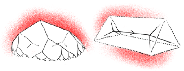
Consider the geometric realisation of the abstract simplicial complex $\Omega^{*}$ with its $n$-simplices given by subsets of $n+1$ distinct homotopy classes of one-sided simple closed curves in $N_{1,3}$ that pairwise intersect once. Identifications of simplices as the faces of higher dimensional simplicies is given by inclusion. This is a pure simplicial $3$-complex, and its $1$-skeleton has been previously described by Scharlemann [25] as being the 1-skeleton of the cell complex formed from a tetrahedron by repeated stellar subdivision of the faces, but not the edges.

The curve complex $\Omega$ that we’re concerned with is the dual of $\Omega^{*}$. The decision to take the dual accords with Bowditch’s conventions in [3, 4]. We now describe and assign notation for the cells of $\Omega$.

The vertices, or $0$-cells of $\Omega$ are:

The edges, or $1$-cells of $\Omega$ are:

Observe that each edge may be interpreted as a flip from one $0$-cell to another. Hence, the 1-skeleton of $\Omega$ is a 4-regular tree (i.e. each vertex has degree 4). Further, the connectedness of this cell-complex described in [25, Theorem 3.1] means that flips generate all possible $0$-cells, and hence all one-sided simple closed geodesics.

The faces, or $2$-cells of $\Omega$ are:

It follows from the observation in the previous subsection regarding punctured Möbius strips embedded in $S$ that each face represents a unique homotopy class of essential, non-peripheral two-sided simple closed curves on $N_{1,3}$.

The 3-cells $\Omega^{3}$ of $\Omega$ are:

We later sometimes denote $3$-cells by capital letters, and use:

to denote the collection of oriented edges of $\Omega$. In particular, $\{\alpha,\beta,\gamma;\delta^{\prime}\rightarrow\delta\}$ points from $\{\delta^{\prime}\}$ to $\{\delta\}$. Figure 5 illustrates the local geometry of an oriented edge.

Given a representation $\rho:F_{3}\to\mathop{\rm GL}\nolimits(2,\mathbb{C})$ satisfying the trace condition (12) and the determinant condition (13), we use Greek letters for simple closed curves and the corresponding Latin letters for the trace of the image of any homotopy class it defines. We decorate $\Omega$ with trace data by assigning to every 3-cell $\{\alpha\}\in\Omega^{3}$ its corresponding trace $\mathop{\rm tr}\nolimits\rho(\alpha)=a$ thus defining a function:

A Markoff map induced from $\rho$ may be thought of as the character corresponding to $\rho$ restricted to one-sided simple closed homotopy classes. Our previous discussions in subsection 2.1 mean that the data carried by a Markoff map suffices to recover the whole character.

We introduce the language of Markoff maps to allude to Bowditch’s work [3, 4]; lower-dimensional simplices in $\Omega$ may be interpreted as mnemonics for encoding the following relations:

Vertex relation: for $\{\alpha,\beta,\gamma,\delta\}\in\Omega^{0}$, (6) is equivalent to:

where $a=\mathop{\rm tr}\nolimits\rho(\alpha)$, $b=\mathop{\rm tr}\nolimits\rho(\beta)$, $c=\mathop{\rm tr}\nolimits\rho(\gamma)$ and $d=\mathop{\rm tr}\nolimits\rho(\delta)$. Note that the set of values of any four 3-cells which meet at a vertex corresponds to a Markoff quad.

Edge relation: an edge $e=(\alpha,\beta,\gamma)\in\Omega^{1}$ lies in the intersection of the two 0-cells $(\alpha,\beta,\gamma,\delta)$ and $(\alpha,\beta,\gamma,\delta^{\prime})$, and (15) yields:

where $d^{\prime}=\mathop{\rm tr}\nolimits\rho(\delta^{\prime})$ and the others are as previously defined. Since each edge joins two vertices, the edge relation therefore tells us how to flip from one Markoff quad to another.

Face relation: given $\{\alpha,\beta\}\in\Omega^{2}$ and $\epsilon$ the unique non-peripheral two-sided simple closed homotopy class disjoint from $\alpha$ and $\beta$, from (16) we have:

where $a=\mathop{\rm tr}\nolimits\rho(\alpha)$, $b=\mathop{\rm tr}\nolimits\rho(\beta)$ and $e=\mathop{\rm tr}\nolimits\rho(\epsilon)$.

We stress once again that these three relations allow us to generate the character for $\rho$ from a starting Markoff quad: the vertex and edge relations generate the traces for all the one-sided simple closed curves and the face relation then produces the traces for all of the two-sided simple closed curves.

Thus, we’re led to consider general maps $\phi:\Omega^{3}\rightarrow\mathbb{C}$ satisfying the edge and vertex relations. We call such functions Markoff maps, and let $\Phi$ denote the collection of all Markoff maps. In keeping with our notation for representations, we use Greek and Latin letters respectively for 3-cells (one-sided curves) and their image under some $\phi\in\Phi$.

The above lemma means that the relative character variety that we wish to study may be characterised as the variety of Markoff maps. Among this collection of Markoff maps, we wish to focus on those which correspond to characters of quasi-Fuchsian representations. This leads us to define BQ-Markoff maps:

For $k\geq 0$ and $\phi\in\Phi$, define the set $\Omega_{\phi}^{3}(k)\subseteq\Omega^{3}$ by:

This set allows us to keep track of one-sided simple curves with trace less than $k$, and we similarly define $\Omega^{2}_{\phi}(k)\subset\Omega^{2}$ for two-sided simple curves. Every two-sided simple curve corresponds to a unique 2-cell $\{\alpha,\beta\}$ — the shared face of the two 3-cells $\{\alpha\}$ and $\{\beta\}$. We define:

Note that in using $|ab|$ instead of $|ab-2|$ for the conditions imposed, the set $\Omega^{2}_{\phi}(k)$ doesn’t quite correspond to the set of two-sided simple curves with trace less than $k$. Although we will find this definition more suited to our analysis. In addition, we later focus on the following collection of Markoff maps $\Phi_{BQ}\subset\Phi$:

We show in section 4.2 that these are sufficient conditions to guarantee the existence of a McShane identity for a given Markoff map. These conditions are similar to Bowditch’s BQ-condition, which is a conjectural trace-based characterisation of quasi-Fuchsian representations. The following result shows that our condition is also necessary for quasi-Fuchsian representations of the thrice-punctured projective plane.

The Markoff-Hurwitz equation is given by

Its quadratic nature means its solution variety admits a discrete group action generated by $a_{i}\mapsto a_{1}...a_{n}/a_{i}-a_{i}$, i.e. one can obtain new solutions from old via flips. Previously, only the $n=3$ solutions of the Markoff-Hurwitz equation were known to have a length spectrum interpretation—for a hyperbolic punctured torus. One observation of this paper is the association of solutions of the $n=4$ solutions of the Markoff-Hurwitz equation with Markoff quads, and hence the $\mathop{\rm SL}\nolimits^{\pm}(2,\mathbb{C})$ relative character variety of the thrice-punctured projective plane. The substitution $a=a_{1}^{2}$, $b=a_{2}^{2}$, $c=a_{3}^{2}$, $d=a_{4}^{2}$ into (6) defines a map between solutions $(a_{1},\ldots,a_{4})$ of (27) for $n=4$ and Markoff quads. The map is a quotient by the $Z_{2}^{3}$-action $(a_{1},a_{2},a_{3},a_{4})\mapsto(\pm a_{1},\pm a_{2},\pm a_{3},\pm a_{4})$ (even number of minus signs) on solutions of the Markoff-Hurwitz equation. Flips of Markoff quads correspond to flips of solutions of the Markoff-Hurwitz equation.

The remainder of this section deals with Markoff maps corresponding to Fuchsian representations. From the proof of lemma 4, we see that these are precisely the real Markoff maps. We focus on the Teichmüller component of the real relative character variety, showing that it consists of the positive real Markoff maps.

The Teichmüller space $\mathcal{T}(S)$ of a surface $S$ encodes all the ways of assigning a complete finite-area hyperbolic metric to $S$, up to homotopy. Concretely, it may be expressed as:

where $(X_{1},f_{1})\sim(X_{2},f_{2})$ if and only if

is homotopy equivalent to a hyperbolic isometry. We denote these equivalence classes, or marked surfaces, by $[X,f]$.

An ideal triangulation of $S$ is, up to homotopy, a triangulation of $S$ with vertices at the punctures of $S$. Given a marked surface $[X,f]$, the image $f(\sigma)$ of an arc $\sigma$ on $S$ pulls tight to a unique homotopy equivalent geodesic arc on $X$. Thus, any ideal triangulation on $S$ is represented by an (geodesic) ideal triangulation on $X$ — a maximal collection of simple bi-infinite geodesic arcs with both ends up cusps. For our purposes, we restrict to ideal triangulations $\triangle$ on thrice-punctured projective planes $S$ representable by paths with distinct end points.

Horocycles of length $1$ around a cusp are always simple on a complete hyperbolic surface. Thus, given an ordered ideal triangulation $(\sigma_{1},\sigma_{2},\sigma_{3},\tau_{1},\tau_{2},\tau_{3})$ on $X$, we obtain lengths $(s_{1},s_{2},s_{3},t_{1},t_{2},t_{3})$ of these infinite geodesic arcs truncated at the three length $1$ horocycles bounding cusps $1,2,3$. The $\lambda$-lengths for $X$ with respect to this ordered ideal triangulation is then given by:

In [22], Penner shows that these $\lambda$-lengths form global coordinates on the Teichmüller space of any punctured surface. This is also true for the Teichmüller space of punctured non-orientable surfaces.

The following lemma is a topological correspondence which is promoted to a geometric correspondence below.

These $\lambda$-lengths of an ideal triangulation may be expressed in terms of the Markoff quad of the associated quadruple of one-sided geodesics in $\Omega^{0}$ corresponding to the used to the define these $\lambda$-lengths.

Thus, we may also use positive Markoff quads to globally parametrise the Teichmüller space:

Markoff quads are points on the $\mathop{\rm SL}\nolimits^{\pm}(2,\mathbb{C})$ relative character variety of the thrice-punctured projective plane, which is the hypersurface in $\mathbb{C}^{4}$ defined by equation (6). The transformation (8),

combined with the following even permutations

generate the pure mapping class group of the thrice-punctured projective plane, and specify its action on the corresponding relative character variety. Pure here means that we restrict to elements of the mapping class group that fix punctures.

We construct an explicit homeomorphism $f_{4}:N_{1,3}\rightarrow N_{1,3}$ that takes $(\alpha,\beta,\gamma,\delta)$ to $(\alpha,\beta,\gamma,\delta^{\prime})$. Consider the hexagonal fundamental domain of $N_{1,3}$ obtained by cutting along $\sigma_{1},\sigma_{2}$ and $\sigma_{3}$.

From figure 7, we see that a rotation by $\pi$ of this fundamental domain fixes the labeling of the punctures and fixes each of $\alpha$, $\beta$ and $\gamma$ whilst taking $\alpha$ to $\alpha^{\prime}$. The action of the mapping class $[f_{4}]\in\Gamma(N_{1,3})$ therefore takes the Markoff quad $(a,b,c,d)$ corresponding to a marked surface $[X,f]$ to

that is: $[f_{4}]$ corresponds to a flip in the fourth entry. By symmetry, there are four flips $[f_{1}],[f_{2}],[f_{3}],[f_{4}]\in\Gamma(N_{1,3})$ which flip the corresponding entries of $(a,b,c,d)$. Let $F\leq\Gamma(N_{1,3})$ denote the subgroup generated by these four flips.

References

- [1] Hirotaka Akiyoshi, Hideki Miyachi, and Makoto Sakuma. Variations of McShane’s identity for punctured surface groups. In Spaces of Kleinian groups, volume 329 of London Math. Soc. Lecture Note Ser., pages 151–185. Cambridge Univ. Press, Cambridge, 2006.
- [2] Arthur Baragar. The exponent for the Markoff-Hurwitz equations. Pacific J. Math., 182(1):1–21, 1998.
- [3] B. H. Bowditch. A proof of McShane’s identity via Markoff triples. Bull. London Math. Soc., 28(1):73–78, 1996.
- [4] B. H. Bowditch. Markoff triples and quasi-Fuchsian groups. Proc. London Math. Soc. (3), 77(3):697–736, 1998.
- [5] J. W. S. Cassels. An introduction to Diophantine approximation. Cambridge Tracts in Mathematics and Mathematical Physics, No. 45. Cambridge University Press, New York, 1957.
- [6] Harvey Cohn. Approach to Markoff’s minimal forms through modular functions. Ann. of Math. (2), 61:1–12, 1955.
- [7] William M. Goldman. Trace coordinates on Fricke spaces of some simple hyperbolic surfaces. In Handbook of Teichmüller theory. Vol. II, volume 13 of IRMA Lect. Math. Theor. Phys., pages 611–684. Eur. Math. Soc., Zürich, 2009.
- [8] Mikhael Gromov. Filling Riemannian manifolds. J. Differential Geom., 18(1):1–147, 1983.
- [9] Hengnan Hu. Identities on hyperbolic surfaces, group actions and the Markoff-Hurwitz equations. PhD thesis, National University of Singapore, August 2013.
- [10] Yi Huang. A mcshane-type identity for closed surfaces. preprint (to appear in the Nagoya Mathematical Journal), 2012. arXiv:1203.3860.
- [11] Yi Huang. Moduli Spaces of Surfaces. PhD thesis, The University of Melbourne, June 2014.
- [12] Feng Luo and Ser Peow Tan. A dilogarithm identity on moduli spaces of curves. J. Differential Geom., 97(2):255–274, 2014.
- [13] Wilhelm Magnus. Rings of Fricke characters and automorphism groups of free groups. Math. Z., 170(1):91–103, 1980.
- [14] Sara Maloni, Frederick Palesi, and Ser Peow Tan. On the character variety of the four-holed sphere. preprint, 2014. arXiv:1304.5770.
- [15] André Markoff. Sur les formes quadratiques ternaires indéfinies. Math. Ann., 56(2):233–251, 1902.
- [16] Greg McShane. A remarkable identity for lengths of curves. PhD thesis, University of Warwick, May 1991.
- [17] Greg McShane. Simple geodesics and a series constant over Teichmuller space. Invent. Math., 132(3):607–632, 1998.
- [18] Greg McShane and Igor Rivin. Simple curves on hyperbolic tori. C. R. Acad. Sci. Paris Sér. I Math., 320(12):1523–1528, 1995.
- [19] Maryam Mirzakhani. Simple geodesics and Weil-Petersson volumes of moduli spaces of bordered Riemann surfaces. Invent. Math., 167(1):179–222, 2007.
- [20] Maryam Mirzakhani. Growth of the number of simple closed geodesics on hyperbolic surfaces. Ann. of Math. (2), 168(1):97–125, 2008.
- [21] Paul Norbury. Lengths of geodesics on non-orientable hyperbolic surfaces. Geom. Dedicata, 134:153–176, 2008.
- [22] R. C. Penner. The decorated Teichmüller space of punctured surfaces. Comm. Math. Phys., 113(2):299–339, 1987.
- [23] P. M. Pu. Some inequalities in certain nonorientable Riemannian manifolds. Pacific J. Math., 2:55–71, 1952.
- [24] Igor Rivin. Simple curves on surfaces. Geom. Dedicata, 87(1-3):345–360, 2001.
- [25] Martin Scharlemann. The complex of curves on nonorientable surfaces. J. London Math. Soc. (2), 25(1):171–184, 1982.
- [26] Paul Schmutz. Congruence subgroups and maximal Riemann surfaces. J. Geom. Anal., 4(2):207–218, 1994.
- [27] A. Selberg. Harmonic analysis and discontinuous groups in weakly symmetric Riemannian spaces with applications to Dirichlet series. J. Indian Math. Soc. (N.S.), 20:47–87, 1956.
- [28] Ser Peow Tan, Yan Loi Wong, and Ying Zhang. Generalizations of McShane’s identity to hyperbolic cone-surfaces. J. Differential Geom., 72(1):73–112, 2006.