Static weak dipole moments of the lepton via renormalizable scalar leptoquark interactions
Abstract
The weak dipole moments of elementary fermions are calculated at the one-loop level in the framework of a renormalizable scalar leptoquark model that forbids baryon number violating processes and so is free from the strong constraints from experimental data. In this model there are two scalar leptoquarks accommodated in an doublet: one of such leptoquarks is non-chiral and has electric charge of , whereas the other one is chiral and has electric charge . In particular, a non-chiral leptoquark contributes to the weak properties of an up fermion via a chirality flipping-term proportional to the mass of the virtual fermion and can also induce a non-zero weak electric dipole moment provided that the leptoquark couplings are complex. The numerical analysis is focused on the weak properties of the lepton since they offer good prospects for their experimental study. The constraints on leptoquark couplings are briefly discussed for a non-chiral leptoquark with non-diagonal couplings to the second and third fermion generations, a third-generation non-chiral leptoquark, and a third-generation chiral leptoquark. It is found that although the chirality-flipping term can enhance the weak properties of the lepton via the top quark contribution, such an enhancement would be offset by the strong constraints on the leptoquark couplings. So, the contribution of scalar leptoquarks to the weak magnetic dipole moment of the lepton are smaller than the standard model (SM) contributions but can be of similar size than those arising in some SM extensions. A non-chiral leptoquark can also give contributions to the weak electric dipole moment larger than the SM one but well below the experimental limit. We also discuss the case of the off-shell weak dipole moments and for completeness analyze the behavior of the electromagnetic properties.
I Introduction
The study of the static electromagnetic properties of charged leptons has long played a central role in experimental particle physics. The magnetic dipole moment (MDM) and the electric dipole moment (EDM), which can only arise for spinning particles, have drawn as much attention as that devoted to other particle properties. Although the electron MDM, , has been an instrumental probe of quantum electrodynamics, any new physics contribution to is too small to be at the reach of detection, so the experimental measurements are commonly employed to determine the value of the fine structure constant rather than to look for evidences of new physics. A different scenario arises in the case of the muon MDM, , which receives sizeable contributions from all the sectors of the standard model (SM). Even more, can be determined with a very high precision both experimentally and theoretically and thus it has become a powerful benchmark to test the SM with very high accuracy and to search for effects of physics beyond the SM. The most recent experimental determination of , which has reached a precision of 0.7 parts per million [1], leads to a discrepancy with the SM prediction at the level of 3.6 standard deviations:
| (1) |
where the experimental and theoretical errors have been added in quadrature. Although such a discrepancy may be a signal of new physics, a more accurate calculation of the hadronic light-by-light contribution is yet to be obtained.
On the other hand, our knowledge of the lepton electromagnetic properties is still unsatisfactory, which stems from the fact that the lifetime is very short to prevent its interaction with an electromagnetic field from direct measurements. The most stringent current bound on with 95 % C.L., , was obtained by looking for deviations from the SM in the cross section of the process using the data collected by the DELPHI collaboration at the CERN large electron positron (LEP2) collider during the years 1997-2000 [2], while the theoretical SM prediction is [3]. It turns out that a precise measurement of the tau MDM is required as it could confirm or rule out the possibility that the discrepancy is a signal of new physics: the natural scaling of heavy particle effects on a lepton MDM implies that , so if the current discrepancy is interpreted as a new physics effect, we would expect that . Although the SM prediction disagrees with this value, some of its extensions, such as the SeeSaw model [4], the minimal supersymmetric standard model with a mirror fourth generation[5], and unparticle physics [6], predict that lies in the interval of to .
As for the EDM, it represents a useful tool for the study of the discrete symmetry and provides a potential probe to unravel its origin. However, the only EDMs that can be directly measured are those of the neutron, the proton, the deuteron and the muon, whereas the EDM of other particles can only be indirectly determined. Although an experimental signal of an EDM is yet to be detected, the best current upper limits on the electron and muon EDMs come from the study of the thallium EDM [7] and the E821 experiment at Brookhaven [8], respectively:
| (2) | |||||
| (3) |
whereas the experimental detection of the EDM poses the same difficulties as its MDM. Nevertheless, the EDM was searched for in the reaction by the Belle collaboration [9] at the KEK collider. The achieved sensitivity, in units of cm, was
| (4) | |||||
| (5) |
In the SM, the EDM of a lepton is predicted to be negligibly small as it arises at the three-loop level of perturbation theory, which can be a blow for its experimental detection. However, several SM extensions predict sizeable contributions that can be at the experimental reach. Although the short lifetime represents a challenge, this lepton emerges as a natural candidate to search for new physics effects such as a large EDM because of its mass and wide spectrum of decay channels.
The study of physics plays a significant role in factories. For instance, the ill-fated Super accelerator with its 75 ab-1 was expected to measure the EDM with a resolution of cm [10], whereas the expected resolution of the real and imaginary parts of was estimated to be of the order of [11, *O'Leary:2010af]. With a lower planned luminosity, the upgraded Belle II facility at the KEK B-factory will offer unique perspectives for the study of physics in both high precision measurements of the SM parameters and new physics searches. The electromagnetic dipole moments of the lepton may be measured via the radiative leptonic decays () [13]. However, this method is only sensitive to large values of , so a more detailed analysis will determine the feasibility of this proposal.
Contrary to the attention drawn to the static electromagnetic properties of fermions, a lot of work is still necessary to have a better understanding of their weak properties, namely the -conserving weak magnetic dipole moment (WMDM) and the -violating weak electric dipole moment (WEDM), which are the coefficients of dimension-five operators in the effective Lagrangian of the interaction and can be extracted from the following terms of the respective vertex function
| (6) |
where is the gauge boson transferred four-momentum. The WMDM, , and the WEDM, , are defined at the -pole: and . Since and are the coefficients of chirality-flipping terms, they are expected to give contributions proportional to some positive power of the mass of the involved fermion. This allows one to construct observable quantities that can be experimentally proved, but which are particularly suited for heavy fermions, among from which the lepton, the quark, and the quark are the most promising candidates. In particular, a large value of the WEDM of charged fermions would lead to a considerable deviation of the total width from its SM value [14], which can provide an indirect upper limit on the corresponding WEDM. Along these lines, the study of the decay at center-of-mass energies near the resonance represents a promising tool to search for signals of the weak dipole moments of the lepton. This process could allow one to measure and through the transverse and normal polarizations of the leptons [15]. By following this approach, the ALEPH collaboration obtained the current best limit on the WMDM and WEDM, with 95 C.L. [16]:
| (7) | |||||
| (8) | |||||
| (9) | |||||
| (10) |
which were extracted from the data collected at the CERN from 1990 to 1995, corresponding to an integrated luminosity of 155 pb-1. These bounds are far above the SM predictions [17] and cm [14]. However, the CERN large hadron collider (LHC) could open a door for the experimental study of these properties. Along these lines, a study of the and cross sections including anomalous couplings was presented in Ref. [18]. It was found that an analysis at the LHC would allow experimentalists to measure the deviations from the SM and extract constraints on the electromagnetic and weak dipole moments.
The weak properties of a fermion have been studied in several SM extensions, such as models allowing tree-level flavor changing neutral currents [19], the two-Higgs-doublet model (THDM) [20, *GomezDumm:1999tz], the minimal supersymmetric standard model (MSSM) [22, *Hollik:1997vb], the minimal supersymmetric version of the SM with complex parameters [24], and in the context of unparticle physics [6]. Prompted by a recent work [25] on the study of the simplest renormalizable scalar leptoquark models with no proton decay (see also Ref. [26]), we will consider one of such models for our study. This model is interesting as there is a non-chiral leptoquark that could give rise to large contributions to the weak properties of a charged lepton due to a chirality-flipping term. Furthermore, very recently it was shown that such a scalar leptoquark, with mass below 1 TeV, can provide an explanation for the observed branching ratios of the decays [27]. The rest of this article is organized as follows. A brief review on the scalar leptoquark model we are interested in along with the details of the calculation of the weak properties of a fermion is presented in Sec. II. Section III is devoted to the numerical analysis of our results, with particular emphasis to the lepton weak properties, including a short discussion on the case of the off-shell dipole moments. For completeness we will also discuss the electromagnetic properties. The conclusions and outlook are presented in Sec. IV.
II Weak dipole moments of a fermion in scalar leptoquark models
The vanishing of gauge anomalies in the SM due to the interplay of charged fermions hints to a profound link between lepton and quarks in a more fundamental theory, such as the one conjectured long ago by Pati and Salam [28], which gives rise to new leptoquark particles carrying both lepton and baryon numbers. Leptoquark particles can be of scalar or vector type and are also predicted in grand unified theories (GUTs) [29, *Senjanovic:1982ex, *Frampton:1989fu], composite models [32], technicolor models [33, *Hill:2002ap], superstring-inspired models [35, *Hewett:1988xc], etc. For a more comprehensive listing of this class of models along with low-energy constraints, the reader may want to refer to [37, *Hewett:1997ce]. Of special interest are leptoquark models in which baryon and lepton numbers are individually conserved, thereby forbidding any tree-level contribution to proton decay induced by leptoquark couplings to diquarks. As a result, in such models the leptoquark mass can be as light as the electroweak scale, which contrast with some GUT-inspired leptoquark models in which it must lie around the Planck scale in order to avoid a rapid proton decay.
Because of the complexity inherent to leptoquark models, it has been customary to analyze their potential effects in a model-independent fashion via the effective lagrangian approach: the most general dimension-four invariant lagrangian parameterizing both scalar and vector leptoquark couplings satisfying both baryon and lepton number conservation was first presented in [39]. Quite recently, the authors of Ref. [25] brought the attention to the only two minimal renormalizable models where scalar leptoquarks are introduced via a single representation of and in which there is no proton decay induced via tree-level leptoquark exchange. This fact was also stressed previously in Ref. [26]. We will focus on one of this models, dubbed Model I in Ref. [25], and calculate the corresponding contribution to the WMDM and the WEDM of a fermion. Although the WEDM of heavy fermions has already been studied in the context of leptoquark models [40, 41], to our knowledge there is no previous analysis on the behavior of the contributions of leptoquarks to the WMDM. In the model I of Ref. [25] there is a non-chiral leptoquark (it has both left- and right-handed couplings) that gives rise to a chirality-flipping contribution to the electromagnetic and weak properties of a fermion. Such a term is proportional to the internal quark mass and it is worth examining if there is an enhancement in the contribution from a heavy internal fermion.
In the model we are interested in, there is a scalar leptoquark doublet with quantum numbers under the gauge group. For our calculation we only need to consider the following zero-fermion-number effective interaction [39, 42]:
| (11) |
with and .
From the above Lagrangian we obtain the interaction of a lepton-quark pair with two scalar leptoquarks and , with electric charge of and . We write the interaction Lagrangian as
| (12) |
where are the chiral projection operators and are generation indices. The flavor eigenstates were rotated to the mass eigenstates and so the , , and couplings already encompass this information. Notice that while has both left- and right-handed couplings to a charged lepton and an up quark, has only right-handed couplings.
For our purpose we will also need the leptoquark couplings with the photon and the boson, which are extracted from the leptoquark kinetic Lagrangian and can be written in the form
| (13) |
where and . Here is the electrical charge in units of . For completeness, we present the SM interactions of the photon and the gauge boson with a fermion pair:
| (14) |
In particular, we will need below and for the contribution of an up quark to the weak properties. The corresponding Feynman rules can be extracted straightforwardly from the above Lagrangians.

II.1 Weak dipole moments of a fermion
At the one-loop level, the weak properties of the fermion are induced by a scalar leptoquark and a fermion via the Feynman diagrams of Fig. 1. The method of Feynman parameters yields the following results
| (15) | |||||
where we have defined and
| (16) | |||||
| (17) |
The and functions, which stand for the contributions of each one of the Feynman diagram of Fig. 1, can be written as
| (18) |
and
| (19) |
with the auxiliary functions , and defined by , , , and .
As for the weak electric dipole moment of fermion , it can be written in the form
| (20) |
As mentioned above, there is a chirality-flipping term proportional to the internal fermion mass when the leptoquark is non-chiral. Below, we will concentrate on the potential effects of such a leptoquark on the weak properties of the lepton as there can be an important enhancement from the quark contribution.
II.2 Electromagnetic dipole moments of a fermion
For the completeness of our analysis we will also need the contributions from scalar leptoquarks to the static electromagnetic properties of a fermion, which follow easily from our calculation by taking the limit and replacing the couplings by the photon ones. It can be helpful to test the validity of our results. We thus obtain the scalar leptoquark contribution to the magnetic dipole moment and the electric dipole moment of fermion :
| (21) |
and
| (22) |
where
| (23) | |||||
| (24) |
with the and functions given by
| (25) |
| (26) |
The equations can be integrated explicitly in the limit of a very heavy leptoquark, in which case we obtain
| (27) | |||
| (28) |
| (29) | |||
| (30) |
These results are in agreement with previous results for the magnetic [43, 44] and the electric [45] dipole moments induced by scalar leptoquarks. In addition, we present in Appendix A an alternative calculation of the weak and electromagnetic properties of a fermion in terms of Passarino-Veltman scalar functions, which can be used to make a cross-check of our results.
III Numerical analysis
III.1 Leptoquark constraints
In the following analysis we will concentrate on the lepton electromagnetic and weak properties as they offer good prospects for their experimental study. We will consider a charge non-chiral scalar leptoquark as it is expected to give the dominant contribution to the electromagnetic and weak properties of the lepton in the model we are considering. The phenomenology of such a leptoquark has been studied considerably in the past [46, 37, 42] and very recently [25, 27] with constraints from the decay, the muon MDM, lepton flavor violating decays and the EDM. There are strong constraints from low energy physics [46, 37, 42] on leptoquarks that couple to the first-generation fermions, so we will assume a leptoquark that only has non-negligible couplings to fermions of the second and third generations. As for the leptoquark mass, the most stringent constraint on the mass of a third-generation chiral scalar leptoquark, GeV, was obtained from the analysis of the data from the LHC [47]. It was assumed that such a leptoquark decays mainly into a bottom quark and a lepton, such as occurs with the leptoquark. Since it is required that and are mass degenerate or have a small mass splitting to avoid large contributions to the oblique parameters [48], we will assume a leptoquark with a mass larger than 500 GeV.
Below we will focus on three illustrative scenarios and discuss briefly the constraints on the leptoquark coupling constants to present a realistic analysis. We will then analyze the behavior of the electromagnetic and weak properties as a function of the leptoquark mass and also discuss the case of the off-shell dipole moments.
III.1.1 Scenario I: a non-chiral leptoquark with non-diagonal couplings to the second and third fermion generations
We first analyze the scenario in which there exists a non-chiral leptoquark that can have complex non-diagonal couplings to lepton-quark pairs of the second and third generations. In this scenario, the -even electromagnetic and weak properties of the lepton receive the contributions of a non-chiral leptoquark accompanied by the or the quarks and can be enhanced by the chirality-flipping term. In addition, there can be non-zero CP-violating properties. On the negative side, such a leptoquark can give rise to large contributions to the muon MDM and the LFV decay , which in turn can impose strong constraints on the leptoquark couplings. We note that a similar scenario is posed by a scalar singlet leptoquark, such as the one whose behavior was analyzed in [49], which can also be non-chiral but it is known to give dangerous contributions to the proton decay via its diquark couplings.
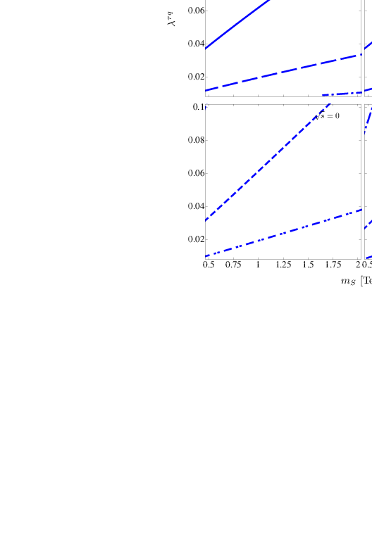
If one assumes that the discrepancy on the muon MDM (1) is due entirely to our scalar leptoquark, the allowed region for its respective contribution, with 95% C.L, is . We assume that either the or the quark contribution is responsible for the discrepancy and obtain the allowed regions on the vs plane with 95 % C.L., which we show in Fig. 2. Although the product is tightly constrained, a less stringent constraint would be obtained if the quark contribution was canceled out by the quark contribution or another new physics contribution.

If the leptoquark has non-diagonal couplings to the second and third generations, the LFV decay can proceed via the Feynman diagrams of Fig. 3. The contribution of leptoquark and quark to the decay amplitude can be written in the form
| (31) |
where the and coefficients are given by
| (32) |
and . This decay was already studied in [50], but we have made our own evaluation for completeness and we present the and functions in Appendix B in terms of Feynman parameter integrals and Passarino-Veltman scalar functions. The respective decay width is given by
| (33) |

As far as the experimental constraints on LFV decays are concerned, quite recently the upper bound on the decay rate for the decay was improved up to by the MEG collaboration [51], but the bounds on the LFV decays are much weaker: BR and [52]. Since both the and vertices, with , enter into the amplitude of the decay, it can only be useful to constrain the product , so a bound on will be largely dependent on .
For simplicity we take () and consider that either the quark or the quark contribution is the only responsible for the discrepancy, i.e. we assume that the , coupling takes on values inside the allowed area shown in Fig. 2. We then obtain the plot of Fig. 4, where we show the allowed region on the vs plane consistent with both the experimental constraints on the muon MDM and the LFV decay . We observe that, in order to explain the discrepancy and be consistent with the decay, the coupling must reach values of the order of about , whereas must reach values one order of magnitude smaller. A word of caution is on order here, the allowed areas of Fig. 4 would alter if the quark contribution was not assumed to be the only responsible for the discrepancy, which in turn could be explained by other contributions of the same model.

III.1.2 Scenario II: a third-generation non-chiral leptoquark
This scenario is similar to the first scenario except that there are no leptoquark-mediated LFV processes and therefore the constraints on the leptoquark couplings are less stringent than in scenario I. The electromagnetic and weak properties of the lepton, which would only receive the contribution of the non-chiral leptoquark and the quark, can still be enhanced by the chirality-flipping term and there can be non-zero -violating properties provided that the leptoquark couplings are complex. Therefore, this scenario can provide the largest values of the electromagnetic and weak properties of the lepton. Constraints on the couplings of such a leptoquark were obtained in Ref. [42] by performing a global fit to the LEP data on physics. It was found that leptoquark couplings of the order of about are allowed provided that the leptoquark mass is of the order of GeV.
III.1.3 Scenario III: a third-generation chiral leptoquark
Although a chiral scalar leptoquark with couplings to fermions of the second-generation would yield a negative contribution to the muon MDM, which is disfavored by the experimental data, such a contribution would vanish for a third-generation leptoquark. In this case the only contributions to the electromagnetic and weak properties of the lepton arise from the chiral leptoquark accompanied by the quark. Apart that this scenario does not induce violating properties, it appears to be unfavorable for large values of the electromagnetic and weak properties as they would be naturally suppressed due to the absence of the chirality-flipping term. Constraints on this class of leptoquarks were obtained in Ref. [53] from the experimental measurement of the partial decays . It was found that a third-generation leptoquark with a mass larger than about 500 GeV and a coupling to the quark and the lepton of electroweak strength are compatible.
III.2 Behavior of the electromagnetic and weak properties of the lepton
In general, the vertex is gauge invariant and gauge independent only when the gauge boson is on its mass shell, therefore the pinch technique was used in [54] to construct gauge-independent electromagnetic and weak dipole form factors. It was argued [55], however, that off-shell form factors are not uniquely defined and so they do not represent observable quantities. In the case of the leptoquark contribution to the weak and electromagnetic dipole moments, there are no internal gauge bosons circulating in the loops and so there is no dependence on the gauge-fixing parameter. Our results for the weak dipole moments can thus be easily generalized for arbitrary squared momentum of the gauge boson by replacing in Eqs. (15) and (20). The electromagnetic dipole form factors follow easily after exchanging the couplings by the photon ones. The resulting quantities can be useful to assess the sensitivity to the effects of leptoquark particles on the dipole form factors, as suggested in the analysis presented in [20] within the framework of the THDM. Below we will analyze the electromagnetic properties for and GeV. On the other hand, the weak properties will be analyzed for and GeV. The values of used for the off-shell gauge bosons are the center-of-mass energies of a factory and the future next linear collider, respectively. Furthermore, in our study below we will consider the interval for and GeV – GeV for , which are in accordance with the bounds from experimental data discussed above. Here represents the leptoquark coupling constants.
We first assume that the leptoquark couplings are real and calculate the following leptoquark contributions to the MDM: that of a non-chiral leptoquark with non-diagonal couplings to a lepton-quark pair of the second and third families and that of a third-generation chiral leptoquark. In the former case there are contributions from the and the quarks, but in the latter there is only a contribution from the quark. We show in Fig. 5 the contours of the MDM in the vs plane for and GeV, with and for the chiral leptoquark (i.e. a left-handed leptoquark), and for the non-chiral leptoquark. Note that the MDM is insensitive to the chirality of the leptoquark, so our results are valid for either a left- or a right-handed leptoquark. As mentioned above, there is an enhancement of the non-chiral leptoquark contribution due to the presence of the chirality-flipping term, but it would be significant only in the case of the quark, whose contribution can reach values slightly above the level for and up to - for . However, in the case of the quark, a small value of the coupling constant would offset the enhancement from the chirality-flipping term and this contribution would be below the level for . In the case of a third-generation chiral leptoquark, although its couplings were of the order of , its contributions would be lower than the contribution of a non-chiral leptoquark accompanied by the quark, provided that the couplings of the non-chiral leptoquark are of the order of . In general, the contribution of a chiral leptoquark is slightly dependent on the quark mass, which is due to the absence of the chirality-flipping term. If the photon goes off-shell, with GeV, there is a slight increase in the real part of and at the same time an imaginary part is developed in the case of the quark contribution since . Such an imaginary part would be slightly smaller than the corresponding real part.
We now show the contours of the in the vs plane in Fig. 6 for and GeV. Again we show the contributions of a non-chiral leptoquark accompanied by the or the quarks and, since the WMDM is sensitive to the chirality of the leptoquark, we now show the contributions of both a left- and a right-handed leptoquark. The largest contribution to the static would arise from a non-chiral leptoquark accompanied by the quark, which can reach the level of for and for , whereas the contribution of a non-chiral leptoquark and the quark is about two orders of magnitude smaller. The latter contribution now develops an imaginary part that is slightly smaller than the real part. As far as the third-generation chiral leptoquark is concerned, the contribution of a left-handed leptoquark can be as large as for GeV and but it is much smaller than the contribution of a non-chiral leptoquark and the quark for smaller and larger . On the other hand, the contribution of a right-handed leptoquark is about one order of magnitude smaller than that of a left-handed one. In general the enhancement due to the chirality-flipping term, which appears only in the non-chiral leptoquark contribution, is less pronounced in the case of the WMDM than in the case of the MDM. When the gauge boson goes off-shell, the real part of the leptoquark contributions to shows a rather similar behavior to that observed in the case of an on-shell gauge boson, but all the contributions develop an imaginary part, which is smaller than the corresponding real part. Although there is an increase in the magnitude of the contributions when the gauge boson goes off-shell, with the largest increase observed in the contribution of a non-chiral leptoquark accompanied by the quark, such an increase is moderate. To summarize, the largest contribution to would arise from a third-generation non-chiral leptoquark even if its couplings were one order of magnitude below than those of a third-generation chiral leptoquark.

We now turn to analyze the -violating properties of the lepton, which can only arise when the leptoquark is non-chiral and its couplings are complex. These properties are proportional to , with the relative phase between the and coupling constants. We first show in Fig. 7 the contours of the contribution to the EDM arising from a non-chiral scalar leptoquark accompanied by the or the quark in the vs plane, for and GeV. We observe that, irrespectively of the value of , the quark contribution to can be as large as - cm for and GeV, but it is two orders of magnitude below for and GeV. On the other hand, the quark contribution is much smaller and can only reach the level of cm even if . Apart from a slight increase in the real part of , the only noticeable difference between the contributions of an on-shell and an off-shell photon is the imaginary part that is developed by the quark contribution, which is smaller than corresponding real part. Finally, we analyze the leptoquark contribution to the WEDM of the lepton, which also is non-vanishing only for a non-chiral leptoquark with complex couplings. In Fig. 8 we show the contours of the contribution of such a leptoquark to in the vs plane for and GeV. As expected, the quark yields the dominant contribution, with values ranging between to cm, whereas the quark contribution is much smaller. When GeV, the behavior of the real part of the contribution of the quark remains almost unchanged with respect to the case of an on-shell gauge boson, though an imaginary part is developed. A more pronounced change is observed in the behavior of the contribution of the quark, which can reach larger values as increases, which is evident by the downward shift of the contour lines as larger values of can be reached for smaller values of .


In summary, the static electromagnetic and weak properties induced by a scalar leptoquark can reach the values shown in Table 1 in the scenarios discussed above, considering values for the coupling constants consistent with the constraints from experimental data. For comparison purpose, we also include the predictions of other extensions of the SM. The reader is referred to the original references for the particular values of the parameters used to obtain these estimates. Notice that there can be additional suppression in these values as we show the largest ones we can expect in every model. In the case of scenario I, although the electromagnetic and weak properties can be enhanced by the contribution of the quark, such an enhancement would likely be offset since the leptoquark couplings are strongly constrained. On the other hand, although the constraints on the leptoquark couplings are less stringent in scenario III than in scenarios I and II, the electromagnetic and weak properties of the lepton are naturally suppressed in such a scenario due to the absence of a chirality-flipping term. In conclusion, scenario II seems to be the one that can give rise to the largest values of the electromagnetic and weak properties as the constraints on the leptoquark couplings are less stringent than in scenario I. Furthermore, in this scenario there can be nonzero -violating properties, which are absent in scenario III. The respective contributions would be, however, smaller than in other SM models such as the MSSM. For an off-shell photon or gauge boson there is no appreciable difference in the order of magnitude of the real part of the electromagnetic and weak dipole moments, though depending on the value of an imaginary part can develop in the case of the quark contribution to the electromagnetic properties and the contribution to the weak dipole moments. Such an imaginary part is absent in the case of on-shell gauge bosons. It is worth mentioning that, for a very heavy scalar leptoquark, the only difference between the MDM and the WMDM of distinct charged leptons would arise from the actual value of the coupling constants since there would be no appreciable difference arising from the numerical values of the loop functions due to the small values of the lepton masses.
A comment is in order here regarding previous evaluations of the -violating electromagnetic and weak properties of the lepton induced by scalar leptoquarks. The authors of Ref. [40] present expressions for and at arbitrary obtained via the Passarino-Veltman method. We have checked that there is agreement between those results and the ones presented in Appendix A after the replacement is done. On the other hand, the authors of Ref. [41] present integral formulas for the imaginary and real part of and , which were obtained via the Cutkosky rules. In these works the -violating dipole moments are numerically evaluated for leptoquark coupling constants of the order of unity or larger and a leptoquark mass below GeV. Although we do not consider that region of the parameter space since we present an up-to-date analysis using parameter values that are still in accordance with current experimental data in order to obtain a realistic estimate of the electromagnetic and weak properties of the lepton, we have verified that our results agree numerically with those presented in the aforementioned works. Furthermore, as stated before, to our knowledge, there is no previous analysis of the leptoquark contribution to the WMDM of the lepton.
| Scenario | [cm] | [cm] | [cm] | |||
|---|---|---|---|---|---|---|
| I,II | ||||||
| III | – | – | – | – | ||
| MSSM | [5] | [56] | [23] | [23] | [24] | – |
| THDM | [21] | [17] | – | [21] | – | |
| UP [6] |
IV Conclusions and final remarks
We have calculated the static weak properties of a fermion induced by a scalar leptoquark motivated by a recent work on the analysis of the simplest renormalizable scalar leptoquark models with no proton decay [25]. We consider one of such models, the one that predicts a non-chiral scalar leptoquark that can induce at the one-loop level the weak properties of the lepton, whose study is interesting as there are good prospects for their experimental study. For completeness we also study the electromagnetic properties. We analyze three particular scenarios and discuss the constraints on the leptoquark couplings to obtain a realistic estimate, namely, we consider a non-chiral leptoquark with non-diagonal couplings to the second and third generations, a third-generation non-chiral leptoquark, and a third-generation chiral leptoquark. In the case of the non-chiral leptoquark there can be a significant enhancement due a chirality-flipping term proportional to the top quark mass, but such term is absent in the case of a chiral leptoquark and its contributions to the electromagnetic and weak properties are naturally suppressed. However, the chirality-flipping term can also give rise to large contributions to LFV processes and leptonic decays, thereby imposing strong constraints on the leptoquark couplings. Therefore, the enhancement given by the chirality-flipping term is partially offset by the small value of the coupling constants. We find that the most promising scenario for the largest contributions to the electromagnetic and weak properties of the lepton is that of a third-generation non-chiral leptoquark, which can induce contributions to the MDM and WMDM of the same order of magnitude than those predicted by SM extensions such as the THDM, namely, and , though these contributions are well below the SM ones. A non-chiral leptoquark can also contribute to the -violating EDM and WEDM, namely cm and cm, which are much larger than the SM values but still far from the experimental limits. In particular, the values of the leptoquark contribution to and are considerably smaller than the ones found in previous works since we consider values of the coupling constant and mass of the leptoquark consistent with current experimental data. We also analyzed the scenario in which the photon or the gauge boson are off-shell and found that one cannot expect an increase of more than one order of magnitude of the real part of the electromagnetic and weak dipole moments. However, an imaginary part can be developed provided that , which would be about the smaller than the corresponding real part.
Acknowledgements.
We acknowledge financial support from Conacyt and SNI (México). G.T.V would like to thank partial support from VIEP-BUAP.Appendix A Results in terms of Passarino-Veltman scalar functions
As a cross-check for our calculation we have obtained results for the weak and dipole moments by the Passarino-Veltman reduction scheme. We will express our results in terms of two-point and three-point scalar functions, which can be evaluated via the numerical FF routines [57, *Hahn:1998yk].
A.1 Fermion weak Dipole moments
For the and functions appearing in the fermion WEDM and WEDM of Eqs. (15) and (20) we obtain:
| (34) | |||||
| (35) | |||||
| (36) | |||||
| (37) |
with the and functions given in terms of scalar functions (we use the notation of Ref. [59]) as follows:
| (38) | |||||
| (39) | |||||
| (40) | |||||
| (41) | |||||
| (42) | |||||
| (43) |
Notice that the and functions are ultraviolet finite and independent of the leptoquark mass. The results for the -violating are in agreement with the results presented in Ref. [40] when is replaced by .
A.2 Fermion electromagnetic dipole moments
For completeness we also present the results for the MDM and the EDM of a fermion in terms of scalar functions. The and functions of Eqs. (25) and (26) are given by
| (44) | |||||
| (45) | |||||
| (46) | |||||
| (47) |
with
| (48) | |||||
| (49) |
and .
Appendix B Lepton flavor violating decay
We now present the results for the decay amplitude (31). There are only contributions from the triangle diagrams of Fig. 3, whereas the bubble diagrams give rise to ultraviolet divergent terms that violate electromagnetic gauge invariance and are exactly canceled out by similar terms arising from the triangle diagrams. The and functions appearing in the coefficients and of Eq. (32) are given by
| (50) | |||||
| (51) |
with the and functions given by
| (52) |
and
| (53) |
where and were defined after Eq. (19). These equations also reproduce the lepton MDM and EDM given in Eqs. (21) and (22).
Finally, we present the and functions in terms of Passarino-Veltman functions:
| (54) | |||||
| (55) | |||||
| (56) | |||||
| (57) |
with
| (58) | |||||
| (59) | |||||
| (60) |
References
- [1] G. Bennett et al. (Muon G-2 Collaboration), Phys.Rev. D73, 072003 (2006), arXiv:hep-ex/0602035 [hep-ex] .
- [2] J. Abdallah et al. (DELPHI Collaboration), Eur.Phys.J. C35, 159 (2004), arXiv:hep-ex/0406010 [hep-ex] .
- [3] S. Eidelman and M. Passera, Mod.Phys.Lett. A22, 159 (2007), arXiv:hep-ph/0701260 [hep-ph] .
- [4] C. Biggio, Phys.Lett. B668, 378 (2008), arXiv:0806.2558 [hep-ph] .
- [5] T. Ibrahim and P. Nath, Phys.Rev. D78, 075013 (2008), arXiv:0806.3880 [hep-ph] .
- [6] A. Moyotl and G. Tavares-Velasco, Phys.Rev. D86, 013014 (2012), arXiv:1210.1994 [hep-ph] .
- [7] B. Regan, E. Commins, C. Schmidt, and D. DeMille, Phys.Rev.Lett. 88, 071805 (2002).
- [8] G. Bennett et al. (Muon (g-2) Collaboration), Phys.Rev. D80, 052008 (2009), arXiv:0811.1207 [hep-ex] .
- [9] K. Inami et al. (Belle Collaboration), Phys.Lett. B551, 16 (2003), arXiv:hep-ex/0210066 [hep-ex] .
- [10] G. Gonzalez-Sprinberg, J. Bernabeu, and J. Vidal, (2007), arXiv:0707.1658 [hep-ph] .
- [11] J. Bernabeu, G. Gonzalez-Sprinberg, J. Papavassiliou, and J. Vidal, Nucl.Phys. B790, 160 (2008), arXiv:0707.2496 [hep-ph] .
- [12] B. O’Leary et al. (SuperB Collaboration), (2010), arXiv:1008.1541 [hep-ex] .
- [13] M. Laursen, M. A. Samuel, and A. Sen, Phys.Rev. D29, 2652 (1984).
- [14] W. Bernreuther, U. Low, J. Ma, and O. Nachtmann, Z.Phys. C43, 117 (1989).
- [15] J. Bernabeu, G. Gonzalez-Sprinberg, and J. Vidal, Phys.Lett. B326, 168 (1994).
- [16] A. Heister et al. (ALEPH Collaboration), Eur.Phys.J. C30, 291 (2003), arXiv:hep-ex/0209066 [hep-ex] .
- [17] J. Bernabeu, G. Gonzalez-Sprinberg, M. Tung, and J. Vidal, Nucl.Phys. B436, 474 (1995), arXiv:hep-ph/9411289 [hep-ph] .
- [18] A. Hayreter and G. Valencia, Phys.Rev. D88, 013015 (2013), arXiv:1305.6833 [hep-ph] .
- [19] A. Queijeiro, Z.Phys. C63, 557 (1994).
- [20] J. Bernabeu, D. Comelli, L. Lavoura, and J. P. Silva, Phys.Rev. D53, 5222 (1996), arXiv:hep-ph/9509416 [hep-ph] .
- [21] D. Gomez-Dumm and G. Gonzalez-Sprinberg, Eur.Phys.J. C11, 293 (1999), arXiv:hep-ph/9905213 [hep-ph] .
- [22] B. de Carlos and J. Moreno, Nucl.Phys. B519, 101 (1998), arXiv:hep-ph/9707487 [hep-ph] .
- [23] W. Hollik, J. I. Illana, S. Rigolin, and D. Stockinger, Phys.Lett. B416, 345 (1998a), arXiv:hep-ph/9707437 [hep-ph] .
- [24] W. Hollik, J. I. Illana, S. Rigolin, and D. Stockinger, Phys.Lett. B425, 322 (1998b), arXiv:hep-ph/9711322 [hep-ph] .
- [25] J. M. Arnold, B. Fornal, and M. B. Wise, Phys.Rev. D88, 035009 (2013), arXiv:1304.6119 [hep-ph] .
- [26] I. Dorsner, S. Fajfer, J. F. Kamenik, and N. Kosnik, Phys.Lett. B682, 67 (2009), arXiv:0906.5585 [hep-ph] .
- [27] I. Doršner, S. Fajfer, N. Košnik, and I. Nišandžić, JHEP 1311, 084 (2013), arXiv:1306.6493 [hep-ph] .
- [28] J. C. Pati and A. Salam, Phys.Rev. D10, 275 (1974).
- [29] H. Georgi and S. Glashow, Phys.Rev.Lett. 32, 438 (1974).
- [30] G. Senjanovic and A. Sokorac, Z.Phys. C20, 255 (1983).
- [31] P. H. Frampton and B.-H. Lee, Phys.Rev.Lett. 64, 619 (1990).
- [32] B. Schrempp and F. Schrempp, Phys.Lett. B153, 101 (1985).
- [33] E. Farhi and L. Susskind, Phys.Rept. 74, 277 (1981).
- [34] C. T. Hill and E. H. Simmons, Phys.Rept. 381, 235 (2003), arXiv:hep-ph/0203079 [hep-ph] .
- [35] E. Witten, Nucl.Phys. B258, 75 (1985).
- [36] J. L. Hewett and T. G. Rizzo, Phys.Rept. 183, 193 (1989).
- [37] S. Davidson, D. C. Bailey, and B. A. Campbell, Z.Phys. C61, 613 (1994), arXiv:hep-ph/9309310 [hep-ph] .
- [38] J. L. Hewett and T. G. Rizzo, Phys.Rev. D56, 5709 (1997), arXiv:hep-ph/9703337 [hep-ph] .
- [39] W. Buchmuller, R. Ruckl, and D. Wyler, Phys.Lett. B191, 442 (1987).
- [40] W. Bernreuther, A. Brandenburg, and P. Overmann, Phys.Lett. B391, 413 (1997), arXiv:hep-ph/9608364 [hep-ph] .
- [41] P. Poulose and S. D. Rindani, Pramana 51, 387 (1998), arXiv:hep-ph/9708332 [hep-ph] .
- [42] J. Mizukoshi, O. J. Eboli, and M. Gonzalez-Garcia, Nucl.Phys. B443, 20 (1995), arXiv:hep-ph/9411392 [hep-ph] .
- [43] A. Djouadi, T. Kohler, M. Spira, and J. Tutas, Z.Phys. C46, 679 (1990).
- [44] K.-m. Cheung, Phys.Rev. D64, 033001 (2001), arXiv:hep-ph/0102238 [hep-ph] .
- [45] W. Bernreuther and M. Suzuki, Rev.Mod.Phys. 63, 313 (1991).
- [46] O. U. Shanker, Nucl.Phys. B204, 375 (1982).
- [47] S. Chatrchyan et al. (CMS Collaboration), JHEP 1212, 055 (2012), arXiv:1210.5627 [hep-ex] .
- [48] E. Keith and E. Ma, Phys.Rev.Lett. 79, 4318 (1997), arXiv:hep-ph/9707214 [hep-ph] .
- [49] R. Benbrik and C.-K. Chua, Phys.Rev. D78, 075025 (2008), arXiv:0807.4240 [hep-ph] .
- [50] A. Povarov and A. Smirnov, Phys.Atom.Nucl. 74, 732 (2011).
- [51] J. Adam et al. (MEG Collaboration), (2013), arXiv:1303.0754 [hep-ex] .
- [52] B. Aubert et al. (BaBar Collaboration), Phys.Rev.Lett. 104, 021802 (2010), arXiv:0908.2381 [hep-ex] .
- [53] G. Bhattacharyya, J. R. Ellis, and K. Sridhar, Phys.Lett. B336, 100 (1994), arXiv:hep-ph/9406354 [hep-ph] .
- [54] J. Papavassiliou and C. Parrinello, Phys.Rev. D50, 3059 (1994), arXiv:hep-ph/9311284 [hep-ph] .
- [55] A. Denner, G. Weiglein, and S. Dittmaier, Phys.Lett. B333, 420 (1994), arXiv:hep-ph/9406204 [hep-ph] .
- [56] T. Ibrahim and P. Nath, Phys.Rev. D81, 033007 (2010), arXiv:1001.0231 [hep-ph] .
- [57] G. van Oldenborgh and J. Vermaseren, Z.Phys. C46, 425 (1990).
- [58] T. Hahn and M. Perez-Victoria, Comput.Phys.Commun. 118, 153 (1999), arXiv:hep-ph/9807565 [hep-ph] .
- [59] R. Mertig, M. Bohm, and A. Denner, Comput.Phys.Commun. 64, 345 (1991).