Heavy Flavor in Medium Momentum Evolution: Langevin vs Boltzmann
Abstract
The propagation of heavy quarks in the quark-gluon plasma (QGP) has been often treated within the framework of the Langevin equation (LV), i.e. assuming the momentum transfer is small or the scatterings are sufficiently forward peaked, small screening mass . We address a direct comparison between the Langevin dynamics and the Boltzmann collisional integral (BM) when a bulk medium is in equilibrium at fixed temperature. We show that unless the cross section is quite forward peaked () or the mass to temperature ratio is quite large () there are significant differences in the evolution of the spectra and consequently on nuclear modification factor . However for charm quark we find that very similar between the LV and BM can be obtained, but with a modified diffusion coefficient by about depending on the angular dependence of the cross section which regulates the momentum transfer. Studying also the momentum spread suffered by a single heavy quarks we see that at temperatures the dynamics of the scatterings is far from being of Brownian type for charm quarks. In the case of bottom quarks we essentially find no differences in the time evolution of the momentum spectra between the LV and the BM dynamics independently of the angular dependence of the cross section, at least in the range of temperature relevant for ultra-relativistic heavy-ion collisions. Finally, we have shown the possible impact of this study on and for a realistic simulation of relativistic HIC. For larger the elliptic flow can be about larger for the Boltzmann dynamics with respect to the Langevin. This is helpful for a simultaneous reproduction of and .
PACS: 25.75.-q; 24.85.+p; 05.20.Dd; 12.38.Mh
I Introduction
One of the primary aims of the ongoing nuclear collisions at Relativistic Heavy Ion Collider (RHIC) and Large Hadron Collider (LHC) energies is to create a new state of matter where the bulk properties of the matter are governed by the light quarks and gluons [1, 2]. To characterize this new phase of matter, usually referred to as the Quark Gluon Plasma (QGP), we need to probe it. In this context, the heavy quarks (HQs), mainly charm and bottom quarks, play a crucial role since they do not constitute the bulk part of the matter due to their larger mass with respect to the temperature created in ultra-relativistic heavy-ion collisions (uRHIC’s) [3]. HQs are therefore considered heavy for a two-fold reason: the first, typical of particle physics, is that the mass which makes possible the evaluation of cross section and spectra within next-to-lead order (NLO) [4, 5]; the second, more inherent to plasma physics is that and therefore it may be expected to decouple from the medium. Moreover the thermal production in the QGP is also expected to be negligible. HQs are quite good probes of the QGP because they are produced in the very early stage of the collision, as their production is associated with large momentum transfer. Therefore they witness the entire space-time evolution of the system and their thermal production and annihilation can be ignored. Furthermore HQ thermalization time in a perturbative QCD (pQCD) framework is estimated to be of the order of 10-15 fm/c for charm and about 25-30 fm/c for bottom [3, 8, 9, 10] for the temperature range relevant for the QGP formed at RHIC and LHC. This means that one should not expect a full thermalization of HQ in uRHIC’s, as the lifetime of the QGP is about 4-5 fm/c at RHIC and about 10-12 fm/c at LHC. However a quantitatively reliable estimate of needs a thorough comparison with the experimental observations. Therefore, HQs offer the unique opportunity as a non-fully thermalized probe hence carrying more information on the dynamical evolution of the bulk medium.
About a decade ago the expectations were for a perturbative interaction of HQs with the medium due to the large mass with respect to the light quarks and also to the energy scale set by the QGP temperature. The predictions were a for charm quarks and for bottom quarks in central collisions [11, 12] at intermediate . Furthermore the elliptic flow , a measure of the anisotropy in the angular distribution, was predicted to be quite smaller with respect to the light hadron ones [12]. The first experimental results, hence came as a surprise showing a quite small similar to that of pion and a quite large of single coming from D and B mesons decay. The last were in approximate agreement with a scenario of heavy quarks almost flowing with the bulk medium [13, 14]. This has of course even increased the interest for the understanding of the heavy flavor dynamics in the QGP.
The propagation of HQ in QGP has been quite often treated within the framework of the Fokker-Planck equation [3, 6, 7, 8]. The main reason is that their motion can be assimilated to a Brownian motion due to their perturbative interaction and large mass that should generically lead to collisions sufficiently forward peaked and/or with small momentum transfer. Under such constraints it is known that the Boltzmann transport equation reduces to a Fokker-Planck dynamics [6], which constitutes a significant simplification of in medium dynamics. Such a scheme has been very widely employed [7, 8, 9, 15, 26, 22, 23, 28, 10, 34, 35, 37, 36] in order to calculate the experimentally observed nuclear suppression factor () [18, 19, 17, 21] and their large elliptic flow () [17] for the non-photonic single electron spectra.
Essentially all approaches show some difficulties to predict correctly both and and such a trait is present not only at RHIC energy (where the only single electrons coming from both B and D have been measured [17, 18, 19]) but also in the first data coming from collisions at LHC energy [21]. A successful prediction at RHIC for both and was achieved by including non-perturbative contributions [15] from the quasi-hadronic bound state with a subsequent hadronization by coalescence and fragmentation [14, 25]. However the uncertainty in establishing the strength of the non-perturbative effect and the fraction of B and D feed-down into single electrons does not enable to draw definitive conclusions. Furthermore also in a pQCD framework supplemented by Hard Thermal Loop (HTL) scheme several progresses has been made to evaluate realistic Debye mass and running coupling constants [16, 28] and also different models for the expansion of the QGP [22, 23] and three-body scattering effects [24, 27] have been implemented to improve the description of the data. Along with the Fokker-Planck approach, a description of HQ within a relativistic Boltzmann transport approach has been developed including collisional energy loss [46, 47] and collisional plus radiative energy loss [16]. Also other authors have in the past and more recently undertaken the study of charm quarks within a Boltzmann approach [30, 31, 32, 33].
To clarify the possible differences that may come from a Fokker-Planck description with respect to the solution of the Boltzmann collision integral, we study in this paper in quite some detail the similarities and differences of the HQ dynamics in a QGP medium. This is a first study trying to understand if there can be some ambiguity in the data interpretation coming from differences in the two transport approaches currently employed to investigate the phenomenology of open heavy flavor in ultra-relativistic HIC. Indeed the motivation of employing a Fokker-Planck approach was initially more related to the prejudice that the momentum transfer suffered by HQ is small for both charm and bottom quarks. On the other hand, a suppression factor and an elliptic flow () similar for light and heavy flavors, observed experimentally, raise the suspect that the momentum transfer may not be really sufficiently small. Therefore we study the impact of the approximations involved by Fokker-Planck equation by means of a direct comparison with the full collisional integral within the framework of Boltzmann transport equation. In particular, we focus on studying the convergence of Boltzmann dynamics to the FP as a function of the angular dependence of the scatterings, which determines the average momentum transfer. The study is conducted comparing Boltzmann and Fokker-Planck dynamics in a box bulk medium at fixed temperature, which allows a better assessment of the underlying dynamics providing a solid basis for understanding the more complex HIC dynamics. Furthermore, we will discuss both the momentum evolution of a single quark at fixed energy and of the global momentum spectra in terms of the nuclear suppression factor. Finally we show the impact of our study on and for a realistic simulation of relativistic HIC.
The article is organized as follows. In the next section we will briefly discuss the Boltzmann transport equation and the Fokker-Planck (Langevin) one. In section III, we discuss the cross section, the drag and the diffusion coefficients used to calculate the HQ momentum evolution within the two transport approaches. Section IV is devoted for the numerical results and comparison between the results obtained from both Langevin and Boltzmann approaches. The impact of the Boltzmann dynamics for a realistic simulation of relativistic HIC is presented in section V . Section VI contain the summary and conclusions.
II Transport approach for Heavy Quark Dynamics
The Boltzmann equation for the HQ distribution function can be written in a compact form as:
| (1) |
where is the relativistic Boltzmann-like collision integral and the phase-space distribution function of the bulk medium appears as an integrated quantity in . We are interested to the evolution of the heavy quarks distribution function . The distribution function of the bulk medium has in general to be determined by another set of equations that could be the Boltzmann-Vlasov equation for quark and gluons or the hydrodynamic equations. However in the present study the bulk medium will be just a thermal bath at equilibrium at some temperature T, which allows for better focusing , testing and assessing the dynamics of HQs in a Boltzmann transport dynamics respect to a Fokker-Planck one. This is a key step before studying the more complex case of the expanding medium in uRHIC where gradients of density and temperature are involved.
It is well known that the relativistic collision integral for two-body collisions can be written in a simplified form [3, 6] in the following way:
| (2) | |||||
where is the rate of collisions per unit momentum phase space of heavy quark changing the momentum from to . The first term in the integrand of Eq. 2 represents the gain term through collisions and the second term represents the loss out of the infinitesimal volume element around the momentum . HQs interact with the medium by mean of two-body collisions regulated by the scattering matrix of the process (), therefore defining the relative velocity between the two colliding particles as the transition rate can be written as:
| (3) |
where is generally related to the scattering matrix , in this study we will employ the well-known Combridge cross section by a screening mass in the channel propagator (see Appendix). The relation between the cross sections and scattering matrix is the standard one:
| (4) |
that we recall because the scattering matrix is the real kernel of the dynamical evolution for both the Boltzmann approach and the Fokker-Planck one. Of course, all the calculations discussed in the following will originate from the same scattering matrix for both cases.
The Boltzmann equation is solved numerically dividing the space into a three-dimensional lattice and using the test particle method to sample the distribution functions. The collision integral is solved by mean of a stochastic implementation of the collision probability [40, 41, 43, 45]. The code has been widely tested as regard the collision rate and the evolution of non-equilibrium initial distributions toward the Boltzmann-Juttner equilibrium distribution both as a function of cross section, temperature and mass of the particles, including non-elastic collisions [42] . We have considered a bulk consisting of only gluons for simplicity. The extension to light quarks is straightforward, however for our purposes it is not relevant, because we are anyway interested in the comparison between the Boltzmann and Langevin evolution. From this point of view if the scatterings happen with a gluon or a quark is irrelevant once the angular dependence of the collisions has been fixed to be the same in Boltzmann and Langevin.
II.1 Heavy quark momentum evolution in Langevin dynamics
The non-linear integro-differential Boltzmann equation can be significantly simplified employing the Landau approximation whose physical relevance can be associated to the dominance of soft scatterings with small momentum transfer with respect to the particle momentum . Namely one expands around ,
| (5) |
Inserting Eq.(5) into the Boltzmann collision integral, Eq.(2), one obtains the Fokker Planck Equation:
| (6) |
by simply defining and directly related to the so called drag and diffusion coefficient. The Fokker-Planck equation can be solved by a stochastic differential equation i.e the Langevin equation [3, 8, 10]:
| (7) |
where and are the coordinate and momentum changes in each time step . is the drag force and is the covariance matrix describing the stochastic force in terms of independent Gaussian-normal distributed random variables , . The random variable obey the relation and . The covariance matrix is directly related to the diffusion coefficient,
| (8) |
where
| (9) |
are the transverse and longitudinal tensor projectors. Under the common assumption, , then Eq (8) reduces to . This is exactly valid only for , but it is usually assumed also at finite in application for HQ dynamics in the QGP [8, 9, 10, 15, 27, 34] . To achieve the equilibrium distribution with as the ultimate distribution one needs to adjust the drag coefficient in accordance with the Einstein relation [38, 39]
| (10) |
The specification of random process depend on the specific choice of the momentum argument of the covariance matrix. In the present work we are using the pre-Ito interpretation to solve Eq.(7). We have checked that if the drag and diffusion coefficients are related by the fluctuation-dissipation theorem (FDT) the distribution function converges to the Boltzmann-Juttner function . However when the and are directly calculated from the scattering matrix it is not guaranteed that they fulfill the FDT. In fact the Fokker-Planck equation is just a projection of the effect of scatterings into first (drag) and second (diffusion) moments and it cannot be guaranteed that the dynamics implied by the scattering processes can be fully encased into a momentum shift plus a Gaussian fluctuations around the average momentum. However we have checked that generally for all the cases considered the violation of the FDT is marginal at least for momenta that is the region of interest in our following discussion.
III Scattering Matrix, cross section and Drag-Diffusion coefficients
The elastic collisions of heavy quarks with the gluons in the bulk has been considered within the framework of pQCD. The expression of the scattering matrix is the well known Combridge matrix that includes channel and their interferences terms, augmented with a screening mass inspired by the HTL scheme as detailed in the Appendix. We have taken a charm quark mass and a bottom quark mass . Our purpose is to perform the comparison between the Langevin and Boltzmann transport equations for different momentum transfer scenarios that can be directly related to the angular distribution of scattering matrix or cross section. This can be achieved by using three different values of the Debye screening masses () needed to shield the divergence associated with the t-channel of the scattering matrix. As well known a small screening mass corresponds to forward peaked differential cross section, as we show in Fig.1 by solid lines for charm quarks and dashed lines for bottom quarks. We have chosen three different values for , one is 0.83 GeV that corresponds to with at . The last is the main temperature we will consider for our study. The other two values correspond to a reduction factor of two () and an increase of a factor of two (). We can see in Fig.1 that GeV corresponds to a situation where the scattering is quite forward peaked and GeV instead corresponds to a situation where the scatterings are nearly isotropic, see Fig. 1. We consider these three cases for just as an effective way to roughly resemble different modelings as the one based on very forward peaked scatterings (small ) [16, 44, 47], those more close to an HTL approach (with ) [27, 28, 35, 30] and finally with large , the physical situation in which one can predict the existence of resonant states that corresponds to isotropic scatterings [34, 9, 15, 37].
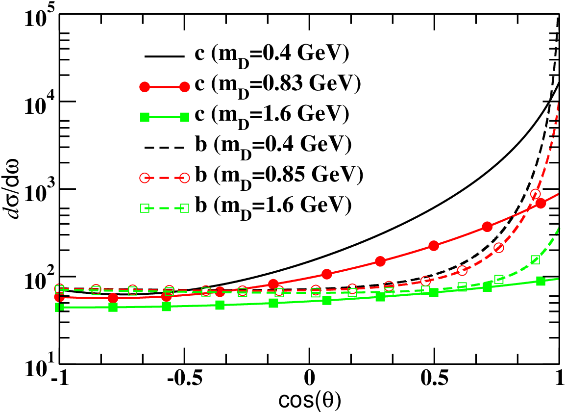

In Fig.2 we show the momentum transfer corresponding to different angular distributions or different values of Debye screening masses for both charm (solid lines) and bottom (dashed lines) quarks as a function of the HQ momentum when the bulk medium is at a temperature . We have estimated the momentum transferred as a function of p using the Boltzmann approach. We evaluate the total momentum transferred for particles in each interval and divide it by the total number of collisions in such an interval. For an HQ momentum we see that one goes from a momentum transfer for the forward peaked scattering matrix corresponding to to a for the nearly isotropic cross section corresponding to . For bottom quarks, due to their larger mass corresponding to , the change is less pronounced and for nearly isotropic cross sections is at most about 0.8 GeV.

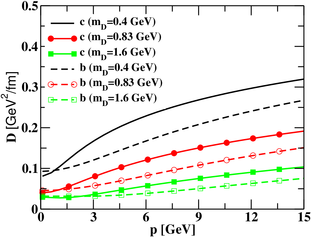
Starting from the same scattering matrix, , we have evaluated the Drag A(p) and Diffusion constant B(p) that enter into Langevin equation, see Eq. 6. The results are shown in Fig.s 3 and 4 for both charm (solid lines) and bottom (dashed lines) quarks at a temperature MeV for different values of that give rise to different values of drag and diffusion coefficients. The coupling has been kept fixed for all the cases. In order to have a similar within the typical time scale of uRHIC , the has been multiplied by a k factor. This has been chosen to be for , for and for [46]. For the same factor is of course rescaled also the cross section used to determine the evolution within the Boltzmann equation. Once the coefficients are rescaled by , they become approximately equal at GeV for the different . However the effect discussed does not depend on such factor that has been included only to set similar time scales for the evolution of the spectra reaching similar to that observed in HIC at momenta of about . However there is no necessity to set them exactly equal because we are interested only in comparing the Fokker-Planck and Boltzmann evolution starting from the same kernel (same ) given by the scattering matrix.
IV Numerical results: comparing the Boltzmann and Langevin evolution
We now discuss the evolution of momentum distributions of charm and bottom quarks interacting with a bulk medium at with scattering processes determined by the scattering matrices discussed in the previous section. The initial distribution of heavy quarks are taken from Ref. [4] and given by with , and for charm and bottom quarks respectively. The above function gives a reasonable description of D and B meson spectra in the p-p collision at highest RHIC energy. For the sake of comparison, we solve both the Langevin equation and the Boltzmann equation as described in Section II and III in a box with a volume . Our purpose is to compare the time evolution starting from the same initial momentum distribution for the both cases. The differential cross section , main ingredient of the Boltzmann equation, and the drag and diffusion coefficients, key ingredient of the Langevin equation, both originated from the same scattering matrix.
We have plotted the results as a ratio between Langevin to Boltzmann at different times to quantify how much the ratio deviates from 1. We started the simulation at fm/c which of course corresponds to a ratio of 1 as we start the simulation with the same initial momentum distribution for both Langevin and Boltzmann equations. So any deviation from 1 would reflect how much the Langevin differ from the Boltzmann evolution.


In Fig 5 the ratio of Langevin to Boltzmann spectra for the charm quark with GeV has been displayed as a function of momentum at different time. From Fig 5 it is observed that for fm the deviation of Langevin from Boltzmann is around and for fm the deviation is around a at GeV, which suggests the Langevin approach overestimates the average energy loss considerably due to the approximation it involves.
We remind that time scales of fm/c can be roughly taken as those corresponding to the typical lifetime of a QGP in uRHIC’s. This is why we are displaying and discussing the results around such a time. The same ratio is depicted in Fig 6 for GeV which is only a way to simulate a quite forward peaked scattering. The results presented in Fig 6 shown that Langevin dynamics deviates from the Boltzmann by about a at fm and . The reduced deviation between Langevin and Boltzmann for GeV can be expected knowing that for such a case where the scattering are more forward peaked and the average transfer momentum is about a factor of two smaller with respect to the case GeV, as shown in Fig.2. On the contrary, when we consider a larger screening mass, GeV to simulate a nearly isotropic scattering, the transferred momentum is about a factor of three larger and we see that the ratio of Langevin to Boltzmann spectra in Fig 7 at different time can lead to differences as large as a factor at t=4 fm/c. It is however important to report that for this last case the results depend on the procedure chosen to determine the Drag A(p) and Diffusion coefficients D(p). The results shown in Fig.7 is for the case where both coefficients are evaluated directly from the . However just for this case if one calculates the diffusion coefficient from the scattering matrix and the drag one from the constraint of the fluctuation dissipation theorem (FDT) the result are significantly modified. In particular the LV/BM ratio will evolve quite slowly and the ratio reaches value about at t=4 fm/c. Such ambiguity in determining the drag and diffusion coefficient is much less relevant for the case of smaller , however it essentially means that for nearly isotropic scatterings associated to large momentum transfer the dynamics of the scattering cannot be really encased simply into a shift of the average momenta with a Gaussian diffusion round the mean. This manifests into a stronger breaking of the FDT when both drag and diffusion are evaluated from .

We now move to the calculation for bottom quarks. In Fig. 8 the results for bottom quark are displayed for GeV. It is observed that the ratio stays practically around one for bottom quark for all the time evolution considered in the manuscript. The results for the other two values of are quite similar Therefore, for bottom quark the Langevin approach is really a good approximation of the Boltzmann equation independently of the angular dependence of the scatterings, at most a difference is observed for GeV. On the other hand, as already mentioned due to the large bottom mass an approximation of the dynamics to a Brownian motion appears always appropriate. We notice that this is determined by the ratio of the mass and the temperature that determines the average momentum of the particles colliding with heavy quarks (). For the bottom quark while for charm quark for the temperature we are considering.


IV.1 Momentum spread of heavy quarks
To further investigate the differences between the heavy quark dynamics implied by a Langevin and a Boltzmann approach, we study the heavy quark momentum evolution considering the initial charm and bottom quark distribution as a delta distribution at GeV for the case with GeV. The momentum evolution of the charm quarks is displayed in Fig. 9 within the Langevin dynamics. It is observed that the distributions are Gaussian as expected by construction. As known the Langevin dynamics consists of a shift of the average momenta with a fluctuation around such a value that includes also the possibility to gain energy for the HQ as we see from the tail of the momentum distribution that overshoots the initial momentum at , blue dashed line in Fig.9.


In Fig. 10 we present the momentum distribution for charm quark within the Boltzmann
equation. In this case the evolution of the charm quarks momentum does not have a Gaussian shape
and already at has a very different spread in momentum with a larger contribution from processes
where the charm quark can gain energy and a long tail at low momenta corresponding to some probability
to lose a quite large amount of energy
and in general a global shape that is not a at all of Gaussian form.
This essentially indicates that for a particle with as it is for the charm
quark at a temperature
, the evolution is not of Brownian type.
For the bottom quarks, shown in Fig. 11 and Fig. 12 , the momentum evolution gives
a much better agreement between the Boltzmann
and the Langevin evolution because . To further
support this argument we have also studied the evolution of charm in a medium at
as shown in Fig. 13, where ,
and in this case we have also found for the charm quark a momentum distribution similar
to the bottom one shown in Fig. 12.
We notice that in Fig. 13 we have plotted the momentum
distribution at larger time steps with respect to the figures at MeV.
This is because the
drag coefficient at MeV is about a factor three smaller than the case at MeV.
Therefore, we have chosen to plot
the distribution at time steps such that is almost the same as in the
previous Fig. 9 and 10.
Finally, we notice that even in the bottom case at () the evolution of the global spectra are practically identical between the Langevin and Boltzmann dynamics, see Fig.8, the detail of the energy loss of a single bottom quark remains still significantly different. The momentum distribution is reminiscent of a Gaussian distribution showing clearly a peak around the average momentum, but still it has an asymmetric distribution with a long tail towards lower momenta.
It would be interesting to study observables that are sensitive to such details of the HQ dynamics. A first candidate could be the and/or correlation [48] that should be quite different in a Langevin dynamics with respect to the Boltzmann one since the momentum evolution of a single quark is so different, in particular for charm quarks. For the charm quark the very different change in momenta could determine also a quite different dynamics for the suppression of charmonium in the medium.
IV.2 Time Evolution of the Nuclear Modification factor
One of the key observable, investigated at RHIC and LHC energies, is the depletion of high particles (D and B mesons or single ) produced in Nucleus-Nucleus collisions with respect to those produced in proton- proton collisions expressed through the nuclear suppression factor . Therefore, we look at the evolution of the spectra in terms of the for charm quarks evolving according to the LV and BM transport equations. We calculate the nuclear suppression factor, , using our initial and as final the charm quark distribution as .


The nuclear suppression factor, , has been displayed in Fig 14 as a function of momentum from both Langevin and Boltzmann side at different time for GeV. From Fig 14 it is observed that the time evolution of the nuclear suppression factor differs substantially from Langevin to Boltzmann at a given time. Similar trends are seen also at GeV but with a much smaller deviation of the order of while at GeV the deviation in the time evolution are even larger, we will discuss them more quantitatively before closing this Section.
The Diffusion coefficient has a significant importance for the phenomenological study. Hence, it is more meaningful from a phenomenological point of view to evaluate how much we need to change the diffusion coefficient/interaction from Langevin side to reproduce the same nuclear suppression factor as for the Boltzmann equation. We find that (Fig. 15) a reduction of the diffusion coefficients is needed for the Langevin equation by (or we need only in the LV ) to get a similar nuclear suppression factor as of the Boltzmann equation at time fm/c which is the typical lifetime of the system produced at RHIC. We do not display the experimental data because we are simply studying the evolution of in a box at fixed . Still one gets an idea of the differences that may be found with a realistic expanding QGP background . It is interesting to note that even if we put the emphasis on the different dynamical evolution between BM and LV, at the end one can obtain an identical (almost) in all the range just by reducing the interaction of about . It may be mentioned here that in the present calculation of , both the drag and diffusion coefficients are taken from pQCD calculation to capture the actual dynamical evolution. It is found that if we use the diffusion coefficient from pQCD and drag coefficient in accordance with Einstein relation, the differ about at GeV and bit less at low momentum for fm/c with respect to the case when both the drag and diffusion coefficients are taken from pQCD, as we do in this paper.
In Fig 16 we plotted as a function of momentum from for GeV. For this case the Langevin results differ drastically from Boltzmann as the momentum transfer is very large, but still one can compensate the difference between Langevin and Boltzmann, having exactly the same by reducing by about a of the diffusion coefficient for the LV evolution. However, as mentioned in the previous subsection for GeV there can be significant dependency whether both A and D coefficients are taken from the pQCD calculations or the fluctuation-dissipation theorem is implemented. We have checked that this can reduce or enhance the differences between the LV and BM dynamics. However, our main aim here is simply to show that even if the underlying dynamics of the charm quark can be quite different between the LV and the BM transport approaches at the level of the , one can anyway mimic the same result mocking the differences in the dynamical evolution by modifying the interaction by an amount that can go from about a up to about a depending on the angular dependence of the scatterings that entails the strength of the transferred momentum. We have not shown results for the bottom case because, as discussed in the first part of this section we do not observe significant differences in the time evolution of the spectra between the LV and BM descriptions.
V Comparison with the Experimental observables
In order to study the impact of the results presented in the previous sections on the phenomenology of heavy-ion collisions, we present here a first comparison between the results obtained within the Boltzmann and the Langevin approach with the experimental data. We have performed simulation of collisions at AGeV for the minimum bias using a 3+1D transport approach [40, 41, 42]. The initial conditions for the bulk in the -space are given by the standard Glauber condition, while in the -space we use a Boltzmann-Juttner distribution function up to a transverse momentum GeV and at larger momenta mini-jet distributions as calculated by pQCD at NLO order [25]. The initial maximum temperature at the center of the fireball is MeV and the initial time for the simulations is fm/c (corresponding to the criteria). The distributions in p-space for the HQ are the same as described in the previous section and in r-space they are distributed according to . Of course the same bulk that we get within the Boltzmann equation is used for both the Langevin and Boltzmann approaches.


We convolute the solution with the fragmentation functions of the heavy quarks at the transition temperature to obtain the momentum distribution of the heavy mesons (B and D). The Peterson function has been used for heavy quark fragmentation:
| (11) |
for charm quark . For bottom quark .
We calculate the nuclear suppression factor, , using our initial and final heavy meson (D or B) distribution as . The anisotropic momentum distribution induced by the spatial anisotropy of the bulk can be calculated by means of the quantity :
| (12) |
measuring the momentum space anisotropy.
As we mentioned earlier, it is a challenge for all the models to describe the and simultaneously for the same set of inputs. In Fig. 17 we have shown the as a function of . In the present study, we try to reproduce the same (almost) from both the LV and BM side (as we did in Fig. 15 and Fig. 16 ) and study the corresponding . To obtain a very similar in LV and BM for the expanding medium, one needs to reduce the interaction from the LV side similarly to the static case.
In Fig. 18 we have plotted as a function of calculated from both the LV and BM dynamics. Our main conclusion is that even if the is very similar in both cases, the full BM dynamics generates a sizable larger (about ) toward a better agreement with the experimental data at RHIC [20] energy. The present calculation is performed at =1.6 GeV (isotropic cross section) which allows to simulate the case of nearly isotropic cross section estimating roughly the maximum effect that the BM dynamics can have with respect to the LV dynamics for experimental observables. In BM case, we are getting a larger , most likely due to the large spreading of momentum, see Fig. 10, implying that the charm quark mixes up with the bulk participating more effectively to the dynamics of the expanding medium. The effect on for the same is still significant, about , for (similarly for ), while it becomes negligible for (or more generally for ). We notice that with the isotropic cross section one may nearly reproduce the and simultaneously within the BM approach.
VI Summary and conclusions
We present a study of the implications of the approximations involved in the Langevin equation by mean of a direct comparison with the full collisional integral (no small momentum transferred approximation) within the framework of the Boltzmann transport equation. We consider a box where the bulk is in equilibrium at T=0.2-0.4 GeV. For the realistic initial momentum distribution, we found that the Langevin approach is a very good approximation for bottom quark whereas for charm quark Langevin approach can deviate significantly from the full Boltzmann transport equation depending on different values of . The difference for GeV is about a at intermediate momentum for a time evolution of 5-6 fm/c typical of the QGP created in heavy-ion collisions . The deviation goes down to about a for the same range of momentum and time for the case GeV. For GeV the difference is about a at intermediate momentum, but the exact amount depends on the way the fluctuations-dissipation theorem is implemented. Hence, the effect for charm quarks can be significantly larger or smaller depending on the values of Debye screening mass and/or on the angular dependence of the collisions. However we notice that one can get a very similar suppression factor from both the approaches just reducing the diffusion coefficient of the Langevin approach by around for GeV. For GeV such reduction should be about a .
The present uncertainties on the charm transport coefficients is indeed even larger. If such an ambiguity on the value of the drag or diffusion coefficient is discarded looking only at one can conclude the Langevin dynamics supplies a sufficiently good approximation of the Boltzmann collision integral, even if we warn that the detail of the single quark energy loss spread could be quite different in the two cases. In fact, we have also performed the comparison for the case considering the initial distribution as a delta peaked at GeV. We found that both the charm and bottom quarks are Gaussian like distribution within the Langevin dynamics while the distribution obtained, for charm quarks, within the Boltzmann equation is a quite different one revealing the fact that Langevin dynamics of the charm quark may not work in a hot QCD medium. For the bottom quarks the approximation looks reasonable.
More specifically, we have found that the underlying dynamics of the single heavy quarks are indeed quite different between the Boltzmann and the Langevin approach. In practice the dynamical evolution of a single charm does not appear to be simply a shift in momentum with a Gaussian fluctuations around it. Indeed one can say that this can be expected considering that for charm quarks for a typical temperature at RHIC and LHC energies, which makes the assumption of Brownian motion questionable. On the contrary, for bottom quarks we do find that the dynamical evolution is approximately that of Brownian motion even if the fluctuation around the average momentum still appear to deviate from a Gaussian shape and are more reminiscent of the binomial distribution. These results can have significant effects on the heavy ion phenomenology at RHIC and LHC energies.
Finally we presented a first comparison between LV and BM approach for a realistic fireball evolution as created in ultra-relativistic heavy-ion collisions at RHIC energy. We have found that with the isotropic cross section the BM approach gets close to reproducing the and simultaneously while the LV dynamics generate a smaller elliptic flow in correspondence to the same .
Acknowledgments
We acknowledge the support by the ERC StG under the QGPDyn Grant n. 259684. We acknowledge to T. Bhattacharyya for reading the manuscript.
VII Appendix
In this appendix we quote the invariant amplitude for the elastic processes used for evaluating the drag and diffusion coefficients of charm and bottom quarks considering the bulk consists of only gluons.
The invariant amplitude, for the process is given by:
| (13) |
where s,t and u are the Mandelstam variables and is the mass of the heavy quark. Integrating the invariant amplitude over the variable t, between the integration limits
| (14) |
we get the total cross section
| (15) |
that we need to evaluate the collision integral in eq. 1.
References
- [1] E. V. Shuryak, Nucl. Phys. A 750 (2005) 64
- [2] B. V. Jacak and B. Muller, Science 337, 310 (2012).
- [3] R.Rapp and H van Hees, R. C. Hwa, X. N. Wang (Ed.) Quark Gluon Plasma 4, 2010, World Scientific, 111 [arXiv:0903.1096 [hep-ph]]
- [4] M. Cacciari, P. Nason and R. Vogt, Phys. Rev. Lett. 95 (2005) 122001
- [5] M. Cacciari, S. Frixione, N. Houdeau, M. L. Mangano, P. Nason and G. Ridolfi, JHEP 1210 (2012) 137
- [6] B. Svetitsky, Phys. Rev. D 37, 2484 (1988)
- [7] M.G. Mustafa, D. Pal and D. K. Srivastava, Phys. Rev. C 57, 889 (1998)
- [8] G. D. Moore, D Teaney, Phys. Rev. C 71, 064904 (2005)
- [9] H. van Hees, V. Greco and R. Rapp, Phys. Rev. C 73, 034913 (2006)
- [10] S. Cao, S. A. Bass, Phys. Rev. C 84, 064902 (2011)
- [11] M. Djordjevic, M. Gyulassy, R. Vogt and S. Wicks, Phys. Lett. B 632 (2006) 81
- [12] N. Armesto, M. Cacciari, A. Dainese, C. A. Salgado and U. A. Wiedemann, Phys. Lett. B 637 (2006) 362
- [13] S. Batsouli, S. Kelly, M. Gyulassy and J. L. Nagle, Phys. Lett. B 557 (2003) 26
- [14] V. Greco, C. M. Ko and R. Rapp, Phys. Lett. B 595 (2004) 202
- [15] H. Van Hees, M. Mannarelli, V. Greco and R. Rapp, Phys. Rev. Lett. 100,192301 (2008)
- [16] P. B. Gossiaux, J. Aichelin, Phys. Rev. C 78 014904 (2008); P.B. Gossiaux, J. Aichelin, T. Gousset and V. Guiho, J. Phys. G 37, 094019 (2010)
- [17] A. Adare et al. (PHENIX Collaboration), Phys. Rev. Lett. 98, 172301 (2007).
- [18] B. I. Abeleb et al. (STAR Collaboration), Phys. Rev. Lett. 98, 192301 (2007).
- [19] S. S. Adler et al. (PHENIX Collaboration), Phys. Rev. Lett. 96, 032301 (2006).
- [20] A. Adare et al. (PHENIX Collaboration), Phys. Rev. C 84, 044905 (2011)
- [21] B. Abelev et al.,(ALICE Collaboration) JHEP 1209 (2012) 112
- [22] P. B. Gossiaux et al., arXiv:1102.1114 [hep-ph]
- [23] P. B. Gossiaux, J. Aichelin, M. Bluhm, T. Gousset, M. Nahrgang, S. Vogel and K. Werner, PoS QNP 2012 (2012) 160 [arXiv:1207.5445 [hep-ph]]
- [24] C. M. Ko and W. Liu, Nucl. Phys. A 783, 23c (2007).
- [25] V. Greco, C. M. Ko and P. Levai, Phys. Rev. Lett. 90 (2003) 202302; V. Greco, C. M. Ko and P. Levai, Phys. Rev. C 68 (2003) 034904
- [26] Y. Akamatsu, T. Hatsuda and T. Hirano, Phys. Rev. C 79, 054907 (2009)
- [27] S. K Das, J. Alam and P. Mohanty, Phys. Rev. C 82, 014908 (2010); S. Majumdar, T. Bhattacharyya, J. Alam and S. K. Das, Phys. Rev. C 84 , 044901 (2012)
- [28] W. M. Alberico et al., Eur. Phys. J. C, 71 1666 (2011); W. M. Alberico et al., Eur. Phys. J. C 73 2481 (2013)
- [29] C. Young , B. Schenke , S. Jeon and C. Gale, Phys. Rev. C 86, 034905 (2012)
- [30] M. Younus, C. E. Coleman-Smith, S. A. Bass and D. K. Srivastava, arXiv:1309.1276 [nucl-th].
- [31] B. Zhang, L. -W. Chen and C. -M. Ko, Phys. Rev. C 72 (2005) 024906
- [32] D. Molnar, Eur. Phys. J. C 49 (2007) 181
- [33] S. K. Das, F. Scardina, S. Plumari and V. Greco, arXiv:1309.7930 [nucl-th]
- [34] T. Lang, H. van Hees, J. Steinheimer and M. Bleicher, arXiv:1208.1643 [hep-ph]
- [35] S. Cao, G-Y. Qin, S. A. Bass and B. Müller, Nucl. Phys. A 904, 653c (2013)
- [36] Hao-jie Xu, Xin Dong, Li-juan Ruan, Qun Wang, Zhang-bu Xu, and Yi-fei Zhang, arXiv:1305:7302
- [37] M. He, R. J. Fries and R. Rapp, Phys. Rev. Lett. 110, 112301 (2013)
- [38] D. B. Walton and J. Rafelski, Phys. Rev. Lett. 84, 31 (2002)
- [39] S. Majumdar, T Bhattacharyya and J. Alam, Phys. Rev. D 89, 014002 (2014)
- [40] G. Ferini, M. Colonna , M. Di Toro and V. Greco, Phys. Lett. B, 670,325 (2009); V. Greco, M. Colonna,M. Di Toro and G. Ferini, Progr. Part. Nucl. Phys. 62, 562 (2009)
- [41] M. Ruggieri, F. Scardina, S. Plumari and V. Greco, Phys. Lett. B 727 (2013) 177
- [42] F. Scardina, M. Colonna, S. Plumari and V. Greco, Phys. Lett. B 724 (2013) 296
- [43] Z. Xu and C. Greiner, Phys. Rev. C 71, 064901 (2005)
- [44] A. Meistrenko, A. Peshier, J. Uphoff and C. Greiner, Nucl. Phys. A 901 (2013) 51
- [45] A. Lang et al., Jour. of Comp. Phys. 106, 391 (1993)
- [46] J. Uphoff, O. Fochler, Z. Xu and C. Greiner, Phys. Rev. C, 84 024908 (2011)
- [47] J. Uphoff, O. Fochler, Z. Xu and C. Greiner, Phys. Lett. B 717 (2012) 430
- [48] X. Zhu and N. Xu and P. Zhuang, Phys. Rev. Lett. 100, 152301 (2008)