跳到论文正文
W Papers独立论文阅读器 arXiv:1312.6818 论文正文 计算阅读时间 · 0%
引用这篇论文根据当前论文元数据生成,正式投稿前建议核对。


License: arXiv.org perpetual non-exclusive license
arXiv:1312.6818v2 [hep-ex] 12 Mar 2014

Test of CPT\mathrm{CPT} and Lorentz symmetry in entangled neutral kaons with the KLOE experiment

Journal: Physics Letter B
The KLOE-2 Collaboration    D. Babusci Address: Laboratori Nazionali di Frascati dell’INFN, Frascati, Italy.    I. Balwierz-Pytko Address: Institute of Physics, Jagiellonian University, Cracow, Poland.    G. Bencivenni Address: Laboratori Nazionali di Frascati dell’INFN, Frascati, Italy.    C. Bloise Address: Laboratori Nazionali di Frascati dell’INFN, Frascati, Italy.    F. Bossi Address: Laboratori Nazionali di Frascati dell’INFN, Frascati, Italy.    P. Branchini Address: INFN Sezione di Roma Tre, Roma, Italy.    A. Budano Address: Dipartimento di Matematica e Fisica dell’Università “Roma Tre”, Roma, Italy. Address: INFN Sezione di Roma Tre, Roma, Italy.    L. Caldeira Balkeståhl Address: Department of Physics and Astronomy, Uppsala University, Uppsala, Sweden.    G. Capon Address: Laboratori Nazionali di Frascati dell’INFN, Frascati, Italy.    F. Ceradini Address: Dipartimento di Matematica e Fisica dell’Università “Roma Tre”, Roma, Italy. Address: INFN Sezione di Roma Tre, Roma, Italy.    P. Ciambrone Address: Laboratori Nazionali di Frascati dell’INFN, Frascati, Italy.    F. Curciarello Address: INFN Sezione di Catania, Catania, Italy. Address: Dipartimento di Fisica e Scienze della Terra dell’Università di Messina, Messina, Italy.    E. Czerwiński Address: Institute of Physics, Jagiellonian University, Cracow, Poland.    E. Danè Address: Laboratori Nazionali di Frascati dell’INFN, Frascati, Italy.    V. De Leo Address: INFN Sezione di Catania, Catania, Italy. Address: Dipartimento di Fisica e Scienze della Terra dell’Università di Messina, Messina, Italy.    E. De Lucia Address: Laboratori Nazionali di Frascati dell’INFN, Frascati, Italy.    G. De Robertis Address: INFN Sezione di Bari, Bari, Italy.    A. De Santis Email: antonio.desantis@roma1.infn.it URL: http://www.lnf.infn.it/ãdesanti Corresponding author: Corresponding author Address: Dipartimento di Fisica dell’Università “Sapienza”, Roma, Italy. Address: INFN Sezione di Roma, Roma, Italy.    P. De Simone Address: Laboratori Nazionali di Frascati dell’INFN, Frascati, Italy.    A. Di Cicco Address: Dipartimento di Matematica e Fisica dell’Università “Roma Tre”, Roma, Italy. Address: INFN Sezione di Roma Tre, Roma, Italy.    A. Di Domenico Address: Dipartimento di Fisica dell’Università “Sapienza”, Roma, Italy. Address: INFN Sezione di Roma, Roma, Italy.    C. Di Donato Address: Dipartimento di Fisica dell’Università “Federico II”, Napoli, Italy. Address: INFN Sezione di Napoli, Napoli, Italy.    R. Di Salvo Address: INFN Sezione di Roma Tor Vergata, Roma, Italy.    D. Domenici Address: Laboratori Nazionali di Frascati dell’INFN, Frascati, Italy.    O. Erriquez Address: Dipartimento di Fisica dell’Università di Bari, Bari, Italy. Address: INFN Sezione di Bari, Bari, Italy.    G. Fanizzi Address: Dipartimento di Fisica dell’Università di Bari, Bari, Italy. Address: INFN Sezione di Bari, Bari, Italy.    A. Fantini Address: Dipartimento di Fisica dell’Università “Tor Vergata”, Roma, Italy. Address: INFN Sezione di Roma Tor Vergata, Roma, Italy.    G. Felici Address: Laboratori Nazionali di Frascati dell’INFN, Frascati, Italy.    S. Fiore Address: Dipartimento di Fisica dell’Università “Sapienza”, Roma, Italy. Address: INFN Sezione di Roma, Roma, Italy.    P. Franzini Address: Dipartimento di Fisica dell’Università “Sapienza”, Roma, Italy. Address: INFN Sezione di Roma, Roma, Italy.    A. Gajos Address: Institute of Physics, Jagiellonian University, Cracow, Poland.    P. Gauzzi Address: Dipartimento di Fisica dell’Università “Sapienza”, Roma, Italy. Address: INFN Sezione di Roma, Roma, Italy.    G. Giardina Address: INFN Sezione di Catania, Catania, Italy. Address: Dipartimento di Fisica e Scienze della Terra dell’Università di Messina, Messina, Italy.    S. Giovannella Address: Laboratori Nazionali di Frascati dell’INFN, Frascati, Italy.    E. Graziani Address: INFN Sezione di Roma Tre, Roma, Italy.    F. Happacher Address: Laboratori Nazionali di Frascati dell’INFN, Frascati, Italy.    L. Heijkenskjöld Address: Department of Physics and Astronomy, Uppsala University, Uppsala, Sweden.    B. Höistad Address: Department of Physics and Astronomy, Uppsala University, Uppsala, Sweden.    M. Jacewicz Address: Department of Physics and Astronomy, Uppsala University, Uppsala, Sweden.    T. Johansson Address: Department of Physics and Astronomy, Uppsala University, Uppsala, Sweden.    K. Kacprzak Address: Institute of Physics, Jagiellonian University, Cracow, Poland.    D. Kamińska Address: Institute of Physics, Jagiellonian University, Cracow, Poland.    A. Kupsc Address: Department of Physics and Astronomy, Uppsala University, Uppsala, Sweden.    J. Lee-Franzini Address: Laboratori Nazionali di Frascati dell’INFN, Frascati, Italy. Address: Physics Department, State University of New York at Stony Brook, USA.    F. Loddo Address: INFN Sezione di Bari, Bari, Italy.    S. Loffredo Address: Dipartimento di Matematica e Fisica dell’Università “Roma Tre”, Roma, Italy. Address: INFN Sezione di Roma Tre, Roma, Italy.    G. Mandaglio Address: Centro Siciliano di Fisica Nucleare e Struttura della Materia, Catania, Italy. Address: INFN Sezione di Catania, Catania, Italy. Address: Dipartimento di Fisica e Scienze della Terra dell’Università di Messina, Messina, Italy.    M. Martemianov Address: Institute for Theoretical and Experimental Physics (ITEP), Moscow, Russia.    M. Martini Address: Laboratori Nazionali di Frascati dell’INFN, Frascati, Italy. Address: Dipartimento di Scienze e Tecnologie applicate, Università “Guglielmo Marconi", Roma, Italy.    M. Mascolo Address: Dipartimento di Fisica dell’Università “Tor Vergata”, Roma, Italy. Address: INFN Sezione di Roma Tor Vergata, Roma, Italy.    R. Messi Address: Dipartimento di Fisica dell’Università “Tor Vergata”, Roma, Italy. Address: INFN Sezione di Roma Tor Vergata, Roma, Italy.    S. Miscetti Address: Laboratori Nazionali di Frascati dell’INFN, Frascati, Italy.    G. Morello Address: Laboratori Nazionali di Frascati dell’INFN, Frascati, Italy.    D. Moricciani Address: INFN Sezione di Roma Tor Vergata, Roma, Italy.    P. Moskal Address: Institute of Physics, Jagiellonian University, Cracow, Poland.    F. Nguyen Address: INFN Sezione di Roma Tre, Roma, Italy. Address: Present Address: Laboratório de Instrumentação e Física Experimental de Partículas, Lisbon, Portugal.    A. Palladino Address: Laboratori Nazionali di Frascati dell’INFN, Frascati, Italy.    A. Passeri Address: INFN Sezione di Roma Tre, Roma, Italy.    V. Patera Address: Laboratori Nazionali di Frascati dell’INFN, Frascati, Italy. Address: Dipartimento di Scienze di Base ed Applicate per l’Ingegneria dell’Università “Sapienza”, Roma, Italy.    I. Prado Longhi Address: Dipartimento di Matematica e Fisica dell’Università “Roma Tre”, Roma, Italy. Address: INFN Sezione di Roma Tre, Roma, Italy.    A. Ranieri Address: INFN Sezione di Bari, Bari, Italy.    P. Santangelo Address: Laboratori Nazionali di Frascati dell’INFN, Frascati, Italy.    I. Sarra Address: Laboratori Nazionali di Frascati dell’INFN, Frascati, Italy.    M. Schioppa Address: Dipartimento di Fisica dell’Università della Calabria, Cosenza, Italy. Address: INFN Gruppo collegato di Cosenza, Cosenza, Italy.    B. Sciascia Address: Laboratori Nazionali di Frascati dell’INFN, Frascati, Italy.    M. Silarski Address: Institute of Physics, Jagiellonian University, Cracow, Poland.    C. Taccini Address: Dipartimento di Matematica e Fisica dell’Università “Roma Tre”, Roma, Italy. Address: INFN Sezione di Roma Tre, Roma, Italy.    L. Tortora Address: INFN Sezione di Roma Tre, Roma, Italy.    G. Venanzoni Address: Laboratori Nazionali di Frascati dell’INFN, Frascati, Italy.    W. Wiślicki Address: National Centre for Nuclear Research, Warsaw, Poland.    M. Wolke Address: Department of Physics and Astronomy, Uppsala University, Uppsala, Sweden.    J. Zdebik Address: Institute of Physics, Jagiellonian University, Cracow, Poland.
Abstract

Neutral kaon pairs produced in ϕ\upphi decays in anti-symmetric entangled state can be exploited to search for violation of CPT\mathrm{CPT} symmetry and Lorentz invariance. We present an analysis of the CP\mathrm{CP}-violating process ϕ\upphi→\rightarrowKS\mathrm{K}_{\mathrm{S}}KL\mathrm{K}_{\mathrm{L}}→\rightarrowπ+\uppi^{+}π−\uppi^{-}π+\uppi^{+}π−\uppi^{-} based on 1.7 fb−1\mathrm{fb}^{-1} of data collected by the KLOE experiment at the Frascati ϕ\upphi–factory DAΦ\UpphiNE. The data are used to perform a measurement of the CPT\mathrm{CPT}-violating parameters Δ​aμ\Delta a_{\mu} for neutral kaons in the context of the Standard Model Extension framework. The parameters measured in the reference frame of the fixed stars are:
Δ​a0=(−6.0±7.7s​t​a​t±3.1s​y​s​t)×10−18​GeV\Delta a_{0}=(-6.0\pm 7.7_{stat}\pm 3.1_{syst})\times 10^{-18}\,\,\mathrm{GeV}
Δ​aX=(   0.9±1.5s​t​a​t±0.6s​y​s​t)×10−18​GeV\Delta a_{\mathrm{X}}=(\,\,\,0.9\pm 1.5_{stat}\pm 0.6_{syst})\times 10^{-18}\,\,\mathrm{GeV}
Δ​aY=(−2.0±1.5s​t​a​t±0.5s​y​s​t)×10−18​GeV\Delta a_{\mathrm{Y}}=(-2.0\pm 1.5_{stat}\pm 0.5_{syst})\times 10^{-18}\,\,\mathrm{GeV}
Δ​aZ=(   3.1±1.7s​t​a​t±0.5s​y​s​t)×10−18​GeV\Delta a_{\mathrm{Z}}=(\,\,\,3.1\pm 1.7_{stat}\pm 0.5_{syst})\times 10^{-18}\,\,\mathrm{GeV}
These are presently the most precise measurements in the quark sector of the Standard Model Extension.

Keywords: 
CPT\mathrm{CPT} symmetry, Lorentz symmetry, neutral kaons, ϕ\upphi–factory.

1 Introduction

The CPT\mathrm{CPT} theorem [1] ensures invariance under the simultaneous transformation of charge conjugation (C\mathrm{C}), parity (P\mathrm{P}) and time reversal (T\mathrm{T}), in the context of local quantum field theories with Lorentz invariance and Hermiticity. On the other hand CPT\mathrm{CPT} violation in any unitary, local, point-particle quantum field theory entails Lorentz invariance violation, as proved in a theorem by Greenberg [2]. Even though Lorentz symmetry has been verified in many experiments, as also CPT\mathrm{CPT} invariance, it can be considered a sensitive probe for physics at the Planck scale, where natural mechanisms for such violations exist in quantum theories of gravity [3].

An attractive possibility to describe CPT\mathrm{CPT} and Lorentz violation effects in the low energy regime accessible to experiments consists of using an effective field theory, independent of the underlying mechanism generating CPT\mathrm{CPT} and Lorentz violation. This can be obtained by adding to the Standard Model action all possible scalar terms formed by contracting operators for simultaneous CPT\mathrm{CPT} and Lorentz violation with coefficients that control the size of the effects. The resulting effective field theory, the Standard Model Extension (SME)[4], appears to be compatible with the basic tenets of quantum field theory and retains the properties of gauge invariance and renormalizability. The SME is quite general and widely used in a broad class of experimental tests of CPT\mathrm{CPT} and Lorentz symmetry in several physics domains ranging from atomic physics to particle physics and to cosmology [5].

In the present Letter we present a test of CPT\mathrm{CPT} and Lorentz symmetry in the neutral kaon system within the SME framework. It has been performed by analyzing the ϕ\upphi→\rightarrowKS\mathrm{K}_{\mathrm{S}}KL\mathrm{K}_{\mathrm{L}}→\rightarrowπ+\uppi^{+}π−\uppi^{-} π+\uppi^{+}π−\uppi^{-} events collected by the KLOE experiment at the DAΦ\UpphiNE ϕ\upphi–factory.

The physical neutral kaon states are expressed in terms of the flavor states as |KS,L⟩∝(1+ϵS,L)​|K0⟩±(1−ϵS,L)​|K¯0⟩,|\mathrm{K}_{\mathrm{S,L}}\rangle\propto(1+\epsilon_{S,L})|\mathrm{K}^{0}\rangle\pm(1-\epsilon_{S,L})|{\bar{\mathrm{K}}}^{0}\rangle~, with ϵS,L=ϵK±δK\epsilon_{\mathrm{S,L}}=\epsilon_{\mathrm{K}}\pm\delta_{\mathrm{K}} being the CP\mathrm{CP} impurities (ϵK\epsilon_{\mathrm{K}} and δK\delta_{\mathrm{K}} are the usual T\mathrm{T} and CPT\mathrm{CPT} violation parameters). In SME CPT\mathrm{CPT} violation manifests to lowest order only in the mixing parameter δK\delta_{\mathrm{K}}, (i.e. vanishes at first order in the decay amplitudes), and exhibits a dependence on the 4-momentum of the kaon [6]:

δK≈isinϕSWei​ϕSWγK(Δa0−βK→⋅Δa→)/Δm,\delta_{\mathrm{K}}\approx i\sin\phi_{\mathrm{SW}}e^{i\phi_{\mathrm{SW}}}\gamma_{\mathrm{K}}(\Delta a_{0}-\vec{\beta_{\mathrm{K}}}\cdot\Delta{\vec{a}})/\Delta m\,, (1)

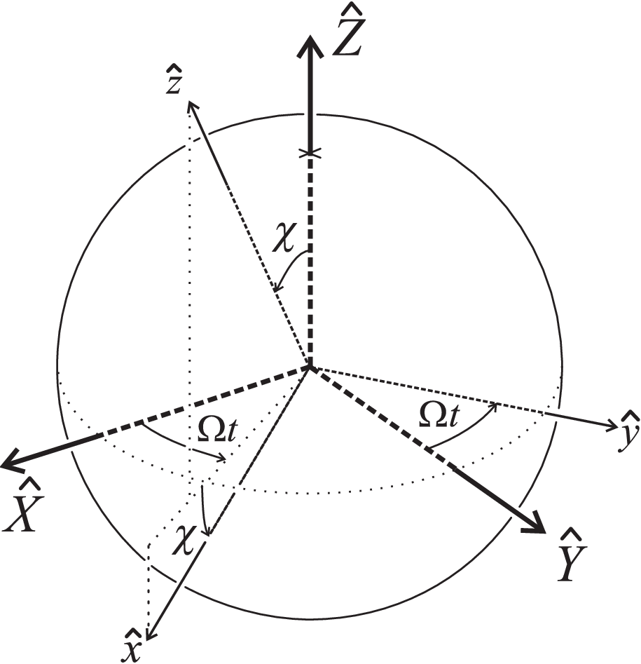
where γK\gamma_{\mathrm{K}} and βK→\vec{\beta_{\mathrm{K}}} are the kaon boost factor and velocity in the laboratory frame, ϕSW=arctan⁡(2​Δ​m/Δ​Γ)\phi_{\mathrm{SW}}=\arctan(2\Delta m/\Delta\Gamma) is the so-called superweak phase, Δ​m=mL−mS\Delta m=m_{\mathrm{L}}-m_{\mathrm{S}}, Δ​Γ=ΓS−ΓL\Delta\Gamma=\Gamma_{\mathrm{S}}-\Gamma_{\mathrm{L}} are the mass and width differences for the neutral kaon mass eigenstates, and Δ​aμ\Delta a_{\mu} are four CPT\mathrm{CPT} and Lorentz violating coefficients for the two valence quarks in the kaon11 1 Δ​aμ\Delta a_{\mu} parameters are associated with differences of terms in the SME of the form −aμq​q¯​γμ​q-a_{\mu}^{q}\bar{q}\gamma^{\mu}q, where qq is a quark field of a specific flavor [6].. The natural choice of the reference frame to observe these parameters is the reference frame defined by fixed stars. Following Ref. [6] and choosing a three-dimensional basis (X^,Y^,Z^\hat{X},\hat{Y},\hat{Z}) in this frame (with Z^\hat{Z} parallel to Earth’s rotation axis, X^\hat{X} expressed in terms of celestial equatorial coordinates with declination and right ascension 0∘0^{\circ}, while Y^\hat{Y} with declination 0∘0^{\circ} and right ascension 90∘90^{\circ}) and a basis (x^,y^,z^)(\hat{x},\hat{y},\hat{z}) for the laboratory frame according to Figure 1-left, (where z^\hat{z} is parallel to the beam axis with direction fixed by the positron beam and x^\hat{x} lies in the plane (z^,Z^)(\hat{z},\hat{Z})), the CPT\mathrm{CPT} violating parameter δK\delta_{\mathrm{K}} is expressed as:

δK​(p→,ts)\displaystyle\delta_{\mathrm{K}}(\vec{p},{t_{\mathrm{s}}}) =\displaystyle= isinϕSWei​ϕSWΔ​mγK[Δa0\displaystyle\frac{i\sin\phi_{\mathrm{SW}}e^{i\phi_{\mathrm{SW}}}}{\Delta m}\gamma_{\mathrm{K}}\Big[\Delta a_{0} (2)
+βK​Δ​aZ​(cos⁡ϑ​cos⁡χ−sin⁡ϑ​cos⁡φ​sin⁡χ)\displaystyle+\beta_{\mathrm{K}}{\Delta a_{\mathrm{Z}}}(\cos\vartheta\cos\chi-\sin\vartheta\cos\varphi\sin\chi)
−βK​Δ​aX​sin⁡ϑ​sin⁡φ​sin⁡Ω​ts\displaystyle-\beta_{\mathrm{K}}\Delta a_{\mathrm{X}}\sin\vartheta\sin\varphi\sin\Omega{t_{\mathrm{s}}}
+βK​Δ​aX​(cos⁡ϑ​sin⁡χ+sin⁡ϑ​cos⁡φ​cos⁡χ)​cos⁡Ω​ts\displaystyle+\beta_{\mathrm{K}}\Delta a_{X}(\cos\vartheta\sin\chi+\sin\vartheta\cos\varphi\cos\chi)\cos\Omega{t_{\mathrm{s}}}
+βK​Δ​aY​(cos⁡ϑ​sin⁡χ+sin⁡ϑ​cos⁡φ​cos⁡χ)​sin⁡Ω​ts\displaystyle+\beta_{\mathrm{K}}\Delta a_{\mathrm{Y}}(\cos\vartheta\sin\chi+\sin\vartheta\cos\varphi\cos\chi)\sin\Omega{t_{\mathrm{s}}}
+βKΔaYsinϑsinφcosΩts]\displaystyle+\beta_{\mathrm{K}}\Delta a_{\mathrm{Y}}\sin\vartheta\sin\varphi\cos\Omega{t_{\mathrm{s}}}\Big]

where p→\vec{p} is the kaon momentum, ts{t_{\mathrm{s}}} is the sidereal time, Ω\Omega is the Earth’s sidereal frequency, cos⁡χ=z^⋅Z^\cos\chi=\hat{z}\cdot\hat{Z}; ϑ\vartheta and φ\varphi are the conventional polar and azimuthal angles of the kaon momentum in the laboratory frame.
Refer to caption
Refer to caption
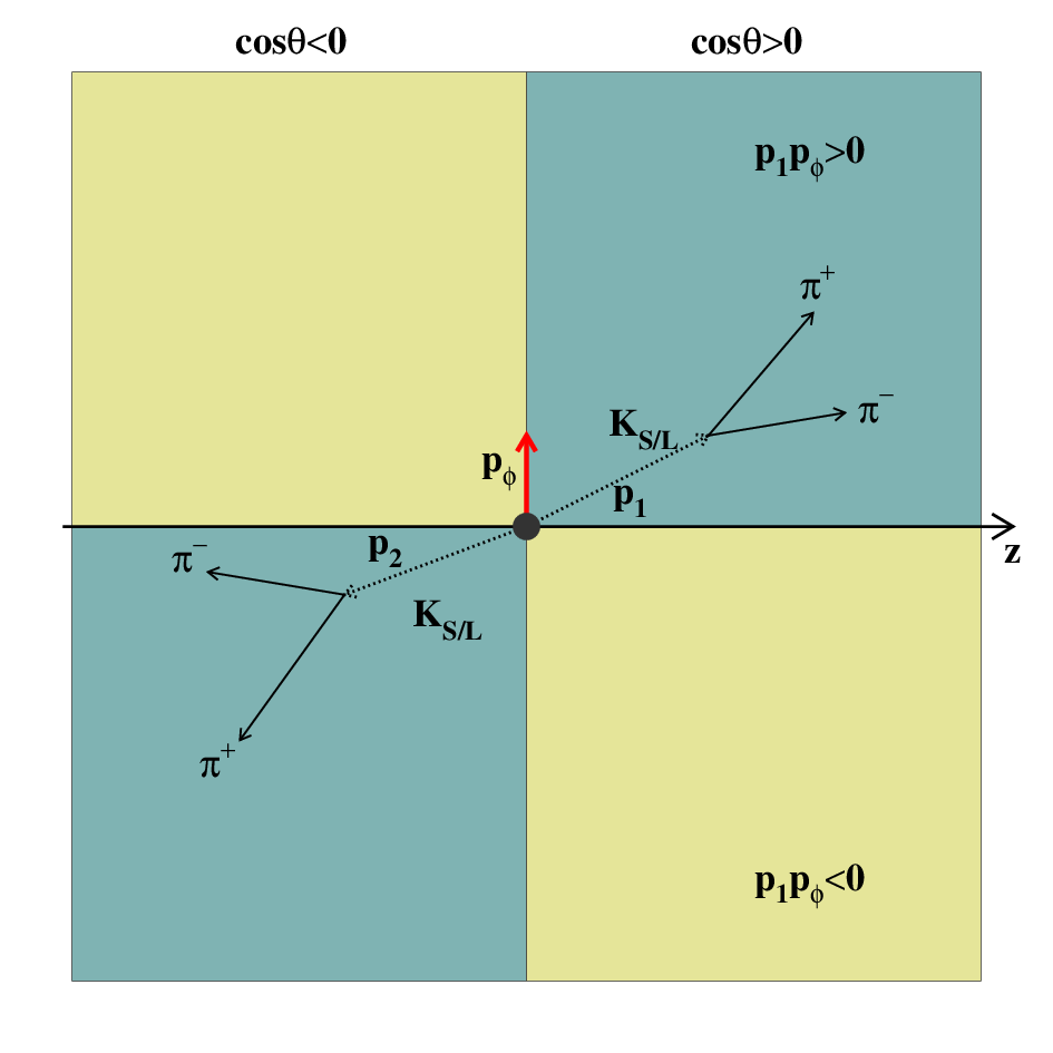
Figure 1: Left: Basis (x^,y^,z^)(\hat{x},\hat{y},\hat{z}) for the lab frame, and basis (X^,Y^,Z^)(\hat{X},\hat{Y},\hat{Z}) for the fixed stars frame. The laboratory frame precesses around the Earth’s rotation axis Z^\hat{Z} at the sidereal frequency Ω\Omega. The angle between Z^\hat{Z} and the positron beam direction z^\hat{z} defined in the laboratory frame of KLOE is χ≃113∘\chi\simeq 113^{\circ} (picture taken from Ref. [6]). Right: Sketch of the quadrant subdivisions as seen from a top view of the KLOE detector; p→ϕ{\vec{p}}_{\upphi} is lying in the horizontal plane.

The sensitivity to the four Δ​aμ\Delta a_{\mu} parameters can be very different for fixed target and collider experiments, showing complementary features [6, 7]. At a fixed target experiment the kaon momentum direction is fixed, while |p→||\vec{p}| might vary within a certain interval. On the contrary, at a ϕ\upphi–factory kaons are emitted in all directions with the characteristic pp-wave angular distribution d​N/d​Ω∝sin2⁡ϑ\mathrm{d}N/\mathrm{d}\Omega\propto\sin^{\!2}\!\vartheta, while |p→||\vec{p}| is almost fixed22 2 At DAΦ\UpphiNE |p→||\vec{p}| is not fixed because of a small ϕ\upphi meson momentum p→ϕ{\vec{p}}_{\upphi} in the laboratory frame (|p→ϕ|≃15|{\vec{p}}_{\upphi}|\simeq 15 MeV\mathrm{MeV}).. The analysis strategy used to measure the four Δ​aμ\Delta a_{\mu} parameters exploits the entanglement of neutral kaons produced at DAΦ\UpphiNE [7]. In fact, at a ϕ\upphi–factory, neutral kaons are produced in pairs in a coherent quantum state with the ϕ\upphi-meson quantum numbers JP​C=1−⁣−J^{PC}=1^{-\,-}:

|i⟩\displaystyle|i\rangle =\displaystyle= 12(|K0,p→1⟩|K¯0,p→2⟩−|K¯0,p→1⟩|K0,p→2⟩)=\displaystyle\frac{1}{\sqrt{2}}(|\mathrm{K}^{0},\vec{p}_{1}\rangle|{\bar{\mathrm{K}}}^{0},\vec{p}_{2}\rangle-|{\bar{\mathrm{K}}}^{0},\vec{p}_{1}\rangle|\mathrm{K}^{0},\vec{p}_{2}\rangle)= (3)
𝒩2(|KS,p→1⟩|KL,p→2⟩−|KL,p→1⟩|KS,p→2⟩)\displaystyle\frac{\mathcal{N}}{\sqrt{2}}(|\mathrm{K}_{\mathrm{S}},\vec{p}_{1}\rangle|\mathrm{K}_{\mathrm{L}},\vec{p}_{2}\rangle-|\mathrm{K}_{\mathrm{L}},\vec{p}_{1}\rangle|\mathrm{K}_{\mathrm{S}},\vec{p}_{2}\rangle)

where 𝒩=(1+|ϵS|2)​(1+|ϵL|2)/(1−ϵS​ϵL)≃1\mathcal{N}={\sqrt{(1+|\epsilon_{\mathrm{S}}|^{2})(1+|\epsilon_{\mathrm{L}}|^{2})}}/{(1-\epsilon_{\mathrm{S}}\epsilon_{\mathrm{L}})}\simeq 1 is a normalization factor and p→1\vec{p}_{1}(p→2\vec{p}_{2}) are the kaon momenta.

The observable quantity is the double differential decay rate of the state |i⟩|i\rangle into decay products f1f_{1} and f2f_{2} at proper times τ1\tau_{1} and τ2\tau_{2}, respectively. After integration on (τ1+τ2)(\tau_{1}+\tau_{2}) at fixed time difference Δ​τ=τ1−τ2\Delta\tau=\tau_{1}-\tau_{2}, the decay intensity can be written as follows [7]:

If1​f2​(Δ​τ)=C12​e−Γ​|Δ​τ|​[|η1|2​eΔ​Γ2​Δ​τ+|η2|2​e−Δ​Γ2​Δ​τ−2​ℜ⁡(η1​η2∗​e−i​Δ​m​Δ​τ)]I_{f_{1}f_{2}}(\Delta\tau)=C_{12}~e^{-\Gamma|\Delta\tau|}\Big[|\eta_{1}|^{2}e^{\frac{\Delta\Gamma}{2}\Delta\tau}+\,\,|\eta_{2}|^{2}e^{-\frac{\Delta\Gamma}{2}\Delta\tau}-2\Re\Big(\eta_{1}\eta_{2}^{*}e^{-i\Delta m\Delta\tau}\Big)\Big] (4)

with Γ=(ΓS+ΓL)/2\Gamma=(\Gamma_{\mathrm{S}}+\Gamma_{\mathrm{L}})/2,

ηj\displaystyle\eta_{j} ≡\displaystyle\equiv |ηj|​ei​ϕj=⟨fj|T|KL⟩⟨fj|T|KS⟩,\displaystyle|\eta_{j}|e^{i\phi_{j}}=\frac{\langle f_{j}|T|\mathrm{K}_{\mathrm{L}}\rangle}{\langle f_{j}|T|\mathrm{K}_{\mathrm{S}}\rangle}~,
C12\displaystyle C_{12} =\displaystyle= |𝒩|22​(ΓS+ΓL)​|⟨f1|T|KS⟩​⟨f2|T|KS⟩|2.\displaystyle\frac{|\mathcal{N}|^{2}}{2(\Gamma_{\mathrm{S}}+\Gamma_{\mathrm{L}})}|\langle f_{1}|T|\mathrm{K}_{\mathrm{S}}\rangle\langle f_{2}|T|\mathrm{K}_{\mathrm{S}}\rangle|^{2}~.

In particular when f1=f2=π+​π−f_{1}=f_{2}=\pi^{+}\pi^{-} (If1,f2​(Δ​τ)≡I±​(Δ​τ)I_{f_{1},f_{2}}(\Delta\tau)\equiv I_{\pm}(\Delta\tau)) the corresponding ηj\eta_{j} parameters can be slightly different for the two kaons due to the momentum dependence of the CPT\mathrm{CPT} violation effects arising from eq. (2):

η1\displaystyle\eta_{1} ≃\displaystyle\simeq ϵK−δK​(p→1,ts)\displaystyle\epsilon_{K}-\delta_{\mathrm{K}}(\vec{p}_{1},{t_{\mathrm{s}}})
η2\displaystyle\eta_{2} ≃\displaystyle\simeq ϵK−δK​(p→2,ts),\displaystyle\epsilon_{K}-\delta_{\mathrm{K}}(\vec{p}_{2},{t_{\mathrm{s}}})~, (5)

with p→2=p→ϕ−p→1\vec{p}_{2}={\vec{p}}_{\upphi}-\vec{p}_{1}. Higher order contributions to CP violation common to the two ηj\eta_{j} coefficients have been neglected. Due to the presence of the fully destructive quantum interference at Δ​τ=0\Delta\tau=0, the distribution I±​(Δ​τ)I_{\pm}(\Delta\tau) is extremely sensitive to any deviation from unity of the ratio η1/η2\eta_{1}/\eta_{2} in this interference region33 3 Outside the interference region |Δ​τ|≫τS|\Delta\tau|\gg\tau_{\mathrm{S}} the distribution I±​(Δ​τ)I_{\pm}(\Delta\tau) is only sensitive to deviations from unity of the ratio |η1/η2|2|\eta_{1}/\eta_{2}|^{2}. In this case no CPT\mathrm{CPT} violation effect can be observed because ϵK\epsilon_{K} and δK\delta_{\mathrm{K}} are expected to be 90∘90^{\circ} out of phase (i.e. ℜ⁡e⁡(δK/ϵK)∼0\Re e(\delta_{\mathrm{K}}/\epsilon_{K})\sim 0). (i.e. Δ​τ≈0\Delta\tau\approx 0). Therefore a suitable analysis of the decays ϕ\upphi→\rightarrowKS\mathrm{K}_{\mathrm{S}}KL\mathrm{K}_{\mathrm{L}}→\rightarrowπ+\uppi^{+}π−\uppi^{-}π+\uppi^{+}π−\uppi^{-} as a function of sidereal time and kaon momenta can provide a measurement of the four parameters Δ​aμ\Delta a_{\mu}.

It is worth noting that the presence of the small momentum p→ϕ{\vec{p}}_{\upphi} makes γ1≠γ2\gamma_{1}\neq\gamma_{2} on an event-by-event basis, which is a necessary condition in order to have the I±​(Δ​τ)I_{\pm}(\Delta\tau) distribution sensitive to the CPT\mathrm{CPT} violation effects induced by the Δ​a0\Delta a_{0} parameter.

The two kaons are identified by their emission in the forward (cos⁡ϑ>0\cos\vartheta>0) or backward (cos⁡ϑ<0\cos\vartheta<0) hemispheres, as shown in Figure 1-right. The data sample is divided into two subsets in which the kaons going in the forward direction (cos⁡ϑ>0\cos\vartheta>0) are emitted in a quadrant along with (p→1⋅p→ϕ>0\vec{p}_{1}\cdot{\vec{p}}_{\upphi}>0) or opposite to (p→1⋅p→ϕ<0\vec{p}_{1}\cdot{\vec{p}}_{\upphi}<0) the ϕ\upphi momentum p→ϕ{\vec{p}}_{\upphi}, thus having a higher (or lower) value of γ1\gamma_{1} than the companion kaons emitted in the backward direction (see Figure 1-right). Moreover the data are divided into four bins of sidereal time. Fitting simultaneously the corresponding eight I±​(Δ​τ)I_{\pm}(\Delta\tau) distributions modulation effects induced by the CPT\mathrm{CPT}-violating parameter δK\delta_{\mathrm{K}} in eq. (2) as a function of sidereal time and kaon momentum can be observed.

The observable decay rate distribution as a function of Δ​τ\Delta\tau for these bins is:

Sj​h​(Δ​τ)=∫Δ​tsjd​ts​ρ​(ts)​∫Δ​Ωhd​φ​𝑑ϑ​g​(ϑ)​I±​(Δ​τ)S_{jh}(\Delta\tau)=\int_{\Delta{t_{\mathrm{s}}}_{j}}\!\!\!\!\!\mathrm{d}{t_{\mathrm{s}}}\,\rho({t_{\mathrm{s}}})\int_{\Delta\Omega_{h}}\!\!\!\!\!\mathrm{d}\varphi\mathrm{d}\vartheta\,g(\vartheta)\,I_{\pm}(\Delta\tau) (6)

The function ρ⁡(ts)\rho({t_{\mathrm{s}}}) is the sidereal time density of recorded events and has been derived from an independent data sample. Indices j=1,4 and h=1,2 are for the sidereal time and angular bin, respectively. The factor g⁡(ϑ)g(\vartheta) takes into account the kaon polar angle distribution in the ϕ\upphi meson center of mass frame (sin3⁡ϑ\sin^{\!3}\!\vartheta).

Starting from eq. (6) the expected distribution is:

S~j​h​(Δ​τ)=(1+fregen​(Δ​τ))​∫d​Δ​τ′​εtot​(Δ​τ′)​PMC​(Δ​τ′−Δ​τ)​Sj,h​(Δ​τ′)\tilde{S}_{jh}(\Delta\tau)=(1+f_{\mathrm{regen}}(\Delta\tau))\int\!\!\mathrm{d}\Delta\tau^{\prime}\,\varepsilon_{\mathrm{tot}}(\Delta\tau^{\prime})\,P_{\mathrm{MC}}(\Delta\tau^{\prime}-\Delta\tau)\,S_{j,h}(\Delta\tau^{\prime}) (7)

where fregen​(Δ​τ)f_{\mathrm{regen}}(\Delta\tau) is a correction factor that takes into account the kaon regeneration on the beam pipe structures, εtot​(Δ​τ′)\varepsilon_{\mathrm{tot}}(\Delta\tau^{\prime}) is the total detection efficiency, and PMC​(Δ​τ′−Δ​τ)P_{\mathrm{MC}}(\Delta\tau^{\prime}-\Delta\tau) is the smearing matrix for the Δ​τ\Delta\tau resolution, both evaluated with the Monte Carlo (MC) simulation. The correction induced by kaon regeneration has been evaluated according to Ref. [8].

2 The KLOE experiment

The KLOE experiment operates at DAΦ\UpphiNE, the Frascati ϕ\upphi–factory.
DAΦ\UpphiNE is an e+\mathrm{e}^{+}e−\mathrm{e}^{-} collider working at a center of mass energy of ∼\sim1020 MeV\mathrm{MeV}, the mass of the ϕ\upphi-meson. Positron and electron beams collide at an angle of π\pi-25 mrad, producing ϕ\upphi mesons with non-zero momentum in the horizontal plane, |p→ϕ|∼15​MeV|{\vec{p}}_{\upphi}|\sim 15\,\mathrm{MeV} in the KLOE reference frame.

The beam pipe at the interaction region of DAΦ\UpphiNE has a spherical shape, with a radius of 10 cm, and is made of a aluminum-beryllium alloy 500 μ​m\upmu\mathrm{m} thick. A thin beryllium cylinder, 50 μ​m\upmu\mathrm{m} thick and 4.4 cm radius, is inserted to ensure electrical continuity.

The KLOE detector consists of a large cylindrical drift chamber (DC) surrounded by a lead-scintillating fiber electromagnetic calorimeter (EMC). A super-conducting coil around the EMC provides a 0.52 T axial field.

The DC [9] is 4 m in diameter and 3.3 m long and has 12,582 all-stereo cells properly arranged in 58 layers to ensure homogeneous detector response. Time and amplitude of signals from cells are read-out to measure hit positions and energy loss [10]. The chamber structure is made of carbon-fiber epoxy composite and the gas mixture used is 90% helium, 10% isobutane. These features maximize transparency to photons and reduce KL\mathrm{K}_{\mathrm{L}}→\rightarrowKS\mathrm{K}_{\mathrm{S}} regeneration and multiple scattering. The position resolutions for single hits are σr,ϕ\sigma_{r,\phi}∼\sim150 μ​m\upmu\mathrm{m} and σz\sigma_{z}∼\sim2 mm\mathrm{mm} in the transverse and longitudinal plane, respectively and are almost homogeneus in the active volume. The momentum resolution is σ⁡(p⟂)/p⟂∼0.4%\sigma(p_{\perp})/p_{\perp}\sim 0.4\% for polar angles in the range 40∘−130∘40^{\circ}-130^{\circ}.

The EMC [11] is divided into a barrel and two end-caps, and covers 98% of the solid angle. Signal amplitude and time of the modules are read-out at both ends by photo-multipliers for a total of 2440 cells arranged in five layers in depth. Cells close in time and space are grouped into calorimeter clusters. The cluster energy EcluE_{\mathrm{clu}} is the sum of its cell energies. The cluster time TcluT_{\mathrm{clu}} and position R→clu\vec{R}_{\mathrm{clu}} are energy-weighted averages. Energy and time resolutions are σE/Eclu=5.7%/Eclu​(GeV)\sigma_{E}/E_{\mathrm{clu}}=5.7\%/\sqrt{E_{\mathrm{clu}}(\mathrm{GeV})} and σTclu=57​ps/Eclu​(GeV)⊕100​ps\sigma_{T_{\mathrm{clu}}}=57{\mathrm{ps}}/\sqrt{E_{\mathrm{clu}}(\mathrm{GeV})}\oplus 100\ {\rm\mathrm{ps}}, respectively.

During data taking DAΦ\UpphiNE beam conditions and detector calibrations are constantly monitored in order to guarantee the highest quality of the collected data.

3 Data analysis

A integrated luminosity of 1.7 fb−1\mathrm{fb}^{-1} have been used in this analysis, corresponding to the KLOE data-set acquired during years 2004-2005. Two different MC samples have been used, with equivalent integrated luminosity of 3.4 fb−1\mathrm{fb}^{-1} and 17 fb−1\mathrm{fb}^{-1}, respectively. The former, containing all the ϕ\upphi-meson decay channels, have been used for analysis optimization, while the latter, containing signal events only, have been used for efficiency and Δ​τ\Delta\tau resolution determination.

The data reduction starts with the topological identification of the candidate signal events: two decay vertices with only two tracks each. For each vertex the same kinematic criteria are used for sample selection:

  • 1.

    |mtrk−mK|<5|m_{\mathrm{trk}}-m_{\mathrm{K}}|<5 MeV\mathrm{MeV}
    where mtrkm_{\mathrm{trk}} is the invariant mass of the kaon reconstructed from the tracks assuming charged pion mass hypothesis: p→1,2=p→π++p→π−\vec{p}_{1,2}=\vec{p}_{\uppi^{+}}+\vec{p}_{\uppi^{-}} and E1,2=Eπ++Eπ−E_{1,2}=E_{\uppi^{+}}+E_{\uppi^{-}}. Energy of the pions are defined as: Eπ=E_{\uppi}= mπ2+|p→π|2\sqrt{m_{\uppi}^{2}+|\vec{p}_{\uppi}|^{2}};

  • 2.

    Emiss2+|p→miss|2<10\sqrt{E_{\mathrm{miss}}^{2}+|\vec{p}_{\mathrm{miss}}|^{2}}<10 MeV\mathrm{MeV}
    where p→miss=(p→ϕ−p→2,1)−p→1,2\vec{p}_{\mathrm{miss}}=({\vec{p}}_{\upphi}-\vec{p}_{2,1})-\vec{p}_{1,2} and Emiss=E_{\mathrm{miss}}=(Eϕ−E2,1)−E1,2(E_{\upphi}-E_{2,1})-E_{1,2};

  • 3.

    −50​MeV2<mmiss2<10​MeV2-50~\mathrm{MeV}^{2}<m^{2}_{\mathrm{miss}}<10~\mathrm{MeV}^{2}
    where mmiss2=Emiss2−|p→miss|2m^{2}_{\mathrm{miss}}=E_{\mathrm{miss}}^{2}-|\vec{p}_{\mathrm{miss}}|^{2}

  • 4.

    |p1,2∗−p0∗|<10​MeV|p^{*}_{1,2}-p^{*}_{0}|<10~\mathrm{MeV}
    where p1,2∗p^{*}_{1,2} is the momentum of the kaon, as derived from tracks, in the ϕ\upphi-meson reference frame, while p0∗=s/4−mK2p^{*}_{0}=\sqrt{s/4-m^{2}_{\mathrm{K}}} and s\sqrt{s} is the center-of-mass energy as measured run-by-run with large angle Bhabha scattering events.

In the analysis the two kaons are ordered according to the value of the longitudinal momentum, pzp_{z}. To avoid the region where this order is diluted by resolution effects, events with p1,z<2​MeVp_{1,z}<2\,\mathrm{MeV} are rejected.

In the standard data reconstruction [13] the position of the kaon decay vertex is determined using a purely geometrical approach (i.e., without kinematical information) and each vertex is fit independently of the rest of the event. In order to improve the accuracy of decay time measurements a dedicated fit procedure has been developed for this analysis. The free parameters of the fit are the ϕ\upphi-meson decay point coordinates (V→ϕ\vec{V}_{\upphi}) and the decay length for the two kaons (λ1,2\lambda_{1,2}). The two vertices are assumed to be of the form V→1,2=V→ϕ+λ1,2​n^1,2\vec{V}_{1,2}=\vec{V}_{\upphi}+\lambda_{1,2}\hat{n}_{1,2}, where n^1,2=p→1,2/|p→1,2|\hat{n}_{1,2}=\vec{p}_{1,2}/|\vec{p}_{1,2}| is the flight direction of the kaon. A global Likelihood function is built in order to take into account both vertices at the same time:

−2​log⁡ℒ=∑i=1,2log⁡Pi​(V→i​(rec)−V→i​(fit))+log⁡Pϕ​(V→ϕ​(rec)−V→ϕ​(fit)),-2\log{\mathcal{L}}=\sum_{i=1,2}\log{P_{i}(\vec{V}_{i}(\mathrm{rec})-\vec{V}_{i}(\mathrm{fit}))}+\log{P_{\upphi}(\vec{V}_{\upphi}(\mathrm{rec})-\vec{V}_{\upphi}(\mathrm{fit}))}~,

where Pj​(Pϕ)P_{j}(P_{\upphi}) are the probability density function for displacements with respect to the reconstructed positions as derived from MC. Events with
−2​log⁡ℒ>30-2\log{\mathcal{L}}>30 or with pulls on decay length |λj​(r​e​c)−λj​(f​i​t)|/σj​(f​i​t)>10|\lambda_{j}(rec)-\lambda_{j}(fit)|/\sigma_{j}(fit)>10 are rejected.

The Δ​τ\Delta\tau resolution is strongly correlated, as expected, with the opening angle of the pion tracks (ϑ±\vartheta_{\pm}), and deteriorates at large values of ϑ±\vartheta_{\pm}. A cut to eliminate large opening angles values has been applied and events with cos⁡ϑ±<−0.975\cos\vartheta_{\pm}<-0.975 are rejected. The result is shown in Figure 2-left. The core width of Δ​τ\Delta\tau resolution after all selection is ∼0.6​τS\sim\!0.6\,\tau_{\mathrm{S}} as estimated by fitting the MC simulation distribution with the superposition of three Gaussian functions. The agreement with experimental data has been verified by comparing the kinematic fit pull distributions on decay length between experimental data and MC simulation.

Refer to caption
Refer to caption
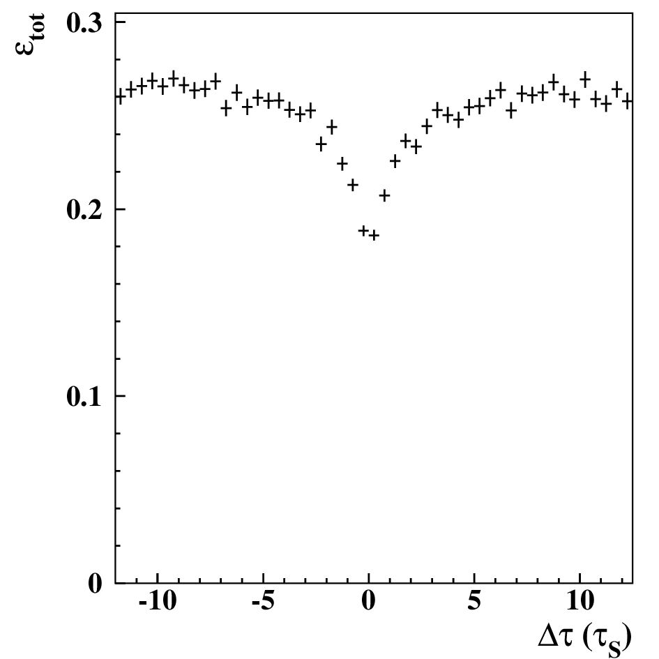
Figure 2: Left: resolution on Δ​τ\Delta\tau variable evaluated from MC simulation as the difference between true values and data-like reconstructed values. The effect of the cut on the opening angle between tracks is shown. Right: total detection efficiency as a function of true Δ​τ\Delta\tau as observed from MC simulation.The dip around Δ​τ∼0\Delta\tau\sim 0 is discussed in the text.

The main background source is the kaon regeneration on the spherical beam pipe. In order to reduce this contribution the present analysis is restricted only to events with both KS\mathrm{K}_{\mathrm{S}} and KL\mathrm{K}_{\mathrm{L}} decaying inside the beam pipe. This geometrical requirement translates in maximal absolute value for Δ​τ\Delta\tau of 12​τS12\tau_{\mathrm{S}}. In this case kaon regeneration occurs only in the thin beryllium cylinder.

The residual background contamination in the Δ​τ\Delta\tau range [−12;12]​τS[-12;12]\tau_{\mathrm{S}}, as estimated from MC simulation, is 2% from regeneration on the beryllium cylindrical foil and 0.5% e+​e−→π+​π−​π+​π−​(4​π)\mathrm{e}^{+}\mathrm{e}^{-}\rightarrow\uppi^{+}\uppi^{-}\uppi^{+}\uppi^{-}(4\uppi) direct production as estimated from a dedicated data analysis. The latter is concentrated around Δ​τ≃0\Delta\tau\simeq 0 while the former will be treated as a multiplicative correction applied to the fitting function as described in eq. (7). The 4​π4\uppi contribution is estimated to be 54±554\pm 5 events, according to Ref. [8].

For the purpose of our measurement, precise knowledge of the total detection efficiency value (εtot\varepsilon_{\mathrm{tot}}) is not required; it is however important to keep under control its dependence on Δ​τ\Delta\tau, shown in Figure 2-right. The mean value is 25% for Δ​τ\Delta\tau ranging in [−12;12]​τS[-12;12]\tau_{\mathrm{S}} with a consistent drop for Δ​τ∼0\Delta\tau\sim 0. This is due to two concurrent effects: increasing extrapolation length for tracks coming from decays very close to the beam interaction point and wrong association of tracks to the kaon decay vertices44 4 When the two vertices are so close in space (Δ​τ∼1​τS⇒Δ​λV∼6​mm\Delta\tau\sim 1\tau_{\mathrm{S}}\Rightarrow\Delta\lambda_{V}\sim 6\mathrm{mm}) it is possible to wrongly associate tracks to vertex by exchanging two of them. These vertices are then rejected because of the kinematical requirements.. The efficiency εt​o​t\varepsilon_{tot} can be divided into three main components, related to the trigger, to the reconstruction procedure and to the effect of the selection criteria:

εtot=εtrig​εreco​εcuts\varepsilon_{\mathrm{tot}}=\varepsilon_{\mathrm{trig}}\varepsilon_{\mathrm{reco}}\varepsilon_{\mathrm{cuts}}

The last contribution is derived from MC simulation while for trigger and reconstruction efficiencies, corrections obtained from real data are used. To this aim a high purity, independent control sample of KS\mathrm{K}_{\mathrm{S}}→\rightarrowπ+\uppi^{+}π−\uppi^{-} and KL\mathrm{K}_{\mathrm{L}}→\rightarrowπ\uppiμ\upmuν\upnu has been selected with particles in the same momentum range as for the signal.

The purity of the control sample is 95%, the background being dominated by Ke​3\mathrm{K}_{e3} decay. The efficiency correction has been evaluated as the ratio between data and MC distributions of IKμ​3±​(Δ​τ)I_{{K_{\mu}3}\pm}(\Delta\tau). The decay time ordering criterion is the same used in the main analysis.

Experimental data distributions have been analyzed for different intervals of sidereal time and kaon emission angle using the function in eq. (7). The Δ​τ\Delta\tau range is Δτ∈[−12:12]τS\Delta\tau\in[-12:12]\tau_{\mathrm{S}} with 1​τS1\,\tau_{\mathrm{S}} bin width, while sidereal time has 4 bins, 6 hours each, and two angular bins have been used: p→1⋅p→ϕ≷0\vec{p}_{1}\cdot{\vec{p}}_{\upphi}\gtrless 0 resulting in a total of 192 experimental points simultaneously fit. The fit χ2/NDoF\chi^{2}/N_{\mathrm{DoF}} is 211.7/187211.7/187 corresponding to a probability of 10%, numerical values of the fit are reported in Table 1 and the experimental data distributions are shown in Figure 3.

Refer to caption
Figure 3: Fit results: the top and bottom plots refer to the two angular selections. Black points are for experimental data while colored bands are the fit output. The error bars on experimental data are purely statistical, while the band represents the contribution to the uncertainty due to MC simulation statistics and efficiency correction.
Table 1: Fit results. Errors include all source of the statistical fluctuations. The fit χ2/NDoF\chi^{2}/N_{\mathrm{DoF}} is 211.7/187211.7/187 corresponding to a probability of 10%. The table contains the correlation coefficient matrix between the parameters.
Fit output (10−18​GeV10^{-18}\,\,\mathrm{GeV} units) Correlation matrix
Δ​a0\Delta a_{0}= −6.0±7.7-6.0\pm 7.7 1.000 0.304 -0.187 0.483
Δ​aX\Delta a_{\mathrm{X}}= 0.9±1.5\hphantom{-}0.9\pm 1.5 0.304 1.000 -0.045 0.069
Δ​aY\Delta a_{\mathrm{Y}}= −2.0±1.5-2.0\pm 1.5 -0.187 -0.045 1.000 -0.104
Δ​aZ\Delta a_{\mathrm{Z}}= 3.1±1.7\hphantom{-}3.1\pm 1.7 0.483 0.069 -0.104 1.000

Systematic effects are listed in Table 2. The full analysis chain has been repeated several times varying all the cuts values according to the MC resolution (σMC\sigma_{\mathrm{MC}}) of the selection variables. Positive and negative variations (±σMC\pm\sigma_{\mathrm{MC}}) have been considered. The results of the fits are stable and the RMS of the distribution of obtained results is taken as systematic uncertainty.

The accuracy on the determination of the Δ​a0\Delta a_{0} parameter strongly depends on the stability of the observed I±​(Δ​τ)I_{\pm}(\Delta\tau) distribution for |Δ​τ|>5​τS|\Delta\tau|>5\tau_{\mathrm{S}}. For this reason the fit range has been varied of ±1​τS\pm 1\tau_{\mathrm{S}} around the reference value enlarging or reducing the Δ​τ\Delta\tau range. Correspondingly the event yield varies of ∼10%\sim 10\% and the RMS of the fit results has been chosen as the related systematic error. The largest effect, as expected, has been observed on Δ​a0\Delta a_{0}.

The 4​π4\uppi background events is concentrated in the two bins around Δ​τ∼0\Delta\tau\sim 0, resulting in a bin-by-bin contribution of ∼3\sim 3 events, while the amount of observed data events in the same bins is around ∼10\sim 10 events. Being the amount of subtracted events similar to the statistical uncertainty of the observed data the systematic effect of the subtraction has been obtained as the difference between results with and without subtraction.

The effect of the orientation of the KLOE reference frame with respect to the terrestrial coordinate system has been taken into account in the fit function. The measurement of the relative alignment between our reference frame with respect to the geographical frame has been performed with a compass and the effect of displacement between magnetic and true North pole has been taken into account and corrected for. The angle between the laboratory z^\hat{z} axis and the North direction is (130±2)∘(130\pm 2)^{\circ} on the local tangent plane. The fit function has been evaluated with angle variations up to 10∘10^{\circ} showing stable results. The RMS of the results has been taken as systematic uncertainty.

The kaon regeneration correction in eq. (7) has been varied according to its relative uncertainty (∼35%\sim 35\%). The corresponding results fluctuation is negligible with respect to the other systematic uncertainty.

The effect of mismatch in Δ​τ\Delta\tau resolution between experimental data and MC simulation has been found negligible inside the maximum allowable error of 5% on Δ​τ\Delta\tau resolution width.

The final systematics uncertainty is the sum in quadrature of all the discussed effects and is reported in the last column of Table 2. In all cases the total systematic uncertainty ranges between 30% and 40% of the corresponding statistical uncertainty.

Table 2: Summary of the systematic uncertainty in 10−18​GeV10^{-18}\,\mathrm{GeV} units.
Analysis cut Δ​τ\Delta\tau Range 4​π4\pi subtr. Ref. frame Total
Δ​a0\Delta a_{0} 1.1 2.4 1.3 1.0 3.1
Δ​aX\Delta a_{\mathrm{X}} 0.3 0.3 0.4 0.2 0.6
Δ​aY\Delta a_{\mathrm{Y}} 0.2 0.3 0.2 0.2 0.5
Δ​aZ\Delta a_{\mathrm{Z}} 0.2 0.2 0.4 0.4 0.6

4 Results and conclusions

The results for the Δ​aμ\Delta a_{\mu} parameters are:

Δ​a0=(−6.0±7.7s​t​a​t±3.1s​y​s​t)×10−18​GeV\Delta a_{0}=(-6.0\pm 7.7_{stat}\pm 3.1_{syst})\times 10^{-18}\,\,\mathrm{GeV},

Δ​aX=(   0.9±1.5s​t​a​t±0.6s​y​s​t)×10−18​GeV\Delta a_{\mathrm{X}}=(\,\,\,0.9\pm 1.5_{stat}\pm 0.6_{syst})\times 10^{-18}\,\,\mathrm{GeV},

Δ​aY=(−2.0±1.5s​t​a​t±0.5s​y​s​t)×10−18​GeV\Delta a_{\mathrm{Y}}=(-2.0\pm 1.5_{stat}\pm 0.5_{syst})\times 10^{-18}\,\,\mathrm{GeV},

Δ​aZ=(   3.1±1.7s​t​a​t±0.5s​y​s​t)×10−18​GeV\Delta a_{\mathrm{Z}}=(\,\,\,3.1\pm 1.7_{stat}\pm 0.5_{syst})\times 10^{-18}\,\,\mathrm{GeV}.

The systematic uncertainty is smaller than the corresponding statistical error implying that the main limitation of the present measurement is the available statistics. To this respect the continuation of the KLOE physics program in the framework of the KLOE-2 experiment [12] at upgraded DAΦ\UpphiNE machine [14] is important to further improve the results.

The present result is the first complete measurement of all Δ​aμ\Delta a_{\mu} parameters in the kaon sector55 5 Preliminary results from KTeV collaboration in this sector can be found in the Ref. [15].. The order of magnitude of the results is approaching the interesting region defined by mK2/ℳPlank∼2×10−20​GeVm_{\mathrm{K}}^{2}/\mathcal{M}_{\mathrm{Plank}}\sim 2\times 10^{-20}\,\mathrm{GeV} in the assumption that the SME phenomenology of CPT\mathrm{CPT} and Lorentz invariance breaking is related to some underlying quantum gravity effects.

These results can be compared to similar ones for the corresponding Δ​aμ\Delta a_{\mu} parameters for the B and D neutral meson systems [16, 17] which have a precision of 𝒪⁡(10−13)\mathcal{O}(10^{-13}) GeV\mathrm{GeV}.

Acknowledgments

We warmly thank our former KLOE colleagues for the access to the data collected during the KLOE data taking campaign. We thank the DAΦ\UpphiNE team for their efforts in maintaining low background running conditions and their collaboration during all data taking. We want to thank our technical staff: G.F. Fortugno and F. Sborzacchi for their dedication in ensuring efficient operation of the KLOE computing facilities; M. Anelli for his continuous attention to the gas system and detector safety; A. Balla, M. Gatta, G. Corradi and G. Papalino for electronics maintenance; M. Santoni, G. Paoluzzi and R. Rosellini for general detector support; C. Piscitelli for his help during major maintenance periods. We acknowledge the support of the European Community – Research Infrastructure Integrating Activity ‘Study of Strongly Interacting Matter’ (acronym HadronPhysics2, Grant Agreement No. 227431) under the Seventh Framework Programme of EU. This work was supported also in part by the EU Integrated Infrastructure Initiative Hadron Physics Project under contract number RII3-CT-2004-506078; by the European Commission under the 7th Framework Programme through the ‘Research Infrastructures’ action of the ‘Capacities’ Programme, Call: FP7-INFRASTRUCTURES- 2008-1, Grant Agreement No. 283286; by the Polish National Science Centre through the Grants No. 0469/B/H03/2009/37, 0309/B/H03/2011/40, DEC-2011/03/N/ST2/02641, 2011/01/D/ST2/00748, 2011/03/N/ST2/02652,2011/03/N/ST2/02641, 2013/08/M/ST2/00323 and by the Foundation for Polish Science through the MPD programme and the project HOMING PLUS BIS/2011-4/3.

References

  • [1] G. Lueders, Ann. Phys. (NY) 2 (1957) 1, reprinted in Ann. Phys. (NY) 281 (2000) 1004; W. Pauli, Exclusion principle, Lorentz group and reflexion of space-time and charge in Niels Bohr and the development of physics, edited by W. Pauli, Pergamon, London, 1955, p.30; J. S. Bell, Proc. R. Soc. London A 231 (1955) 479; R. Jost, Helv. Phys. Acta 30 (1957) 409.
  • [2] O. W. Greenberg, Phys. Rev. Lett. 89 (2002) 231602.
  • [3] V. A. Kostelecký and S. Samuel, Phys. Rev. D 39, 683 (1989);
    V. A. Kostelecký and R. Potting, Nucl. Phys. B 359, 545 (1991).
  • [4] D. Colladay and V. A. Kostelecký,Phys. Rev. D 55 (1997) 6760;
    D. Colladay and V. A. Kostelecký,Phys. Rev. D 58 (1998) 116002;
    V. A. Kostelecký and R. Potting, Phys. Rev. D 51 (1995) 3923.
  • [5] V. A. Kostelecký and N. Russell, Rev. Mod. Phys. 83 (2011) 11, (Updates on [arXiv:0801.0287 [hep-ph]]).
  • [6] V. A. Kostelecký, Phys. Rev. Lett. 80, 1818 (1998);
    V. A. Kostelecký, Phys. Rev. D 61, 016002 (1999);
    V. A. Kostelecký, Phys. Rev. D 64, 076001 (2001).
  • [7] A. Di Domenico (Editor), Handbook on Neutral Kaon Interferometry at a ϕ\phi-factory, Frascati Phys. Ser. 43 (2007).
  • [8] F. Ambrosino et al. [KLOE Coll.], Phys. Lett. B 642 (2006) 315.
  • [9] M. Adinolfi et al., Nucl. Inst. Meth. A 488 (2002) 51.
  • [10] A. Balla, M. Beretta, P. Branchini, P. Ciambrone, G. Corradi, E. De Lucia, P. De Simone and G. Felici et al., Nucl. Instrum. Meth. A 562 (2006) 141.
  • [11] M. Adinolfi et al., Nucl. Instrum. Meth. A 482 (2002) 363.
  • [12] G. Amelino-Camelia et al., Eur. Phys. J. C 68 (2010) 619.
  • [13] F. Ambrosino, et al., [KLOE Coll.] Nucl. Instrum. Meth. A 534 (2004) 403.
  • [14] M. Zobov, D. Alesini, M. E. Biagini, C. Biscari, A. Bocci, M. Boscolo, F. Bossi and B. Buonomo et al., Phys. Rev. Lett. 104 (2010) 174801.
  • [15] H. Nguyen, “CPT results from KTeV,” unpublished, [hep-ex/0112046].
  • [16] B. Aubert et al. [BaBar Coll.], Phys. Rev. Lett. 100 (2008) 131802.
  • [17] J. M. Link, et al.[FOCUS Coll.], Phys. Lett. B 556 (2003) 7.