New explicit thresholding/shrinkage formulas for one class of regularization problems with overlapping group sparsity and their applicationsThanks: The work of Gang Liu, Ting-Zhu Huang and Jun Liu is supported by 973 Program (2013CB329404), NSFC (61370147), Sichuan Province Sci. & Tech. Research Project (2012GZX0080). The work of Xiao-Guang Lv is supported by Postdoctoral Research Funds (2013M540454, 1301064B).

For the original sparse represent solutions we often want to solve the following problems

Definition 1. Define shrinkage mappings $Sh_{1}$ and $Sh_{2}$ from $\mathbb{R}^{N}\times R^{+}$ to $\mathbb{R}^{N}$ by

where both expressions are taken to be zero when the second factor is zero, and “sgn” represents the signum function indicating the sign of a number, that is, sgn($x$)=0 if $x=0$, sgn($x$)=-1 if $x<0$ and sgn($x$)=1 if $x>0$.

The shrinkage (7) is known as soft thresholding and occurs in many algorithms related to sparsity since it is the proximal mapping for the $\ell_{1}$ norm. Then the minimizer of (6) with $p=1$ is the following equation (9).

Thanks to the additivity and separability of both the $\ell_{1}$ norm and the square of the $\ell_{2}$ norm, the shrinkage (7) can be deduced easily by the following formula:

The minimizer of (6) with $p=2$ is the following equation (11).

This formula is deduced by the Euler equation of (6) with $p=2$. Clearly,

We can easily get that the necessary condition is that the vector $\mathbf{z}$ is parallel to the vector $\mathbf{x}$. That is $\frac{\mathbf{z}}{\|\mathbf{z}\|_{2}}=\frac{\mathbf{x}}{\|\mathbf{x}\|_{2}}$. Substitute into (13), and the formula (8) is obtained. More details please refer to [37, 38].

Our new explicit OGS shrinkage formulas are based on these observations, especially the properties of additivity, separability and parallelity.
Remark 1. The problem (2) is also easy to be solved by a simple shrinkage formula, which is not used in this work. More details refer to [8, 35, 34].

Now we focus on the problem (3) firstly. The difficulty of this problem is overlapping. Therefore, we must take some special techniques to avoid overlapping. That is the point of our new explicit OGS shrinkage formulas.

It is obvious that the first term of the problem (3) is additive and separable. So if we find some relative rules such that the second term of the problem (3) has the same properties with the same variable as the first term, the solution of (3) can be easily found similar as (10).

Assuming period boundary conditions is used here, we observe that each entry $z_{i}$ of vector $\mathbf{z}$ would appear exactly $s$ times in the first term. Therefore, to hold on the uniformity of vectors $\mathbf{z}$ and $\mathbf{x}$, we need multiply the second term by $s$. To maintain the invariability of the problem (3), and after some manipulations, we have

where $(x_{i})_{g}$ is same as $(z_{i})_{g}$ defined before.

For example, we set $s=3$ and define $(z_{i})_{g}=(z_{i},z_{i+1},z_{i+2})$. The generalized $\ell_{2,1}$-norm $\|\mathbf{z}\|_{2,1}$ can be treated as the generalized $\ell_{1}$ norm of generalized points, whose entry $(z_{i})_{g}$ is also a vector, and the absolute value of each entry is treated as the $\ell_{2}$ norm of $(z_{i})_{g}$. See Figure 1(a) intuitively, where the top line is the vector $\mathbf{z}$, the rectangles with dashed line are original $(z_{i})_{g}$, and the rectangles with solid line are the generalized points. Because of the period boundary conditions, we know that each line of Figure 1(a) is translated equal. We treat the vector $\mathbf{x}$ same as the vector $\mathbf{z}$. Putting these generalized points (rectangles with solid line in the figure) as the columns of a matrix, then $s\|\mathbf{z}-\mathbf{x}\|_{2}^{2}$ can be regarded as matrix Frobenius norm $\|\left((z_{i})_{g}\right)-\left((x_{i})_{g}\right)\|_{F}$ in Figure 1(a) with every line being the row of the matrix. This is why the second equality in (14) holds. Therefore, generally, for each $i$ of the last line of (14), from the equation (8) and (11), we can obtain

then

Similarly as Figure 1(a), for each $i$, the $i$th entry $x_{i}$ (or $z_{i}$) of the vector $\mathbf{x}$ (or $\mathbf{z}$) may appear $s$ times, so we need compute each $z_{i}$ for $s$ times in $s$ different groups.

However, the results from (15) are wrong, because the results $z_{i}$ in $s$ different groups are different from (15). That means the results are not able to be satisfied simultaneously in this way. Moreover, for each $i$ of the last line in (14), the result (15) is given by that the vector $(z_{i})_{g}$ is parallel to the vector $(x_{i})_{g}$. Notice this point and ignore that $(z_{i})_{g}=\mathbf{0}$ or $(x_{i})_{g}=\mathbf{0}$, particularly for $s=4$ and $(z_{i})_{g}=(z_{i-1},z_{i},z_{i+1},z_{i+2})$, the vector $\mathbf{z}$ can be split as follows,

Let $(z_{i})^{\prime}_{g}=(0,\cdots,0,z_{i-1},z_{i},z_{i+1},z_{i+2},0,\cdots,0)$ be the expansion of $(z_{i})_{g}$, with $(z_{1})^{\prime}_{g}=(z_{1},z_{2},z_{3},0,$ $\cdots,0,z_{n})$, $(z_{n-1})^{\prime}_{g}=(z_{1},0,0,\cdots,0,z_{n-2},z_{n-1},z_{n})$, $(z_{n})^{\prime}_{g}=(z_{1},z_{2},0,\cdots,0,z_{n-1},z_{n})$. Let $(x_{i})^{\prime}_{g}=(0,\cdots,0,x_{i-1},x_{i},x_{i+1},x_{i+2},0,\cdots,0)$ be the expansion of $(x_{i})_{g}$ similarly as $(z_{i})^{\prime}_{g}$. Then, we have $\mathbf{z}=\frac{1}{4}\sum_{i=1}^{n}(z_{i})^{\prime}_{g}$, and $\mathbf{x}=\frac{1}{4}\sum_{i=1}^{n}(x_{i})^{\prime}_{g}$. Moreover, we can easily obtain that $\|(z_{i})^{\prime}_{g}\|_{2}=\|(z_{i})_{g}\|_{2}$ and $\|(x_{i})^{\prime}_{g}\|_{2}=\|(x_{i})_{g}\|_{2}$ for every $i$.

On one hand, the Euler equation of $f_{m}(\mathbf{z})$ (with $s=4$) is given by

From the deduction of the 2-dimensional shrinkage formula (8) in Section 2.1, we know that the necessary condition of minimizing the $i$th term of the last line in (14) is that $(z_{i})_{g}$ is parallel to $(x_{i})_{g}$. That is, $(z_{i})^{\prime}_{g}$ is parallel to $(x_{i})^{\prime}_{g}$ for every $i$. For example,

Then we obtain $\frac{(z_{i})^{\prime}_{g}}{\|(z_{i})^{\prime}_{g}\|_{2}}=\frac{(x_{i})^{\prime}_{g}}{\|(x_{i})^{\prime}_{g}\|_{2}}$. Therefore, (18) changes to

for each component, we obtained

Therefore, when $(z_{i})_{g}\neq\mathbf{0}$ and $(x_{i})_{g}\neq\mathbf{0}$, we find a minimizer of (3) on the direction that all the vectors $(z_{i})_{g}$ are parallel to the vectors $(x_{i})_{g}$. In addition, when $\frac{\beta}{4}\left((z_{i})^{\prime}_{g}-(x_{i})^{\prime}_{g}\right)+\frac{(z_{i})^{\prime}_{g}}{\|(z_{i})^{\prime}_{g}\|_{2}}=0$, (18) holds, then $\left(\frac{\beta}{4}+\frac{1}{\|(z_{i})^{\prime}_{g}\|_{2}}\right)(z_{i})^{\prime}_{g}=(x_{i})^{\prime}_{g}$, therefore, $\frac{(z_{i})^{\prime}_{g}}{\|(z_{i})^{\prime}_{g}\|_{2}}=\frac{(x_{i})^{\prime}_{g}}{\|(x_{i})^{\prime}_{g}\|_{2}}$ holds. Moreover, because of the strict convexity of $f_{m}(\mathbf{z})$, we know that the minimizer is unique. This minimizer $\mathbf{z}$ is accurate.

On the other hand, when $(z_{i})_{g}=\mathbf{0}$ or $(x_{i})_{g}=\mathbf{0}$, our method may not obtain the accurate minimizer. When $(x_{i})_{g}=\mathbf{0}$, we know that the minimizer of the subproblem $\min\limits_{(z_{i})_{g}}\|(z_{i})_{g}\|_{2}+\frac{\beta}{2s}\|(z_{i})_{g}-(x_{i})_{g}\|_{2}^{2}$ is exactly that $(z_{i})_{g}=\mathbf{0}$. When $(x_{i})_{g}\neq\mathbf{0}$ and the minimizer of the subproblem $\min\limits_{(z_{i})_{g}}\|(z_{i})_{g}\|_{2}+\frac{\beta}{2s}\|(z_{i})_{g}-(x_{i})_{g}\|_{2}^{2}$ is that $(z_{i})_{g}=\mathbf{0}$ (this is because that the parameter $\beta/s$ is two small), our method is not able to obtain the accurate minimizer. For example, that $(z_{i})_{g}=\mathbf{0}$ while $(z_{i+1})_{g}\neq\mathbf{0}$ makes the element $z_{i}$ in $\mathbf{z}$ take different values in different subproblems. However, we can obtain an approximate minimizer in this case, which is that the element $z_{i}$ is a simple summation of corresponding subproblems containing $z_{i}$. We will show that in experiments of Section 5 the approximate minimizer is also good. Moreover, when we take this problem as a subproblem of the image processing problem, we can set the parameter $\beta$ to be large enough to make sure that the minimizer of the subproblem is accurate. Therefore, the convergence theorem results can be obtained by this accuracy, which will be applied in Section 4.

In addition, form (23), we can know that the element $z_{i}$ of the minimizer can be treated as in $s$ subproblems independently and then combine them. After some manipulations, in conclusion, we can get the following two general formulas.

1).

with

Here, for instance, when group size $s=4$, $(z_{i})_{g}=(z_{i-1},z_{i},z_{i+1},z_{i+2})$ in $\|\mathbf{z}\|_{2,1}$ and $(x_{i})_{g}$ is defined similarly as $(z_{i})_{g}$, we have $F(x_{i})=\left(\frac{1}{\|(x_{i-2})_{g}\|_{2}}+\frac{1}{\|(x_{i-1})_{g}\|_{2}}+\frac{1}{\|(x_{i})_{g}\|_{2}}+\frac{1}{\|(x_{i+1})_{g}\|_{2}}\right)$. The $\|(x_{j})_{g}\|_{2}$ is contained in $F(x_{i})$ if and only if $\|(x_{j})_{g}\|_{2}$ has the component $x_{i}$, and we follow the convention $(1/0)=1$ in $F(x_{i})$ because $\|(x_{i})_{g}\|_{2}=0$ implies $x_{i}=0$ and the value of $F(x_{i})$ is insignificant in (25).

2).

with

Here, symbols are the same as 1), and $G(x_{i})=\max\left(\frac{1}{s}-\frac{1}{\beta\|(x_{i-2})_{g}\|_{2}},0\right)$ $+\max\left(\frac{1}{s}-\frac{1}{\beta\|(x_{i-1})_{g}\|_{2}},0\right)$
$+\max\left(\frac{1}{s}-\frac{1}{\beta\|(x_{i})_{g}\|_{2}},0\right)+\max\left(\frac{1}{s}-\frac{1}{\beta\|(x_{i+1})_{g}\|_{2}},0\right)$.

When $\beta$ is sufficiently large or sufficiently small, the former two formulas are the same and both are accurate. For the other values of $\beta$ , from the experiments, we find that 2) is better approximate than 1), so we choose the formula 2). Then, we obtain the following algorithm for finding the minimizer of (3).
Algorithm 1 Direct shrinkage algorithm for the minimization problem (3) Input:    Given vector $\mathbf{x}=(x_{1},x_{2},\cdots,x_{n})$, group size $s$, parameter $\beta$. Compute: Definition of $(x_{i})_{g}$, for example $(x_{i})_{g}=\left(x_{i-s_{l}},\cdots,x_{i},\cdots,x_{i+s_{r}}\right)$, with $s_{l}=[\frac{s-1}{2}]$ and $s_{r}=[\frac{s}{2}]$ ($s_{l}+s_{r}+1=s$). $\mathbf{w}$ = ones(1,s) = [1,1,$\cdots$,1]. If $s$ is even, then $\mathbf{w}=[\mathbf{w},0]$ and $s=s+1$. Let $\mathbf{w}_{r}$ = fliplr($\mathbf{w}$) be fliping $\mathbf{w}$ over 180 degrees. Compute $X_{n}=\left(\|(x_{1})_{g}\|_{2},\cdots,\|(x_{i})_{g}\|_{2},\cdots,\|(x_{n})_{g}\|_{2}\right)$, by convolution of $\mathbf{w}$ and $\mathbf{x}$. Compute $X^{\prime}_{n}=\max\left(\frac{1}{s}-1./(X_{n}\cdot\beta),0\right)$ pointwise. Compute $G(x_{i})$ by correlation of $\mathbf{w}$ and $X^{\prime}_{n}$, or by convolution of $\mathbf{w}_{r}$ and $X^{\prime}_{n}$.

We can see that Algorithm 1 only need 2 times convolution computations with time complexity $n*s$, which is just the same time complexity as one step iteration in the MM method in [4]. Therefore, our method is much more efficient than MM method or other variable duplication methods. In Section 5, we will give the numerical experiments for comparison between our method and the MM method. Moreover, if $s=1$, our Algorithm 1 degenerates to the classic soft thresholding as our formula (27) degenerates to (7). Moreover, when $\beta$ is sufficiently large or sufficiently small, our algorithm is accurate while MM method is also approximate.
Remark 2 Our new explicit algorithm can be treated as an average estimation algorithm for solve all the overlapping group subproblem independently. In Section 5, our numerical experiments show that Our new explicit algorithm is accurate when $\beta$ is sufficiently large or sufficiently small, and is approximate to the other methods for instance the MM method for other $\beta$.

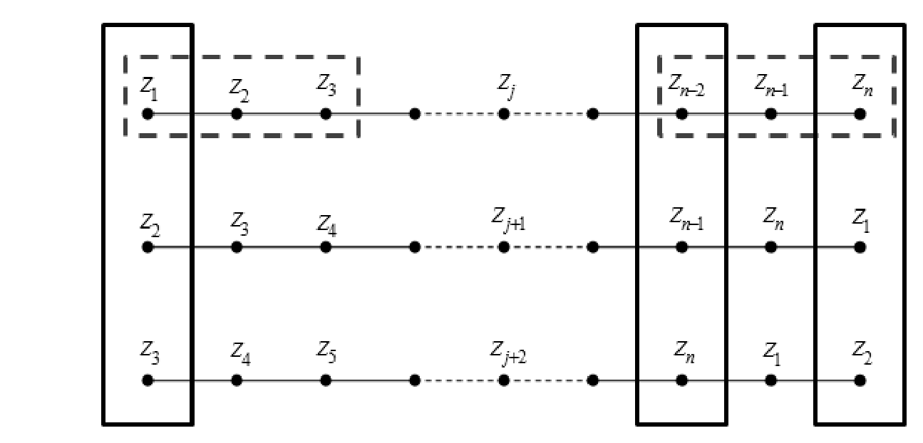
For the problem (4), similar to (14), we can get

See Figure 1(b) intuitively. All the symbols are the same as before. Similarly as before, we know that the necessary condition of minimizing the $i$th term of the last line in (28) is that ($w_{g}\circ(z_{i})_{g}$) is parallel to ($w_{g}\circ(x_{i})_{g}$). That is, $\frac{w_{g}\circ(z_{i})_{g}}{\|w_{g}\circ(z_{i})_{g}\|_{2}}=\frac{w_{g}\circ(x_{i})_{g}}{\|w_{g}\circ(x_{i})_{g}\|_{2}}$ for every $i$. On the other hand, Let $W$=diag($w_{g}$) be a diagonal matrix with diagonal being the vector $w_{g}$, then $w_{g}\circ(x_{i})_{g}=W(x_{i})_{g}=W^{T}(x_{i})_{g}$. If the vector $\mathbf{x^{\prime}}$ (the same size as $(x_{i})_{g}$) is parallel to the vector $\mathbf{z^{\prime}}$, we have $\mathbf{x^{\prime}}=\alpha\mathbf{z^{\prime}}$. Then, $W\mathbf{x^{\prime}}=W\alpha\mathbf{z^{\prime}}=\alpha W\mathbf{z^{\prime}}$. We obtain that the vector $W\mathbf{x^{\prime}}$ is also parallel to the vector $W\mathbf{z^{\prime}}$. Therefore, $\frac{W(z_{i})_{g}}{\|W(z_{i})_{g}\|_{2}}=\frac{W(x_{i})_{g}}{\|W(x_{i})_{g}\|_{2}}$, and each of them is a unit vector. Then, $\frac{W^{T}W(z_{i})_{g}}{\|W(z_{i})_{g}\|_{2}}=\frac{W^{T}W(x_{i})_{g}}{\|W(x_{i})_{g}\|_{2}}$. That is,

Particularly, we first consider that $s=4$, $(z_{i})_{g}=(z_{i-1},z_{i},z_{i+1},z_{i+2})$ and $w_{g}=(w_{1},w_{2},w_{3},w_{4})$. We mark $(w_{g}\circ(z_{i})_{g})^{\prime}$ be the expansion of ($w_{g}\circ(z_{i})_{g}$) similarly as $(z_{i})_{g}^{\prime}$, and we can get $\mathbf{x}=\frac{1}{\sum_{i=1}^{4}w_{i}}\sum_{i=1}^{n}(w_{g}\circ(z_{i})_{g})^{\prime}$. Then, the Euler equation of $f_{w}(\mathbf{z})$ is given by

References

- [1] I. Bayram, Mixed norms with overlapping groups as signal priors, IEEE Int. Conf. Acoust., Speech, Signal Processing (ICASSP), pp. 4036¨C4039, (May, 2011).
- [2] F. Bach, R. Jenatton, J. Mairal and G. Obozinski, Structured sparsity through convex optimization, Technical Report, Hal-00621245, (2011).
- [3] A. Chambolle, An algorithm for total variation minimization and applications, J. Math. Imaging Vis., 20, pp. 89–97, (2004).
- [4] P. -Y. Chen and I. W. Selesnick, Translation-invariant shrinkage/thresholding of group sparse signals, Signal Processing, 94, pp. 476–489, (2014).
- [5] W. Cao, J. Sun and Z. Xu, Fast image deconvolution using closed-Form thresholding formulas of regularization, J. Vis. Commun. Image. R., 24, pp. 31–41, (2012).
- [6] R. Chan, M. Tao and X. M. Yuan, Constrained total variational deblurring models and fast algorithms based on alternating direction method of multipliers, SIAM J. Imaging Sci., 6, pp. 680–697, (2013).
- [7] R. Chartrand, B. Wohlberg, A nonconvex ADMM algorithm for group sparsity with sparse groups, IEEE Int. Conf. Acoust., Speech, Signal Processing (ICASSP), (May, 2013).
- [8] W. Deng, W. Yin and Y. Zhang, Group sparse optimization by alternating direction method, Proc. SPIE 8858, Wavelets and Sparsity XV, 88580R, (September, 2013), http://dx.doi.org/10.1117/12.2024410.
- [9] E. Esser, Applications of Lagrangian-based alternating direction methods and connections to split Bregman, UCLA CAM report, pp. 9–31, (2009).
- [10] J. Eckstein and D. Bertsekas, On the Douglas-Rachford splitting method and the proximal point algorithm for maximal monotone operators, Math. Program., 55, pp. 293–318, (1992).
- [11] E. Elhamifar and R. Vidal, Robust classification using structured sparse representation, IEEE Conf. Computer Vision and Pattern Recognition (CVPR), pp. 1873–1879, (2011).
- [12] M. Figueiredo and J. Bioucas-Dias, An alternating direction algorithm for (overlapping) group regularization, Signal Processing with Adaptive Sparse Structured Representations (SPARS), (2011).
- [13] R. Glowinski, Lectures on numerical methods for nonlinear variational problems, Springer, New York, (2008).
- [14] J. C. Gilbert and C. Lemaréchal, Numerical optimization: theoretical and practical aspects, Springer, (2006).
- [15] D. Gabay and B. Mercier, A dual algorithm for the solution of nonlinear variational problems via finite-element approximations, Comput. Math. Appl., 2, pp. 17–40, (1976).
- [16] J. Gao, Q. Shi and T. S. Caetano, Dimensionality reduction via compressive sensing, Pattern Recognit. Lett., 33, pp. 1163–1170, (2012).
- [17] P. C. Hansen, J. G. Nagy and D. P. O’Leary, Deblurring images: matrices, spectra, and filtering, SIAM, Philadelphia, (2007).
- [18] B. He and H. Yang, Some convergence properties of a method of multipliers for linearly constrained monotone variational inequalities, Operations research letters, 23, pp. 151–161, (1998).
- [19] J. Huang and T. Zhang, The benefit of group sparsity, Ann. Statist., 38, pp. 1978–2004, (2010).
- [20] R. Jenatton, J.-Y. Audibert and F. Bach, Structured variable selection with sparsity-inducing norms, Journal of Machine Learning Research, 11, pp. 2777¨C2824, (October, 2011).
- [21] L. Jacob, G. Obozinski and J. Vert, Group Lasso with overlap and graph Lasso, International Conference on Machine Learning, pp. 433–440, (2009).
- [22] M. Kowalski, Sparse regression using mixed norms, Journal of Applied and Computational Harmonic Analysis, 27, pp. 303¨C324, (2009).
- [23] D. Krishnan and R. Fergus, Fast image deconvolution using hyper-laplacian priors, Advances in Neural Information Processing Systems (NIPS), pp. 1033–1041, (2009).
- [24] G. Liu, T.-Z Huang, J. Liu and X. G. Lv, Total variation with overlapping group sparsity gor image deblurring under impulse noise, arXiv preprint arXiv:1312.6208, (2013).
- [25] J. Liu , T.-Z Huang, I. W. Selesnick, X. G. Lv and P. Chen, Image restoration using total variation with overlapping group sparsity, arXiv preprint arXiv:1310.3447, (2013).
- [26] Y. Liu, F. Wu and Y. Zhuang, Group sparse representation for image categorization and semantic video retrieval, Sci. China Inform. Sci., 54, pp. 2051–2063, (2011).
- [27] R. Mazumder, J. H. Friedman and T. Hastie, SparseNet: coordinate descent with non-convex penalties. Journal of the American Statistical Association, 106(495), pp. 1125¨C1138, (2011).
- [28] A. Majumdar and R. K. Ward, Classification via group sparsity promoting regularization, IEEE Int. Conf. Acoust., Speech, Signal Processing (ICASSP), pp. 861–864, (2009).
- [29] M. K. Ng, P. Weiss and X. Yuan, Solving constrained total-variation image restoration and reconstruction problems via alternating direction methods, SIAM J. Sci. Comput., 32, pp. 2710–2736, (2010).
- [30] G. Peyre and J. Fadili, Group sparsity with overlapping partition functions, Proceedings of the European Signal Processing Conference (EUSIPCO), (August. 29-September. 2, 2011).
- [31] L. Rudin, S. Osher and E. Fatemi, Nonlinear total variation based noise removal algorithms, Physica D., 60, pp. 259–268, (1992).
- [32] I. W. Selesnick and P. -Y Chen, Total variation denoising with overlapping group sparsity, IEEE Int. Conf. Acoust., Speech, Signal Processing (ICASSP), (May, 2013).
- [33] M. Stojnic, F. Parvaresh and B. Hassibi, On the reconstruction of block-sparse signals with an optimal number of measurements, IEEE Trans. Signal Process., 57, pp. 3075–3085, (2009).
- [34] P. Sprechmann, I. Ramirez, G. Sapiro and Y. C. Eldar, C-HiLasso: A collaborative hierarchical sparse modeling framework, IEEE Trans. Signal Process., 59, pp. 4183–4198, (2011).
- [35] B. Wohlberg, R. Chartrand and J. Theiler, Local principal component pursuit for nonlinear datasets, IEEE Int. Conf. Acoust., Speech, Signal Processing (ICASSP), pp. 3925–3928, 2012.
- [36] C. L. Wu and X. -C. Tai, Augmented Lagrangian method, dual methods, and split Bregman iteration for ROF, vectorial TV, and high Order Models, SIAM J. Imaging Sci., 3, pp. 300–339, (2010).
- [37] Y. Wang, J. Yang, W. Yin and Y. Zhang, A new alternating minimization algorithm for total varization image reconstruction, SIAM J. Imaging Sci., 1, pp. 248–272, (2008).
- [38] J. Yang, W. Yin, Y. Zhang and Y. Wang, A fast algorithm for edge-preserving variational multichannel image restoration, SIAM J. Imaging Sci., 2, pp. 569–592, (2009).
- [39] J. Yang, Y. Zhang and W. Yin, A fast alternating direction method for TVL1-L2 signal reconstruction from partial Fourier data, IEEE J. Sel. Topics Signal Process., 4, pp. 288–297, (2010).
- [40] X. Zhang, M. Burger, X. Bresson and S. Osher, Bregmanized nonlocal regularization for deconvolution and sparse reconstruction, SIAM J. Imaging Sci., 3, pp. 253–276, (2010).
- [41] X. Zhang, M. Burger and S. Osher, A unified primal-dual algorithm framework based on Bregman iteration, J. Sci. Comput., 46, pp. 20–46, (2010).