![[Uncaptioned image]](1312.6540v1/orbit10.png)
Supersymmetric rotating black hole spacetime tested by geodesics
Abstract
We present the complete analytical solution of the geodesics equations in the supersymmetric BMPV spacetime [1]. We study systematically the properties of massive and massless test particle motion. We analyze the trajectories with analytical methods based on the theory of elliptic functions. Since the nature of the effective potential depends strongly on the rotation parameter , one has to distinguish between the underrotating case, the critical case and the overrotating case, as discussed by Gibbons and Herdeiro in their pioneering study [2]. We discuss various properties which distinguish this spacetime from the classical relativistic spacetimes like Schwarzschild, Reissner-Nordström, Kerr or Myers-Perry. The overrotating BMPV spacetime allows, for instance, for planetary bound orbits for massive and massless particles. We also address causality violation as analyzed in [2].
pacs
04.20.Jb, 02.30.HqI Introduction
The Breckenridge-Myers-Peet-Vafa (BMPV) spacetime [1] represents a fascinating solution of the bosonic sector of minimal supergravity in five dimensions. It describes a family of charged rotating extremal black holes with equal-magnitude angular momenta, that are associated with independent rotations in two orthogonal planes.
The BMPV solution has been analyzed in various respects. At first interest focussed on the entropy of the extremal black hole solutions. Here a microscopic derivation of the entropy led to perfect agreement with the classical value obtained from the horizon area of the black holes , where is a charge parameter and is the rotation parameter [1]. Clearly, the entropy is largest in the static case, and vanishes in the critical case . For still faster rotation the radicant would become negative.
Gauntlett, Myers and Townsend [3] analyzed the BMPV spacetime further, pointing out that it describes supersymmetric black hole solutions with a non-rotating horizon, but finite angular momentum. They argued that angular momentum can be stored in the gauge field, and a negative fraction of the total angular momentum resides behind the horizon, while the effect of the rotation on the horizon is to make it squashed [3].
While Gauntlett, Myers and Townsend [3] addressed already the presence of closed timelike curves (CTSs) in the BMPV spacetime, a thorough qualitative study of the geodesics and the possibility of time travel was given by Gibbons and Herdeiro [2]. Considering three cases for the BMPV spacetime, Gibbons and Herdeiro pointed out, that while in the underrotating case the CTCs are hidden behind the degenerate horizon, the CTCs occur in the exterior region in the overrotating case. Thus the BMPV spacetime contains naked time machines in this case.
Moreover, in the overrotating case the horizon becomes ill-defined, since it becomes a timelike hypersurface, with the entropy becoming naively imaginary [2, 4, 5, 6]. This hypersurface is then referred to as pseudo-horizon. In fact, as shown by Gibbons and Herdeiro, this pseudo-horizon cannot be traversed by particles or light following geodesics. Thus the interior region of an overrotating BMPV spacetime cannot be entered. Therefore the outer spacetime represents a repulson. The geodesics in the exterior region between the pseudo-horizon and infinity are complete.
The repulson behavior of the overrotating BMPV spacetime has been analyzed further by Herdeiro [4]. By studying the motion of charged testparticles in the spacetime he realized that the repulson effect is still present. Considering accelerated observers, however, he noted that it could be possible to travel into the interior region [4].
Herdeiro further showed, that when oxidising the overrotating BMPV solution to the causal anomalies are resolved. Interestingly, here a relation between microscopic unitarity and macroscopic causality emerged. The breakdown of causality in the BMPV spacetime is associated with a breakdown of unitarity in the super conformal field theory [4, 5] (see also [7]).
The BMPV solution may be considered as a subset of a more general family of solutions found by Chong, Cvetic, Lü and Pope [8]. This more general family of solutions exhibits close similarities and, in particular, a generic presence of CTCs. However, it also contains further supersymmetric black holes, where naked CTCs can be avoided, and in addition new topological solitons.
Along these lines Cvetic, Gibbons, Lü and Pope [6] gave a thorough analysis of further exact solutions of gauged supergravities in four, five and seven dimensions. Again, these solutions in general may possess CTCs, but interesting regular black hole and soliton solutions are present as well.
Here we revisit the properties of the BMPV spacetime by constructing the complete analytical solution of the geodesic equations in this spacetime. We systematically study the motion of massive and massless test particles and analyze the trajectories with analytical methods based on the theory of elliptic functions. We classify the possible orbits and present examples of these orbits to illustrate the various types of motion.
Our paper is structured as follows. In section II we introduce and discuss the metric of the BMPV spacetime. We present the Kretschmann scalar, which reveals the physical singularity at (in our coordinates). Subsequently, we here derive the equations of motion.
In section III.1 we discuss the properties of the -motion and derive the solution of the -equation. In section III.2 we solve the radial equation in terms of the Weierstrass’ -function. We then discuss in detail the properties of the motion in terms of the effective potential in subsection III.2.1. We distinguish between the underrotating case, the overrotating case and the critical case, which are definded in terms of the values of the rotation parameter . We then discuss the corresponding dynamics of massive and massless test particles for these cases. In subsection III.2.6 we exemplify the properties of motion with parameteric diagrams from the radial polynomial.
In section III.3 and section III.4 we solve the differential equations for the and equations in terms of Weierstrass’ functions. We solve the equation in section III.5. In section III.6 we address causality. To illustrate our analytical solutions we present in section IV various types of trajectories. We show two-dimensional orbits in the plane in section IV.1, and three-dimensional projections of four-dimensional orbits in section IV.2. In the last section we conclude.
II The metric and the equations of motion
II.1 The metric
The five dimensional metric describing the BMPV spacetime can be expressed as follows [1]
| (1) |
The parameter is related to the charge and to the mass of these solutions, while the parameter is related to their two equal magnitude angular momenta. The coordinates , , , represent a spherical coordinate system, where the angular coordinates have the ranges , and .
It is convenient to work with a normalized metric of the form
| (2) |
with dimensionsless coordinates and parameter
| (3) |
Note, that in order to avoid a complicated notation we retain the same notation for the normalized coordinates and quantities.
The BMPV spacetime is a stationary asymptotically flat spacetime. It has two hypersurfaces relevant for its physical interpretation in the following discussion. The hypersurface where vanishes looks like a non-rotating degenerate horizon located at . The second hypersurface is associated with the causal properties of the spacetime. Representing the outer boundary of the region where CTCs arise, it is located at and referred to as the velocity of light surface (VLS) [2, 4, 5, 6].
For the proper description of the BMPV spacetime we need to distinguish the following three cases:
- 1.
: underrotating case
- 2.
: critical case
- 3.
: overrotating case
In the underrotating case the BMPV spacetime describes extremal supersymmetric black holes. Here indeed a degenerate horizon is located at , and the VLS is hidden behind the horizon. Since CTCs arise only inside the VLS, the black hole spacetime outside the horizon is free of CTCs.
In the overrotating case the surface becomes a timelike hypersurface. Therefore this surface does not describe a horizon. It is referred to as a pseudo-horizon, whose area would be imaginary. In the overrotating case the VLS resides outside the surface . Thus the outer spacetime contains a naked time machine. Since no geodesics can cross the pseudo-horizon, the spacetime represents a repulson [2, 4, 5, 6].
In the critical case the surface has vanishing area. Here the VLS coincides with this surface . Thus there is no causality violation in the outer region .
The Kretschmann scalar , where are the contravariant components of the Riemann tensor, in the BMPV spacetime has the form
| (4) |
which indicates that the spacetime has a physical point-like singularity at . At the Kretschmann scalar is finite.
Our detailed analytical study of the geodesics of neutral particles and light in the BMPV spacetime fully supports the previous analysis of the properties of this spacetime.
II.2 The Hamilton-Jacobi equation
The Hamilton-Jacobi equation for neutral test particles is of the form (see e.g. [9])
| (5) |
We therefore need the non-vanishing inverse metric components given by
| (6) |
We search for the solution of the equations (5) in the form:
| (7) |
where is the conserved energy of a test particle with a mass parameter , and and are its conserved angular momenta. for massless test particles and for massive test particles. Since the metric components are functions of the coordinates and , we have to separate the equations of motion with respect to these coordinates. is an affine parameter.
Since the left and right hand sides of the equation (8) depend only on and , respectively, we can equate both sides to a constant , the separation constant. We obtain
| (9) | |||||
| (10) |
where we have introduced new functions and .
We can write the action (equation (7)) in the form
| (11) |
Following the standard procedure we differentiate equation (11) with respect to the constants , , , and . The result is a constant which can be set zero. Combining the derived differential equations we get the Hamilton-Jacobi equations in the form
| (12) | |||
| (13) | |||
| (14) | |||
| (15) | |||
| (16) |
where and are given by (9) and (10), and is a new affine parameter defined by [10]
| (17) |
III Properties of the motion
III.1 The -equation
III.1.1 The restrictions from the -equation
The discriminant of (19) takes the form
| (22) |
The roots of the polynomial (19) read
| (23) |
The discriminant must be positive or zero for the solutions (23) to be real. In (22) two cases are possible:
| (24) |
or
| (25) |
For the upcoming analysis we keep in mind that since the condition
| (26) |
must be fulfilled. Under this condition we will see that only the case (24) is relevant.
At first we consider .
Let and and and . Inserting this into (23) we get
| (27) |
Then considering the limits for and we obtain:
| (28) | |||
| (29) |
If we take the limits for instead of , we can simply replace by in the result above.
Taking into account the conditions on and , we observe that lie in the allowed region (26).
If then
| (30) |
Let now and and and ( still positive). Inserting this into (23) we get
| (31) |
Taking the limit for yields:
| (32) |
Again, if we take the limit for instead of , we can simply replace by in the result above.
Contrary to the case above, the condition (26) is not fulfilled for , since the values of become larger than one.
If then
| (33) |
In this case only is an eligible root. Since both roots of the function define the boundaries of the –motion, they must satisfy (26).
If and fulfills the conditions (25), then with the substitution and where and one can show that one zero is negative and the other is larger than one. Both cases do not satisfy the condition (26).
These observations show that , and must satisfy the conditions (24).
III.1.2 -solution
Thus, the highest coefficient in (19) is negative. In this case the differential equation (19) can be integrated as
| (34) |
Here and later on the index means an initial value.
III.2 The radial equation
The differential equation (12) contains a polynomial of order 6 in on the right hand side:
| (37) |
where
| (38) |
Next, we introduce the new variable . Then the polynomial on the right hand side in equation (37) becomes of order :
| (39) |
with the coefficients defined by (38).
To reduce the equation (39) to the Weierstrass form we use the transformation . We get:
| (40) |
where
| (41) |
The differential equation (40) is of elliptic type and is solved by the Weierstraß’ –function [11]
| (42) |
where
| (43) |
with . and denote the initial values.
Then the solution of (39) acquires the form
| (44) |
In (44) we choose the positive sign of the square root, since the singularity located at prohibits particles to reach negative radial values.
III.2.1 Properties of the motion. Effective potential
The singularity is located at , and the degenerate horizon or pseudo-horizon at . For physical motion the values of (and ) must be real and positive therefore.
We define the effective potential from (37) via
| (45) |
where . corresponds to the VLS. The effective potential then reads
| (46) |
where and describes the horizon or pseudo-horizon, while (21) is a combination of the angular momenta of the test particle. A principal condition for physical values (real and positive) to exist is the positiveness of the RHS of (45). The counterpart of it will define forbidden regions for a test particle in the effective potential. The limit of the effective potential at infinity is defined by the test particle’s mass parameter :
| (47) |
From the form of the potential (46) we recognize that the term in the denominator together with the term lead to divergencies. Since is a physical singularity, we concentrate on the divergency caused by , i.e. with . Consider the Laurent series expansion of the potential (46) in the vicinity of :
| (48) |
We are interested in the coefficient at , since the other terms are holomorphic. Analysing (48) we see that there are two factors which define the character of the potentials (46). The first one is the direction from which approaches the value . In addition to this, the sign of the factor , being a second factor, defines the final character of the potential and herewith the properties of the motion. In table 1 we show the asymptotic behaviour of the potential (46).
| First case: | |||
| limit | |||
| left | |||
| right | |||
| left | |||
| right | |||
| left | |||
| right | |||
| left | |||
| right | |||
| Second case: | |||
| limit | |||
| left | |||
| right | |||
| left | |||
| right | |||
| left | |||
| right | |||
| left | |||
| right | |||
Consider at first positive . For the potential barrier extends all over the -axis: when decreases (i.e. when from the right) it stretches to and for increasing (i.e. when from the left) it stretches to . The part of the effective potential is responsible for this effect, while has a finite limit. vanishes at () which corresponds to the location of the horizon or pseudo-horizon. Both parts of the potential cross at this point. We show an example in the figure 11(a) and 1(b). The grey region shows the forbidden regions where the RHS of (45) becomes negative.
It is important to note here that the positive zeros of and the vanishing of define the discontinuities of the potential (46) relevant for the physical motion. In general, by Descartes’ rule of signs, provided the condition (24) is fulfilled, has one positive zero (and at most negative zeros or negative and complex conjugate with negative real part). It means that the region of lying between the origin of the coordinates and this point contains complex values and is forbidden entirely. The region to the right of this point contains real values of the potentials and is generally allowed. The possible regions with physical motion will be finally determined by the positive or vanishing RHS of (45).
For the potential barrier also exists all over the -axis. The asymptotic behaviour of the parts differs from the case with : for decreasing (i.e. when from the right) stretches to and when increases (i.e. when from the left) it goes to . The two parts of the potential do not always intersect at like in the previous case. It is possible that where the potential would become zero lies in the forbidden (grey) region as in the figs. 1(c) and 1(d), or, like in the figs. 2(c) and 2(d), an additional allowed region forms in the forbidden grey area.
For negative the -parts of the effective potential mirror w.r.t. the axis.
Investigation of traverse of .
To understand this behaviour of the effective potential consider the equations (45) and (46). When the potentials intersect, i.e. , one of the intersection points is . But for test particle motion to be possible, this point must lie in an allowed region. This means that must fulfill the condition
| (49) |
Setting into we get
| (50) |
With the condition (49) we get a restriction on the value of for which the potential (46) traverses (the equality sign in (49) we will consider below):
| (51) |
where implies a critical value. Choosing the values of and one has to take care of the condition from the inequality (24).
It is clear now why for the potentials always intersect at : as a positive number is always larger than the negative RHS of (51) and hence the condition (51) is always fulfilled.
The situation is different for . In this case for the point lies in the forbidden region as in figs. 1(c) and 1(d) and for – in the allowed region having the form of a loop as shown in figs. 2(c) and 2(d).
For the special case when we infer a restriction on from (51) of the form
| (52) |
which defines a critical value of for which allows for an additional region for bound orbits to exist.
Consider now the case when
| (53) |
Then reads
| (54) |
In this case is not only the intersection point of the plus and minus parts of the effective potentials but is also a discontinuity of . With the Descartes’ rule of signs we find that the second bracket in (54) has either
- 1.
no positive zeros if ,
- 2.
or one positive zero if .
Thus, only the possibility above is relevant for physical motion. For (in this case ) the point is also a zero of and coincides with the physical singularity. Recalling the discussion above we conclude that for and the region to the left of the point is generally not allowed since has complex values there. An example of the corresponding effective potential is shown in fig. 3.


III.2.2 Dynamics of massive test particles
With this knowledge of the properties of the effective potential, we analyze now the radial motion by studying the polynomial (39) with the coefficients (38). The coefficient is shown to be negative, while the coefficient is positive or negative depending on whether or . Thus, only the sign of the coefficients and is not fixed.
Using the Descartes’ rule of signs we can determine the number of real positive solutions of the polynomial in (39). For , i.e. , at most real positive zeros are possible if for positive or negative . If then for the number of real positive roots is and there are no positive solutions for . Since we know that there is a potential barrier extending all over the -axis, there must then be at least one positive root for any type of motion to exist. The last case would correspond to an energy value which lies in the forbidden region. This is for example the case for quite large and comparatively small . For example, for this set of parameters all coefficients in the equation (39) are negative: , , , and an energy value of e.g. .
For for massive particles two positive turning points exist. This corresponds to
- 1.
- 2.
Here the direction from which the potential approaches for is important. Thus, in the pictures 1(a) and 1(d) the effective potential approaches from below (or from above) and in the pictures 1(b) and 1(c) it approaches from above (or from below).
For , i.e. , the number of positive roots is if and . From the analysis of the effective potential we conclude that in this case both (planetary) bound and escape orbits are possible. For other combinations of signs of the coefficients and the number of positive zeros is for .
Thus, for for massive particles the orbit types are
- 1.
- 2.
The condition for massive particles under which bound orbits in this BMPV spacetime exist differs from the usual condition known from a large number of classical relativistic spacetimes such as Schwarzschild, Reissner-Nordström or Kerr.
Looking at the variation of the values of the parameters and over the plots 1, 2 and 3 we see that not only the variation of the parameter influences the effective potential and correspondingly the types of orbits. Also the parameters and play a big role. Let us address this issue in detail. These parameters are not independent but related by the inequality (24) which defines the maximal and the minimal values of , namely and respectively.
In fig. 22(a) we have plotted the potential for the same (, i.e., underrotating case) and as in the fig. 11(a) but with . We see that the difference is small: the potential bends slightly into the direction of the singularity. Compare now pictures 2(a) and 2(b). If we just let grow, for example set it to its maximum value, we get a similar bending as before. Increasing instead leads to dramatical changes and the appearance of new orbit types. In fig. 2(b) behind the degenerate horizon a hook is formed which allows for a bound orbit BO, that is not visible to an observer at infinity, together with a two-world-escape orbit TWE. This feature is reminiscent of the bound orbits behind the event horizons in the Reissner-Nordström spacetime with highly charged test particles [12], in the Kerr-Newmann spacetimes [13], or Myers-Perry spacetimes [14]. Also the Kerr spacetime possesses this interesting property [18, 15].
From the discussion in the previous paragraph we can expect that growing and would influence the form of the effective potential also for (overrotating case). Indeed, comparing figs. 2(c) and 2(d) with the figs. 1(c) and 1(d) we see that the potential forms a loop for large . The loop is located in the positive part of the -axis for and it is below the -axis in the case of negative . In this new region bound orbits are possible which are again hidden for a remote observer by the pseudo-horizon analogous to the previous case. The value of for which the loop forms is defined by the condition (51). The critical value given by (53) marks the beginning of the loop formation (see figure 3).
In the table 2 we summarize the results on the orbit types from the previous paragraphs.
| type | region | + zeros | range of | orbit | ||
| Ḃ | (Ḃ) | 2 | 0,-0.2)(4.5,0.2) | MBO | ||
| ḂE=0 | (Ḃ) | 2 | 0,-0.2)(4.5,0.2) | MCO | ||
| Ė | (Ė) | 1 | 0,-0.2)(4.5,0.2) | TWE | ||
| ḂE | (ḂE) | 3 | 0,-0.2)(4.5,0.2) | MBO, EO | ||
| B̈Ė | (B̈Ė) | 3 | 0,-0.2)(4.5,0.2) | BO, TWE | ||
| B | (B) | 2 | 0,-0.2)(4.5,0.2) | BO | ||
| BE=0 | (B) | 2 | 0,-0.2)(4.5,0.2) | MCO | ||
| B̈ | (B̈) | 2 | 0,-0.2)(4.5,0.2) | BO | ||
| E | (E) | 1 | 0,-0.2)(4.5,0.2) | EO | ||
| BE | (BE) | 3 | 0,-0.2)(4.5,0.2) | BO, EO | ||
| B̈E | (B̈E) | 3 | 0,-0.2)(4.5,0.2) | BO, EO |
III.2.3 Dynamics of massless test particles
Here we will see that planetary bound orbits are also possible when , i.e., for massless particles.
The variety of possibilities for the signs of the coefficients in equation (37) (or eq. (39)) given by (38) reduces to a few cases when . The coefficient stays negative. The coefficient is only positive now while the coefficient is only negative. Only the sign of the coefficient is not fixed. With the Descartes’ rule of signs we infer that at most either (if ) or (if ) positive roots are possible.
For (underrotating case), when the potential barrier for (VLS) is located behind the horizon, so that a test particle will necessary cross the degenerate horizon, the case of three positive zeros implies a bound orbit behind the horizon BO and a two-world escape orbit TWE or a many-world-bound orbit MBO and an escape orbit EO. In the case of one positive root only a two-world-escape orbit TWE exists.
For (overrotating case) the potential barrier will keep a test particle from crossing the pseudo-horizon, which allows for a planetary bound orbit BO and an escape orbit EO in the case of positive roots of (39). If has one positive zero, only an escape orbit EO exists. We summarize these results in the table 3.
The discussion of the effective potential properties from section III.2.1 together with the results of the table 1 applies also here. In figures 4 and 5 we show examples of the effective potential for massless test particles. At infinity it tends to zero. Planetary bound orbits for particles with , present in the overrotating case, are shown in fig. 44(b) and fig. 5(c). This is another characteristic of the overrotating BMPV spacetime distinguishing it from the classical relativistic spacetimes.
It is interesting to note, that because of the asymptotics of the potential at infinity the maximum for (underrotating case) in fig. 44(a) always exists, while for very large , satisfying (overrotating case), neither a minimum nor a maximum may survive. In this case the potential resembles curves, where the asymptotes are the axis and a vertical line at (VLS). In fig. 4(b), plotted for moderate values of and , both a minimum and a maximum exist. For the same reason as before we notice that they always come in a pair for .
In fig. 5 we choose large values of . In this case for (underrotating case) bound orbits appear behind the horizon (fig. 5(a)). For (overrotating case) in the fig. 5(b) the value of satisfies the inequality (51). Then the parts of the effective potential (46) cross at and form a loop behind the pseudo-horizon, where bound orbits become possible. In fig. 5(c) the value of coincides with the critical value (53), where is additionally a discontinuity of the effective potential. In the wedge planetary bound orbits exist even for tiny absolute values of the energy, so that the pseudo-horizon might be approached very closely.
| type | region | + zeros | range of | orbit | |
|---|---|---|---|---|---|
| Ė | (Ė) | 1 | 0,-0.2)(4.5,0.2) | TWE | |
| ḂE | (ḂE) | 3 | 0,-0.2)(4.5,0.2) | MBO, EO | |
| ḂE=0 | (ḂE) | 2 | 0,-0.2)(4.5,0.2) | MCO | |
| B̈Ė | (B̈Ė) | 3 | 0,-0.2)(4.5,0.2) | BO, TWE | |
| B̈0Ė | (B̈Ė) | 3 | 0,-0.2)(4.5,0.2) | SCO, TWE | |
| E | (E) | 1 | 0,-0.2)(4.5,0.2) | EO | |
| BE | (BE) | 3 | 0,-0.2)(4.5,0.2) | BO, EO | |
| BE=0 | (BE) | 2 | 0,-0.2)(4.5,0.2) | MCO | |
| B̈Ė | (B̈E) | 3 | 0,-0.2)(4.5,0.2) | BO, EO | |
| B̈0E | (B̈E) | 3 | 0,-0.2)(4.5,0.2) | SCO, EO |


III.2.4 Reaching the singularity.
The RHS of equation (37) or (39) must be non-negative to allow for physical motion for any test particle in principle. Setting in (39) for test particles which could reach the singularity we get
| (56) |
The condition above is fulfilled if (recall the condition (24) for and )
| (57) |
From the previous discussion we know that for negative in the effective potential (46) when becomes complex no physical motion is possible in general. This is the region to the left of the only positive zero of . The region to the right of this zero is generally allowed and the specific types of motion are finally determined by the non-negative RHS of the equation (45) and corresponding conditions on the parameter . Subsituting (57) into the expression for in (46) we get
| (58) |
Analyzing the expression above we observe that for one positive zero always exists. Thus, between and the positive zero of (58) the potential (46) has complex values and this region is forbidden in general. Hence a test particle with cannot reach the singularity in this case.
Consider now . In this case all the roots of (58) are equal to zero and a test particle can reach the singularity. Substituting (57) into in (39) and solving for we get the turning points: and . Here indicates a singular solution at and is a turning point for a two world escape orbit of a massless test particle with and . The singular solution is indicated in the figures 5(a) and 5(d) (SCO). It is not a physical solution, but completes the set of all mathematically possible cases.
III.2.5 Features of motion for
Let us now consider the critical case where . In this case the area of the surface vanishes, while the VLS also resides at . We address the critical case separately, since as we will see the features of the potential (46) change dramatically in this case. As in the overrotating case test particles travelling on geodesics may not cross the surface to enter the region . However, the surface itself is reached by most types of geodesics.
We observe that is now a zero of . With the condition (24) the coefficient is non-negative. With the Descates rule of signs we conclude that has at most 2 positive zeros for and , none – if and and one positive zero if both for positive or negative .
Thus, the previously seen many world bound orbits will now convert into two types. One type is an exterior orbit () with the inner boundary of the motion, while the other type is an interior orbit () with the outer boundary of the motion. This also means that no planetary bound orbits are possible in this case. Also the previously present two world escape orbit changes, since cannot be traversed. For this type of orbit is now also the inner boundary of the motion. Note, that we have kept the notation MBO and TWO for these orbits to see their connection with the underrotating and overrotating cases.
The effective potential (46) becomes
| (61) |
where we have substituted . This effective potential has no pole at as compared to the effective potential in (46) for the values of in the underrotating and overrotating cases.
Since is not any more a point where the plus and minus parts of the potential intersect and become zero (under certain conditions as discussed in the section III.2.1), the conditions (49) for or (51) for as well as further conditions and conclusions there cannot be directly applied here. But since is always a root of , evaluation of at this point gives:
| (62) | |||
| (63) |
Consider again since its negative counterpart just mirrors the potential w.r.t. the -axis. We observe that the plus and minus parts of the potential (61) are identically zero at only if . If then only the minus part of the potential is zero at that point, while the plus part has a non-negative value. Thus, for the two parts of the potential cross behind the -line, forming an additional allowed region between the singularity and the surface . We show a few examples of the effective potential in the fig. 6 for massive test particles and in the fig. 7 for massless test particles.
Analyzing the potentials in the figs. 6 and 7 we observe that the bound orbits are either located behind the surface or have one turning point exactly at . A two world escape orbit always reaches and only an escape orbit has a turning point at a finite distancs from .
Consider in detail , when the effective potential is symmetric w.r.t. the -axis and at both parts of the effective potential vanish. For , the polynomial has three zeros in the form: and . Thus, for and a circular orbit at for a massive test particle exists. For and the polynomial has a double zero at . Thus, also massless test particles with , can be on a circular orbit at .


| type | region | + zeros | range of | orbit | |
|---|---|---|---|---|---|
| Ḃ1 | (Ḃ1) | 2 | 0,-0.2)(4.5,0.2) | MBO | |
| 1Ḃ | (1Ḃ) | 2 | 0,-0.2)(4.5,0.2) | MBO | |
| ḂE=0 | (1Ḃ) | 2 | 0,-0.2)(4.5,0.2) | MCO | |
| Ḃ1E | (Ḃ1E) | 3 | 0,-0.2)(4.5,0.2) | MBO, EO | |
| 1ḂE | (1ḂE) | 3 | 0,-0.2)(4.5,0.2) | MBO, EO | |
| B̈ 1Ė | (B̈ 1Ė) | 3 | 0,-0.2)(4.5,0.2) | BO, TWE | |
| 1Ė | (1Ė) | 1 | 0,-0.2)(4.5,0.2) | TWE |
Reaching the singularity when .
The singularity is located at . Setting in the effective potential (61) we obtain:
| (64) |
Taking into account the condition (24) the expression above makes sense if . In this case
| (65) |
Set now and in in (59) and calculate its roots. They read
| (66) |
Consider . If then . Then the three roots of the polynomial are: , and . Keeping in mind the form and properties of the effective potential we conclude that the singularity is located in the forbidden grey region. If then and there are two non-negative roots of : and . Again, the form and properties of the effective potential tell us that the singularity is located in the forbidden grey region and is the only physically relevant solution being a boundary point of a two world escape orbit. Thus, a massive test particle cannot reach the singularity.
Consider . In this case . A massless test particle with and may mathematically be on a circular orbit at . This corresponds to the peak of the allowed white part of the effective potential behind the horizon in fig. 7(b).
| type | region | + zeros | range of | orbit |
|---|---|---|---|---|
| Ḃ1E | (Ḃ1E) | 3 | 0,-0.2)(4.5,0.2) | MBO, EO |
| 1ḂE | (1ḂE) | 3 | 0,-0.2)(4.5,0.2) | MBO, EO |
| ḂE=0 | (1ḂE) | 2 | 0,-0.2)(4.5,0.2) | MCO |
| B̈ 1Ė | (B̈ 1Ė) | 3 | 0,-0.2)(4.5,0.2) | BO, TWE |
| B̈0 1Ė | (B̈ 1Ė) | 3 | 0,-0.2)(4.5,0.2) | SCO, TWE |
| 1Ė | (1Ė) | 1 | 0,-0.2)(4.5,0.2) | TWE |
III.2.6 The - diagrams
To supplement the study on the influence of the parameters of the spacetime and a test particle itself on the test particle’s dynamics which was done in the previous subsections in terms of the effective potentials, we use here the method of double zeros approach to polish our knowledge.
For this we consider the resultant of the two equations
| (67) |
where is the polynomial in (39) and is the derivative of w.r.t. . The resultant is an algebraic function of the form with a long polynomial of , the ratio , , and , and we do not give it here. Instead, we visualize it giving some value and letting and vary. The ratio is also fixed for a single plot. We use here the notation of regions introduced in table 2 for massive test particles and table 3 for massless test particles.
Massive test particles.
Consider first fig. 8 for (underrotating case) and massive test particles. In the pictures 8(a) and 8(b) we choose . Having plotted the diagrams for other values of smaller than we do not see any qualitative difference between the plots. In this case it is the ratio which influences the form of the diagram essentially. Looking at 8(a) where we observe that the possible orbits in the region (Ḃ) are many world bound orbits for . For region (Ė) with two world escape orbits, and region (ḂE) containing many world bound orbit and escape orbit are possible.
This diagram generalizes the effective potential in fig. 1(a) for higher values. For in fig. 8(b) for a new region (B̈Ė) with bound orbits hidden behind the horizon and a two world escape orbit appear. This happens for large values. Such regions we have seen in the effective potential for in fig. 2(b). We note that the regions (Ė) separated from each other by a blue line indicating the presence of double roots in have one positive zero but either 2 negative zeros or 2 complex conjugate, which are however not relevant for the physical motion.
In fig. 9 we show the - diagrams for (overrotating case), namely for in the first column and in the second column. Compare figures 9(a) and 9(b) for small . In the region (B) planetary bound orbits BO for are possible. These orbits can be found in the potential plots 1(c) and 1(d). In the region (0) no orbits exist: it corresponds to the forbidden grey regions in the figures 1(c), 1(d) for . Here the value of is smaller than the critical value defined in (51) for which a loop with bound orbits in the inner region forms (see also discussion in the section III.2.1).
Regions (E) contain escape orbits. They are separated in the pictures since the number of negative or complex zeros, irrelevant for physical motion, varies there. In the region (BE) for larger values and both planetary bound and escape orbits exist. From these diagrams we can infer that for growing the region (BE) becomes smaller. It disappears for large . For very large also the region (B) does not exist and only escape orbits in the region (E) are left. In this case the potential is reminiscent of curves (we have already observed this for massless test particles in the section III.2.3).
Continuing with the analysis of fig. 9 we compare figures 9(c) and 9(d) for . In the plot 9(c) for smaller new regions form. For this is a region (B̈) with bound orbits behind the pseudo-horizon like the one in the potentials 2(c) or 2(d). For the region (B) grows and the region (0) with no motion becomes smaller compared to the plot 9(a). Also for a new region (B̈E) with bound orbits behind the pseudo-horizon and an escape orbit appears. The region (BE) with planetary bound and escape orbits is still there, which is best seen in the inlay of the picture 9(c). On the contrary this region disappears for in the plot 9(d), and no new region appears here.
For the maximal value in the plots 9(e) and 9(f) the regions with inner bound orbits (B̈) and (B̈E) dominate in both plots for and the region (BE) is present only for negative . Planetary bound orbits for positive energies are possible in the plots 9(e) and 9(f) only for and small in the region (B). For large and the region (B) for disappears. The described behaviour is inverted of course for negative : in this case the region (BE) is on the side with positive energies and the regions with inner bound orbits (B̈) and (B̈E) are on the negative energy side. An example of the effective potential for is shown in fig. 2(d). Here planetary bound orbits and escape orbits located in the regions (B) and (BE) exist for positive .


Massless test particles.
As we know from table 3 the variety of trajectory types for massless test particles is not that rich as for massive particles. But photons can still move on a bound trajectory. In the following diagrams we will see for which and that is possible.
In fig. 10 we present two - diagrams for (underrotating case) and growing ratio. In the figure 10(a) we have the region (ḂE) with many world bound and escape orbits, and the region (Ė) with two world escape orbits. A typical effective potential for this diagram is shown in fig. 4(a). From the discussion in the section III.2.1 we know that inner bound orbits hidden from external observers are possible. This happens for high ratios and corresponds to a new region (B̈Ė) in the figure 10(b) with inner bound orbits and two world escape orbits. Such orbits can be found for example in the potential 5(a) for and .


Consider now (overrotating case) and fig. 11. In the plot 11(a) where the ratio is smaller (for positive ratio) than the critical value from (53), the region (BE) with planetary bound and escape orbits exists both for positive and negative energies. This corresponds to the effective potential in the plot 4(b). The second possible region (E) contains escape orbits. When the ratio is equal to the critical value the region (BE) for positive disappears for positive energies. Thus, for only region (E) exists as it is shown in the plot 11(b). Regions (BE) and (E) are still there for and there is only one blue line for negative energies separating these regions. This is inverted for negative . For the polynomial has 2 positive zeros equal to all over the -axis. This corresponds to the MCO orbit in table 3.
In fig. 5(c) we show an effective potential for . Let the ratio be larger than , choosing the positive sign (for the negative sign of the ratio the picture is inverted). Then a new region (B̈E) for positive energies appears. This region grows for increasing and reaches a maximal size for as it is shown in the diagram 11(c). An example of the effective potential for is shown in fig. 5(b), and is presented in fig. 5(d). In the region (B̈E) in the diagram 11(c) inner bound and escape orbits exist. For outer bound and escape orbits are still present.
For a bit larger value of , e.g. , and from equation (53) (we choose positive ) only the region (E) survives and the region (BE) for positive energies does not exist, since the effective potential has no minimum and no maximum for any longer. These exist only for negative energies. In this case the - diagram has a form like in fig. 11(d). For the critical value and for the diagrams look similar to the pictures 11(b) and 11(c), respectively.
When further increasing and for non-critical (and positive) the minimum and maximum in the effective potential like in fig. 4(b) do not exist any longer also for negative energies, and the potential is reminiscent of curves as we already know. Both sides of the - diagram for positive and negative energies contain only the (E) regions. For the value of the ratio (larger than the critical value), the regions with inner bound orbit and escape orbit (B̈E) for positive energies and bound and escape orbits (BE) for negative energies form. Here again the diagrams are of type 11(c) for and of type 11(b) for , where the (BE) region for negative energies exist.


- diagrams for .
Consider the critical case . We have already studied the properties of the motion in the section III.2.5. A feature of this critical -value is that most orbit types reach the surface . But no orbits can pass the surface from the outer region to reach smaller values of , or pass the surface from the inner region to reach larger values of . Thus presents a boundary for the geodesic motion. Fig. 6 and 7 present effective potentials for massive test particles and massless test particles for large (till maximal) values of . Tables 4 and 5 show all possible orbit types for and . Here we present the - diagrams for massive (figure 12) and massless test particles (figure 13).
Consider first massive test particles. The diagram 12(a) is plotted for . Here all orbits have as turning point . For increasing , as for example in the plot 12(b) for , a region B̈1Ė with a bound orbit behind the horizon and a two world escape orbit with a turning point at appear. Since we choose the many world bound orbits of the region (Ḃ1) and the many world bound and escape orbits of the region (Ḃ1E) exist only for positive energies. This corresponds to the white allowed region in the potential 6.


In fig. 13 we show the diagrams for massless test particles again for in the plot 13(a) and for in the plot 13(b). All orbit types from the schematical representation in table 5 can be found there. The region (B̈1Ė) with an inner bound orbit and a two world escape orbit exist also here (diagram 13(b)). But contrary to the diagrams for massive test particles in the figure 12(b), it also exists for very small and .


III.3 The -equation
The –equation (14) consists of – and –dependent parts
| (68) |
Consider first the radial differential . We make the substitution as in the section III.2:
| (72) |
Consider now the angular part .
With the substitution , where the coefficients and the discriminant are given by (20) and (22), the integration of is given by an elementary function:
| (78) |
where
| (79) |
is a function of since (equation (35)) is a function of .
III.4 The -equation
The –equation (15) consists of – and dependent parts similarly to the –equation in the section III.3
| (81) |
With the same substitutions as in the section III.3 for the –equation we can write down the expression for the coordinate :
| (82) |
with given by (76) and
| (83) |
is a function of since (equation (35)) is a function of .
III.5 The -equation
III.6 Causality
The equation (16) can be written in the form
| (87) |
with and the potential
| (88) |
Note the factor in these expressions and recall that represents the VLS.
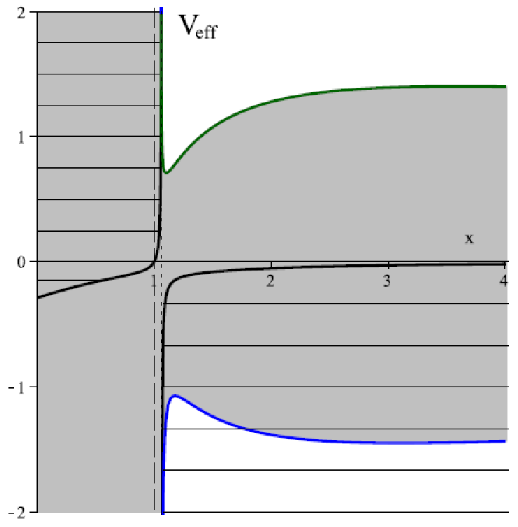
In the figs. 14, 15 and 16 the black solid line denotes the time potential (88). It presents the border of the dashed region. In the dashed regions for positive and negative values of energy the direction of time flow in (87) changes, i.e. becomes negative there. The grey region, as before, denotes the forbidden regions for motion.



IV Orbits
To visualize the geodesics we use the cartesian coordinates in the form:
| (89) |
where .
IV.1
We first consider motion in the plane . Then only motion w.r.t. the angle is present. From the function in the equation (18) follows that in this case and . This implies , and .
For the –equation (14) consists only of the –dependent part and a constant:
| (90) |
Next we carry out the same substitutions as in the section III.3. Integration of the equation (90) then yields
| (91) |
where as in the section III.3 , is given by (76) and for from the equation (73).
From the -equation (14) we observe that the left hand side vanishes at
| (92) |
This means that the angular direction of the test particle motion will be changed when arriving at this point. Such an effect is usually known to occur in the presence of an ergosphere as for example in the Kerr or Kerr-Newman spacetimes, where a counterrotating orbit will be forced to corotate with the black hole spacetime. But contrary to those spacetimes, the BMPV spacetime does not possess an ergoregion, since its horizon angular velocity vanishes. In the following we will call this surface the turnaround boundary.
In the following we show in the figs. 17, 18 and 19 two-dimensional plots for the underrotating case, .
The first three orbits in the figure 17 are many-world-bound orbits, and the orbit in the fourth figure is a two-world escape orbit. The orbits 17(a) and 17(b) correspond to the potential 2(a) with . The orbits 17(c) and 17(d) have opposite value. We see that in the plots 17(b), 17(c), 17(d) the orbits cross the dashed circle corresponding to the ‘turnaround boundary’, where the test particle changes its angular direction of motion. In the plot 17(a) the ‘turnaround boundary’ has no influence on the orbit.
In the figure 18 we show orbits for the same value of . In the fig. 18(a) the many-world-bound orbit is located inside the ‘turnaround boundary’ and the escape orbit 18(b)–outside. The two-world-escape orbit 18(c) experiences the influence of the ‘turnaround boundary’, similar to the orbit in the picture 17(d).
In the fig. 19 we show orbits for . The many-world bound orbits 19(a) and 19(c), plotted for different values of the energy , are angularly deflected at the ‘turnaround boundary’, while the escape orbits 19(b) and 19(d) remain far away from the ‘turnaround boundary’.


We now turn to orbits in the overrotating case, . In the figs. 20, 21 and 22 we show trajectories for and in the figs. 23 and 24 trajectories for and varying values of the separation constant or angular momentum . For there are bound and escape orbits possible as we know from the previous chapters.
In the figs. 20(a) and 20(c) bound orbits deflected at the ‘turnaround boundary’ are shown. The escape orbits 20(b) and 20(d) do not get influenced by the ‘turnaround boundary’. In the plot 21(a) a bound orbit is located inside the ‘turnaround boundary’, while the escape orbit 21(b) will be angularly deflected there. In the fig. 22(a) the bound orbit is behind the pseudo-horizon and lies beyond the ‘turnaround boundary’. The escape orbit 22(b) for the same value of energy is of general hyperbolic type.
The figs. 23(a) and 23(b) for show a bound orbit influenced by the ‘turnaround boundary’ and an escape orbit. In the orbit 24(a) a bound orbit in the form of a Christmas star is located inside the ‘turnaround boundary’, while the particle in the escape orbit 24(b) will change its angular direction of motion at the ‘turnaround boundary’.


IV.2 Three dimensional orbits
In this section we visualize three dimensional geodesics. The three dimensional orbits represent in this case a three-dimensional projection of the general four-dimensional orbits. This projection explains the sometimes not very smooth looking parts of the orbits in the figures below.
In the fig. 25 we show a many-world bound orbit 25(a) and an escape orbit 25(b) for the underrotating case with . Because of the choice of the coordinates there is a divergence at the horizon. The motion is continued on the inner side of the horizon.


In the fig. 26 we show trajectories for the overrotating case with . In the figs. 26(a) and 26(c) the orbits are bound and possess different values of the energy . In the fig. 26(c) the energy value is close to the minimum of the effective potential. Fig. 26(b) shows a corresponding escape orbit for the bound orbit 26(a), while the orbit 26(d) has an almost critical value of the energy corresponding to the maximum of the effective potential.


The trajectories in the fig. 27 are a bound orbit behind the pseudo-horizon 27(a) and an escape orbit 27(b) for the same value of the energy.


V Conclusions
In this paper we have discussed the orbits of neutral test particles in the BMPV spacetime. We have solved the full set of geodesic equations analytically in terms of the Weierstrass’ functions. We have analyzed in detail the effective potential of the radial equation, and presented a complete classification of the possible orbits in this spacetime. We have also addressed the causal properties of the BMPV spacetime. Our results are in full accordance with previous more qualitative discussions [2, 4, 5, 6].
- •
In the underrotating case, when the rotation parameter , the BMPV spacetime describes supersymmetric black holes. Here the velocity of light surface, which forms the boundary inside which causality violation can occur, is hidden behind the horizon, located at .
- •
In the overcritical case the BMPV spacetime represents in its exterior region a repulson. No geodesics can cross the pseudo-horizon located at . The exterior region is geodesically complete. The velocity of light surface is, however, outside the pseudo-horizon. Therefore this spacetime represents a naked time machine.
- •
In the critical case the surface has vanishing area and coincides with the velocity of light surface. As in the repulson case, no geodesics can cross this surface to reach the interior region . However, most types of orbits reach the surface .
To illustrate the analytical solutions we have presented various types of trajectories in the plane , and subsequently performed a three-dimensional projection for some selected orbits. An interesting effect present in many of the orbits is the change of the angular direction at the ‘turnaround boundary’, where the derivative of the azimuthal angle w.r.t. the radial coordinate vanishes. This effect arises although there is no ergosphere in the spacetime. The resulting orbits have rather intriguing shapes, differing from the ones of the Kerr, Kerr-Newman or Myers-Perry spacetimes.
In should be interesting to next address the motion of charged test particles in the BMPV spacetime. This should yield the full analytical solution of the set of equations presented and discussed by Herdeiro [4, 5]. An analogous analysis as the one given here should yield the complete classification of the possible types of orbits.
Since the BMPV solution may be considered as a subset of the more general family of solutions found by Chong, Cvetic, Lü and Pope [8], it will be interesting to extend the present study to this set of solutions. They include two unequal rotation parameters and describe also non-extremal solutions [8]. Moreover a cosmological constant is present. Particularly interesting should be the analysis of the included set of supersymmetric black holes and topological solitons.
Moreover, an extension of the present work to the intriguing set of solutions of gauged supergravities in four, five and seven dimensions, discussed by Cvetic, Gibbons, Lü and Pope [6], appears interesting. However, in analytical studies of the geodesics of such extended sets of solutions it may be necessary to employ more advanced mathematical tools based on hyperelliptic functions [19, 20, 21].
On the other hand, the BMPV spacetime can also be viewed as a special case of a more general family of solutions, where the Chern-Simons coupling constant, multiplying the term in the action, is a free parameter [3]. When this free parameter assumes a particular value, the BMPV solutions of minimal supergravity are obtained. For other values of this coupling constant new surprising phenomena occur. For instance, the resulting black hole solutions need no longer be uniquely specified in terms of their global charges [22] or an infinite sequence of extremal radially excited rotating black holes arises [23]. The study of the geodesics in these spacetime may also reveal some surprises.
Acknowledgments. We gratefully acknowledge discussions with Saskia Grunau, Burkhard Kleihaus and Eugen Radu, and support by the Deutsche Forschungsgemeinschaft (DFG), in particular, within the framework of the DFG Research Training group 1620 Models of gravity.
References
- [1] J. C. Breckenridge, R. C. Myers, A. W. Peet and C. Vafa, Phys. Lett. B 391, 93 (1997) [hep-th/9602065].
- [2] G. W. Gibbons and C. A. R. Herdeiro, Class. Quant. Grav. 16, 3619 (1999) [hep-th/9906098].
- [3] J. P. Gauntlett, R. C. Myers and P. K. Townsend, Class. Quant. Grav. 16, 1 (1999) [hep-th/9810204].
- [4] C. A. R. Herdeiro, Nucl. Phys. B 582, 363 (2000) [hep-th/0003063].
- [5] C. A. R. Herdeiro, Nucl. Phys. B 665, 189 (2003) [hep-th/0212002].
- [6] M. Cvetic, G. W. Gibbons, H. Lu and C. N. Pope, hep-th/0504080.
- [7] L. Dyson, JHEP 0701, 008 (2007) [hep-th/0608137].
- [8] Z. -W. Chong, M. Cvetic, H. Lu and C. N. Pope, Phys. Rev. Lett. 95, 161301 (2005) [hep-th/0506029].
- [9] C. W. Misner, K. S. Thorne, J. A. Wheeler, Gravitation, W.H. Freeman and Company, (San Francisco) (1973)
- [10] Y. Mino, Phys. Rev. D 67, 084027 (2003) [gr-qc/0302075].
- [11] A. I. Markushevich, Theory of functions of a complex variable, Vol. III, Prentice-Hall, Inc., Englewood Cliffs, N.J. (1967).
- [12] S. Grunau and V. Kagramanova, Phys. Rev. D 83, 044009 (2011) [arXiv:1011.5399 [gr-qc]].
- [13] E. Hackmann and H. Xu, Phys. Rev. D 87, 124030 (2013) [arXiv:1304.2142 [gr-qc]].
- [14] V. Kagramanova and S. Reimers, Phys. Rev. D 86, 084029 (2012) [arXiv:1208.3686 [gr-qc]].
- [15] B. O’Neil, The Geometry of Kerr Black Holes (A.K. Peters, Wellesley, MA, 1995).
- [16] V. Kagramanova, J. Kunz, E. Hackmann and C. Lämmerzahl, Phys. Rev. D 81, 124044 (2010) [arXiv:1002.4342 [gr-qc]].
- [17] E. Hackmann, C. Lämmerzahl, V. Kagramanova and J. Kunz, Phys. Rev. D 81, 044020 (2010) [arXiv:1009.6117 [gr-qc]].
- [18] S. Chandrasekhar, The Mathematical Theory of Black Holes (Oxford University Press, Oxford, 1983).
- [19] E. Hackmann and C. Lämmerzahl, Phys. Rev. Lett. 100, 171101 (2008).
- [20] E. Hackmann, V. Kagramanova, J. Kunz and C. Lämmerzahl, Phys. Rev. D 78, 124018 (2008) [Erratum-ibid. 79, 029901 (2009)] [arXiv:0812.2428 [gr-qc]].
- [21] V. Z. Enolski, E. Hackmann, V. Kagramanova, J. Kunz and C. Lammerzahl, J. Geom. Phys. 61, 899 (2011) [arXiv:1011.6459 [gr-qc]].
- [22] J. Kunz and F. Navarro-Lerida, Phys. Rev. Lett. 96, 081101 (2006) [hep-th/0510250].
- [23] J. L. Blazquez-Salcedo, J. Kunz, F. Navarro-Lerida and E. Radu, arXiv:1308.0548 [gr-qc].