The 14th case VHS via K3 fibrationsThanks: A. Clingher was supported by Simons Foundation grant no. 208258 and by a Bitdefender Invited Professor scholarship from IMARThanks: C. F. Doran and A. Y. Novoseltsev were supported by the Natural Sciences and Engineering Resource Council of Canada (NSERC), the Pacific Institute for the Mathematical Sciences, and the McCalla Professorship at the University of AlbertaThanks: J. Lewis was supported in part by NSF grant OISE-0965183Thanks: A. Thompson was supported in part by NSERC and in part by a Fields Institute Ontario Postdoctoral Fellowship with funding provided by NSERC and the Ontario Ministry of Training, Colleges
and Universities
Date: August 24, 2026
Abstract.
We present a study of certain singular one-parameter subfamilies of Calabi-Yau threefolds realized as anticanonical hypersurfaces or complete intersections in toric varieties. Our attention to these families is motivated by the Doran-Morgan classification of variations of Hodge structure which can underlie families of Calabi-Yau threefolds with over the thrice-punctured sphere. We explore their torically induced fibrations by -polarized K3 surfaces and use these fibrations to construct an explicit geometric transition between an anticanonical hypersurface and a nef complete intersection through a singular subfamily of hypersurfaces. Moreover, we show that another singular subfamily provides a geometric realization of the missing “14th case” variation of Hodge structure from the Doran-Morgan list.
1. Introduction
In their paper [DM06], Doran and Morgan give a classification of the possible variations of Hodge structure that can underlie families of Calabi-Yau threefolds with over the thrice-punctured sphere. They find fourteen possibilities. At the time of publication of [DM06], explicit families of Calabi-Yau threefolds realising thirteen of these cases were known and are given in [DM06, Table 1]. The aim of this paper is to give a geometric example which realizes the fourteenth and final case (henceforth known as the 14th case) from their classification, and to study its properties.
By analogy with other examples (see [DM06, Section 4.2]), one might expect that the 14th case variation of Hodge structure should be realized by the mirror of a complete intersection of bidegree in the weighted projective space . However, this ambient space is not Fano, so the Batyrev-Borisov mirror construction cannot be applied to obtain such a mirror family.
Instead, Kreuzer and Sheidegger [KKRS05] suggest working with a slightly different ambient space, given by a non-crepant blow up of . However, the complete intersection Calabi-Yau threefold of bidegree in this ambient space has , so its mirror will have , making it unsuitable as a candidate for the 14th case on the Doran-Morgan list.
We take as the starting point for our discussion this mirror family with , which we denote by . We begin by constructing it explicitly and exploring its properties, noting that it has a singular one-parameter subfamily with GKZ series matching that predicted for the 14th case. Moreover, we find that has a torically induced fibration by K3 surfaces given as anticanonical hypersurfaces in the three-dimensional space polar to .
The existence of this fibration suggests that a model for the 14th case variation of Hodge structure could also be constructed by considering Calabi-Yau threefolds admitting fibrations by anticanonical hypersurfaces in the space polar to . A computer search for such fibrations yields a second candidate family, , which is mirror to a hypersurface of degree in the weighted projective space . The threefolds in this family also have .
This poses the natural question of whether the two families and are related. A careful study of the geometry of each shows that the generic fibre of their K3 fibrations is polarized by the lattice . Lattice polarized K3 surfaces of this type were studied by [CD07] and [CDLW09]; using their results we are able to show that the K3 fibrations on and are very closely related. With this relationship as a guide, we proceed to find an explicit geometric transition between the two, by degenerating to a singular subfamily and blowing up to obtain .
Having shown that the families and are in fact two halves of the same picture, we turn our focus back to the family and, in particular, its singular subfamily . The main results of this paper are Lemma 6.1 and Theorem 6.4, which describe the mixed Hodge structure on the cohomology groups of . Together they imply:
Theorem 1.1.
The mixed Hodge structure on the cohomology groups is pure unless and the weight filtration on has the following description:
Furthermore, as varies in its one-parameter subfamily, the third graded piece admits a pure variation of Hodge structure of weight and type , which realizes the 14th case variation of Hodge structure.
A crucial step in the proof of this theorem involves quotienting the threefold by a certain involution and resolving to obtain a new family of Calabi-Yau threefolds . This new family is closely related to and is interesting in its own right. The K3 fibration on induces a fibration of by Kummer surfaces, via the mechanism discussed in [CD07]. We digress to show how may be constructed directly as a family of Kummer surfaces using the techniques of [DHNT13]; this provides a great deal of insight into the geometry of this new threefold.
Finally, we conclude by discussing the mirrors of the families and considered here, and compute a mirror for the geometric transition between them. In particular, we find that the singular subfamily may naturally be seen as the mirror of a complete intersection of bidegree in , as originally expected. We note, however, that does not admit a Calabi-Yau resolution, despite the fact that its mirror admits a Calabi-Yau smoothing. This provides a counterexample to a conjecture of Morrison [Mor99].
The structure of this paper is as follows. In 2, we give an overview of relevant results from toric geometry that will be used throughout the rest of the paper; this also serves the function of setting up the notation that will be used in what follows. Then in 3 we construct the families and and study some of their basic properties, these are summarized by Propositions 3.1 and 3.2. In particular, Proposition 3.1 shows that has a subfamily with GKZ series matching that predicted for the 14th case variation of Hodge structure.
We begin 4 with a detailed study of the K3 fibrations on and , using results of [CD07] and [CDLW09]. From this, we show that the parameters describing the K3 fibration on match with those describing the K3 fibration on a certain subfamily of , and those describing the K3 fibration on the subfamily match with those describing the K3 fibration on a further subfamily of . These subfamilies , and of and are studied in 5; their properties are summarized by Propositions 5.1 and 5.2. Using these results, we show in Proposition 5.3 that the families and are in fact related by a geometric transition, through the subfamily , and that this transition also relates the subfamilies and .
6 begins with a result, Lemma 6.1, which describes the mixed Hodge structure on the cohomology groups of the subfamily . However, there is an ambiguity in the description of the weight filtration on given by this lemma, which prevents us from drawing any conclusions. To resolve this, we study the action of certain involutions on , which restrict to the subfamily . The resolved quotient of by one such involution gives a new Calabi-Yau threefold, , with geometry closely related to that of . Proposition 6.2 and Corollary 6.3 describe this geometry; from them we are able to deduce Theorem 6.4 and Corollary 6.5, which complete the description of the subfamily . In particular, we find that realizes the 14th case variation of Hodge structure that we have been seeking.
In 7 we digress to discuss the geometry of the Calabi-Yau threefolds . The K3 fibration on induces a K3 fibration on , the general fibre of which is a Kummer surface. We use this K3 fibration, along with the methods of [DHNT13], to construct a model for directly. The geometric nature of this construction provides a great deal of insight into the geometry of and demonstrates the utility of the methods of [DHNT13] in a practical example.
Finally, in 8 we compute mirrors for and , their subfamilies , and , and exhibit a mirror for the geometric transition between them. In particular, we find that may be seen as a mirror to a complete intersection of degree in , as expected. Finally, we show that and its mirror provide a counterexample to a conjecture of Morrison [Mor99].
Most of the computer-aided computations performed for this work were done in the free open source mathematics software Sage [S+15], specifically using the toric geometry framework developed by Braun and Novoseltsev [BN12]. At the time of this writing, it is necessary to use a small extra patch11
1
Available as a git branch at https://github.com/novoselt/sage/commits/Cayley, but we plan to integrate it into the official release of Sage. An interested reader may easily reproduce all computations used in this article following the presented code, as well as adjust them to suit his or her own needs. Typesetting of code snippets and some of the complicated expressions was greatly facilitated by SageTeX [D+12].
1.1. Acknowledgements
The authors would like to thank Andrew Harder and Ursula Whitcher for their assistance with some of the calculations in 7. A. Clingher would like to thank the Institute of Mathematics “Simion Stoilow” of the Romanian Academy in Bucharest, the Institut des Hautes Études Scientifique in Bures-sur-Yvette and the Max Planck Institute for Mathematics in Bonn for their hospitality and support during the academic year 2012-2013. A portion of this work was completed while A. Thompson was in residence at the Fields Institute Thematic Program on Calabi-Yau Varieties: Arithmetic, Geometry and Physics; he would like to thank the Fields Institute for their support and hospitality.
2. Toric Geometry Review and Notation
In this section we recall the basic facts of toric geometry in order to set up notation that will be used in the rest of the paper; we refer to the wonderful book [CLS11] for details. We also briefly describe Batyrev’s construction of mirror families of Calabi-Yau anticanonical hypersurfaces in toric varieties [Bat94] and its generalization to nef complete intersections by Batyrev and Borisov [BB96b]. We conclude with a discussion of fibrations of Calabi-Yau varieties that can be obtained from natural fibrations of their ambient spaces.
2.1. Toric Varieties
Let and be dual lattices of rank , i.e. as free Abelian groups, where is identified with and with using the natural pairing . The real vector space associated to a lattice will be denoted by the subscript , e.g. the real vector space associated to the lattice is The torus of a lattice is defined to be , it is an affine variety with group structure corresponding to componentwise multiplication in and character lattice .
A cone will always be convex, polyhedral, and rational. Its dual cone will be denoted by . The affine toric variety corresponding to a cone will be denoted by .
For a fan in , we will denote by the corresponding toric variety and by the set of its -dimensional cones. In particular, is the set of rays and for each ray we have a primitive integral generator , a homogeneous coordinate , and a prime torus-invariant Weil divisor given by .
Any toric divisor has an associated polyhedron given by
For any , the -homogenization of the character is the monomial
and the global sections of are
Of particular interest to us are the toric canonical divisor and the global sections of the anticanonical divisor, in the following special case.
2.2. Gorenstein Fano Toric Varieties
Gorenstein Fano toric varieties are in bijection (after taking into account equivalences) with reflexive polytopes. A reflexive polytope is a full-dimensional lattice polytope that contains the origin in its interior and has polar
that is also a lattice polytope. Since , there is a polar duality between reflexive polytopes in and reflexive polytopes in , and even an inclusion-reversing bijective correspondence between the faces of and .
Given a reflexive polytope , its normal fan in will be denoted by . To avoid towers of subscripts, we will simply write instead of for the toric variety associated to this fan. The vertices of coincide with the primitive integral generators of rays of , so one can also think of as the face fan of (with cones over faces of ).
Definition 2.1.
Let be a reflexive polytope and let be a subdivision of . If all rays of are generated by (some of) the boundary lattice points of , it is a crepant subdivision. If is also simplicial and the corresponding toric variety is projective, it is a projective crepant subdivision. If furthermore all boundary lattice points of generate rays of , it is a maximal projective crepant subdivision.
Such subdivisions correspond to maximal projective crepant partial desingularizations (MPCP-desingularizations), introduced by Batyrev in [Bat94]. They lead to a very concrete construction of Calabi-Yau orbifolds.
Theorem 2.2.
Let be a reflexive polytope of dimension . A generic anticanonical hypersurface in , i.e. a generic section , is a Calabi-Yau variety of dimension . A generic anticanonical hypersurface in , where is a projective crepant subdivision of , is a Calabi-Yau orbifold of dimension .
Proof.
See [CK99, Proposition 4.1.3].
∎
For a reflexive polytope , projective crepant subdivisions of correspond to special triangulations of the boundary of . For any such subdivision the polytope of the anticanonical divisor is easily seen to be itself. This means that in the equations of the anticanonical Calabi-Yau hypersurfaces, the variables correspond to lattice points of while the (coefficients of) monomials correspond to lattice points of :
Polar duality of reflexive polytopes means that the roles of and in the above discussion can be reversed, leading to another family of hypersurfaces in another toric variety. Batyrev showed [Bat94] that if , then generic anticanonical hypersurfaces in MPCP-desingularizations of are smooth Calabi-Yau threefolds and the exchange corresponds to the exchange of the Hodge numbers of the anticanonical hypersurfaces of the two families, making them candidates for mirror pairs.
2.3. Nef Complete Intersections
Batyrev and Borisov generalized the construction of Calabi-Yau varieties as anticanonical hypersurfaces in toric varieties to the case of complete intersections associated to nef-partitions of reflexive polytopes [Bor93, BB96b].
Definition 2.3.
Let be a reflexive polytope. A nef-partition is a decomposition of the vertex set of into a disjoint union
such that all divisors are Cartier. Equivalently, let be the convex hull of the vertices from and the origin. These polytopes form a nef-partition if their Minkowski sum is a reflexive polytope.
The dual nef-partition is formed by the polytopes of the , which give a decomposition of the vertex set of ; their Minkowski sum is .
“Nef-partition” may refer to any of the following decompositions:
- 1)
into a disjoint union of ,
- 2)
into a Minkowski sum of ,
- 3)
the anticanonical divisor of into a sum of .
Each of these decompositions can be easily translated into the others. Some care should be taken only to avoid mixing a nef-partition and its dual.
It follows from the definition that polar duality of reflexive polytopes switches convex hull and Minkowski sum for dual nef-partitions:
Given a nef-partition of an -dimensional reflexive polytope consisting of -parts, generic sections of the divisors determine an -dimensional complete intersection Calabi-Yau variety. In [BB96a] Batyrev and Borisov show that such varieties corresponding to dual nef-partitions have mirror-symmetric stringy Hodge numbers, which we will denote by .
2.4. Torically Induced Fibrations
Let and be lattices, be a fan in , and be a fan in . There is a bijection between toric morphisms (i.e. morphisms of toric varieties preserving the group structure of their tori) and fan morphisms (i.e. lattice homomorphisms compatible with the fan structure: the linear extension of maps each cone into a single cone ).
Consider the special case when the lattice homomorphism is surjective, i.e. we have an exact sequence of lattices
where . Let . We can consider either as a fan in or as a fan in , giving two corresponding toric varieties (a dense subset of ) and .
As discussed in [CLS11, § 3.3], there is a clear relation between these two varieties,
In fact , so part of is a fibre bundle over , with fibres . Moreover, if is split by and , then the whole of is a fibre bundle over (see [CLS11, Definition 3.3.18 and Theorem 3.3.19]). However, splitting is a very strong condition on fans, so instead of imposing it we will work with more general fibrations than fibre bundles.
Definition 2.4.
Let be a morphism between two varieties. Then is a fibration if it is surjective and all of its fibres have the same dimension .
In [HLY02, Proposition 2.1.4] the authors provide a detailed description of the fibres of arbitrary toric morphisms22
2
Note that while the notation in [HLY02] is very similar to ours, the authors sometimes implicitly assume that toric varieties in question are complete.. However, we are primarily interested in fibrations , as they may induce fibrations of Calabi-Yau subvarieties realized as anticanonical hypersurfaces or nef complete intersections in . This fibration condition may prevent from being “too refined”, leading to singularities of , but it may still be possible to compose with a crepant resolution of singularities in such a way that becomes smooth and the restriction of the composition to is still a fibration.
We now describe a strategy for searching for such toric fibrations. Let be a reflexive polytope and let be a crepant subdivision of . Suppose that is a fibration (meaning that is a fibration in the above sense). As before, its fibre is determined by the subfan of in the sublattice of . Since we would like the fibres of Calabi-Yau subvarieties to be lower-dimensional Calabi-Yau varieties, it is natural to require that is also associated to a reflexive polytope, i.e. that it is a crepant subdivision of for some , where is the dual lattice of . In this case is a “slice” of by a linear subspace, so one can search for such slices of and take to be the projection along the linear subspace of .
We can also reformulate this problem in dual terms: and the condition that is inside implies that the image of in is inside . So alternatively one can look for “projections” of that are reflexive. Here we recall that the origin is the only interior lattice point of any reflexive polytope, so all lattice points of must be projected onto either the origin or the boundary of the projection. Due to this restriction a “large” with many lattice points is less likely to have any fibrations than a “small” one.
3. Models
3.1. Complete Intersections
In [DM06] Doran and Morgan have shown that there are 14 possible classes of variations of Hodge structure which can be associated to families of Calabi-Yau threefolds with . They have provided explicit examples for all but one of these classes and given some suggestions on how one could construct an example for the last class (the “14th case” referred to in the title of this paper).
By analogy with other examples, one could hope to start with a complete intersection with in the weighted projective space . Unfortunately this ambient space is not Fano, so the Batyrev-Borisov mirror construction based on nef-partitions, described in 2.3, cannot be applied to obtain a family with . Instead, Kreuzer and Sheidegger have suggested working with a slightly different ambient space, a non-crepant blow-up of , which is Fano and has a family of complete intersections corresponding to a suitable nef-partition, so the mirror transition is possible (See [KKRS05, Section 8 and Appendix E.2] for some discussion of this example). We will construct and explore this mirror family below using Sage.
Let be a -dimensional reflexive polytope with polar given by
i.e. the vertices of are given by the columns of the following matrix
(3.1)
The nef-partition we are interested in is “in agreement” with the block structure of this matrix: one part is formed by the first four vertices and the other by the last six.
Let be a crepant subdivision of and be the corresponding crepant partial resolution of . The choice of this resolution will depend on our needs, but for the moment we only ensure that is simplicial. We will use to denote homogeneous coordinates on , with being the index of the corresponding point of . For future use we also introduce parameters , , and into the base field of . Finally, we let be a generic member of the family of complete intersections corresponding to the nef-partition above.
The defining polynomials of are
(3.2)
(3.3)
There are 12 parameters in these equations, but their number can be significantly reduced. First of all, we can use a change of variables to set . To see this more easily, we switch to an affine chart.
In this chart takes the form
and making a substitution , does not lead to any new monomials.
From this we see that one can pick , , and to make the coefficients of the 3 monomials , and vanish, leaving only 9 parameters. Since we can also scale both polynomials and 5 of the variables, we can further reduce the number of parameters to 2.
On the other hand, computing stringy Hodge numbers of (one can use the generating function from [BB96a] implemented in PALP [KS04] or the closed form expressions from [DN10]) we obtain
If we take to be a MPCP-desingularization of , then is generically smooth and its stringy Hodge numbers coincide with its regular ones, so the dimension of the space of complex deformations of is . The fact that we have reduced the number of parameters in the defining polynomials of to suggests that the dimension of the space of polynomial deformations of is . To confirm this observation we compute the toric part of for the Batyrev-Borisov mirror of inside a MPCP-desingularization of (it is easier to work with a maximal resolution in this case, since is much smaller than , i.e. it has only a few lattice points.)
Here we have restricted the monomials used in the defining equations of to save some time, since the nef divisors corresponding to it have hundreds of monomial sections and we only need its cohomology class. Note that is smooth, so is (generically) smooth as well, giving . To compute (the contribution of to ), we just need to consider the intersections of the cohomology class of with the generators of the cohomology ring of . As can be seen from the above output, this ring can be generated by the last five of “all generators”, each of which corresponds to a torus-invariant subvariety of codimension , e.g. [z5] corresponds to , whose cohomology class is equivalent to , , and .
From this we conclude that .
As pointed out in [DM06], a certain subfamily of the complete intersections has the desired hypergeometric series corresponding to the 14th case. To describe that subfamily precisely in our setting we will compute the GKZ series of , following the algorithm outlined in [CK99, Section 5.5] and [KKRS05, Appendix A].
It is easy to check that the monomials that can be eliminated in the equations for correspond to all points of that are neither vertices of nor the origin (whilst this is true for our particular case, in general such information cannot be easily determined and one has to perform computations in the cohomology ring as above). Let’s use this information to reconstruct our varieties:
We now use the generators of the Mori cone of to construct moduli parameters of . These generators are given as elements of the row span of the Gale transform of the fan of , the -th element of each generator corresponds to the -th ray of this fan, except for the last one which corresponds to the origin and is equal to the negative sum of other entries. Note that for complete intersections we need to take such sums for each part of the nef-partition separately; the following code adds them in a way that is compatible with the order of coefficients of in Sage, with and corresponding to the origin (the coefficient-monomial correspondence for the newly constructed is the same as in (3.2) and (3.3), since the coefficient indices come from the internal enumeration of polytope lattice points).
We find that the modular parameters of are
and its GKZ series is
where the summation is over all integers and such that the arguments of all factorials are non-negative. Making a substitution , we can sum over all non-negative integers:
To simplify the description of further, we now scale its defining polynomials and coordinates to set all coefficients to except for and .
The defining polynomials of become
(3.4)
(3.5)
and the GKZ series takes the form
Comparing this series with the one given in the end of [DM06], we see that the subfamily of interest is , leading to the series
This subfamily, henceforth denoted by , will be of further interest in our pursuit of a geometric model for the 14th case; we will come back to it in 5.2.
We complete this subsection by showing that the complete intersections admit a natural fibration structure, which will allow us to access many of their properties. Going back to the definition of in (3.1), we observe that, in addition to its column decomposition into a nef-partition, it has a “natural” row decomposition. Indeed, the projection onto the first two coordinates corresponds to a toric fibration over a -dimensional toric variety , as long as we pick a compatible resolution of . To get such a resolution, we start with the face fan of , take its minimal subdivision compatible with the projection, and then subdivide it to get a simplicial fan, so that is an orbifold.
In homogeneous coordinates
Note that the hypersurface defined by the polynomial in (3.4) depends only on the variables involved in the projection map. This means that we can interpret as a defining equation of a curve and as a defining equation of a surface in each fibre of , in other words, induces a fibration of the complete intersection over .
Generic fibres of correspond to the fan whose rays are generated by the last four vertices of . The polytope spanned by these vertices is the last (the 4318-th) -dimensional reflexive polytope in the Kreuzer-Skarke list (included in Sage), with its normal fan corresponding to :
Summarizing the results of this section, we find:
Proposition 3.1.
The complete intersection model is generically a smooth Calabi-Yau threefold having and . There is a torically induced fibration onto a curve whose generic fibre is an anticanonical hypersurface in the three-dimensional space polar to .
Furthermore, the GKZ series of the subfamily obtained by setting the modular parameter coincides with the GKZ series predicted for the 14th case VHS.
3.2. Anticanonical Hypersurfaces
In the previous section we were able to represent the complete intersection as a fibration over a curve with fibres living in the space polar to . This suggests that the 14th case could also be realized by a family of anticanonical hypersurfaces in a four-dimensional space which can be fibred by the same toric varieties.
To try to find such a family, we searched33
3
We performed this search using Sage, but have chosen not to include the corresponding code in the text due to its length. The algorithm used simply runs over all hyperplanes that intersect a given polytope in a sublattice polytope, with a few technical tricks to make this search happen in a reasonable timeframe and to store the results of big searches compactly. The interested reader may find a Sage worksheet implementing this search attached to the arXiv submission of this paper (note, however, that in order to run this worksheet it is necessary to install the optional package polytopes_db_4d; beware of the 8.7GB download size!) for Fano varieties fibred by the space polar to among those whose anticanonical hypersurfaces have small , with the extra condition that the torically induced fibration is “balanced”: this means that the same 3-dimensional reflexive polytopes can play the roles of both slices and projections, as described in 2.4. The space polar to satisfies these requirements; below we study the family of anticanonical hypersurfaces in it.
Let be a -dimensional reflexive polytope given by
i.e. the vertices of and of are given by columns of the following matrices
Let be a crepant subdivision of and be the corresponding crepant partial resolution of . As before the choice of this resolution will depend on our needs; for now we add only one extra ray in addition to the vertices of , specifically the ray corresponding to the midpoint between the -th and the -rd vertices, which is the -th point in the internal enumeration in Sage:
This extra ray is necessary to make compatible with the projection onto the line in the direction . If with coordinates corresponding to the (unique) complete fan on this line and is the toric morphism associated to this projection, then
(3.6)
Let be a generic anticanonical hypersurface. Its defining polynomial is
Scaling the whole polynomial and four independent coordinates we can eliminate 5 out of 8 parameters. Using Batyrev’s formulas for the Hodge numbers of anticanonical hypersurfaces we check that , so we should indeed have 3 independent parameters. Summarizing, we find:
Proposition 3.2.
The hypersurface model is generically a smooth Calabi-Yau threefold with . There is a torically induced fibration whose general fibre is an anticanonical hypersurface in the three-dimensional space polar to .
Anticanonical hypersurfaces inside the space polar to were extensively studied by Billó et al. [BDF+98]; in order to conveniently use their results we will match our toric description with theirs (they considered hypersurfaces in with extra symmetries, which allow taking the quotient under a certain group action).
First, we rewrite the polynomial of in its “fibred” form, thinking of it as a polynomial in only and working in a chart with :
Now we can compare our representation with equation (4.19) in [BDF+98]:
We see that the matching of coordinates and coefficients is
and
To match these remaining parameters we use the definition of given by equation (3.18) in [BDF+98]:
where is an affine coordinate on the base of the fibration, so
We can use these parameters in Sage as follows:
Now the defining polynomial of has the form
One of the four parameters in this representation is redundant, e.g. we can set .
3.3. Geometric Transitions
Both the complete intersections and anticanonical hypersurfaces presented above have , while the original goal in their construction was to obtain families with that could provide geometric examples of the 14th case. In fact, in the hypersurface case it was known in advance that we would “fail”, since it is known that there are only 5 reflexive polytopes yielding Calabi-Yau threefolds with and [DM06] showed that they already provide examples for other classes of Hodge structure variations.
However, we can still try to obtain our desired families by using subfamilies of the constructed ones. Of course, simply fixing some of the parameters does not change the Hodge numbers of the Calabi-Yau threefolds in question, but if these threefolds were to become singular we could try to resolve the singularities and hope that holds for the resolved family. So we are now looking for geometric transitions from the already constructed families to some new ones with, hopefully, “correct” Hodge numbers.
The existence of such geometric transitions was first suggested by Clemens [Cle83a, Cle83b] and later expanded upon by Friedman [Fri86]. In this subsection we give a precise definition and a basic classification of geometric transitions, following [Ros11].
Definition 3.3.
Let and be smooth Calabi-Yau threefolds. They are connected by a geometric transition if there exist a normal variety , a birational contraction , and a complex deformation (smoothing) of to .
It is a primitive geometric transition if cannot be factored into birational morphisms of normal varieties.
It is a conifold transition if has only conifold singularities (ordinary double points).
It is a trivial geometric transition if is a deformation of .
Theorem 3.4.
Let be a primitive contraction of a smooth Calabi-Yau threefold to a normal variety . Let be the exceptional locus of . Then is of one of the following three types:
- Type I
is small, may be reducible and is composed of finitely many rational curves;
- Type II
contracts a divisor to a point, is irreducible and is a generalized del Pezzo surface;
- Type III
contracts a divisor to a smooth curve , is irreducible and is a conic bundle over .
Definition 3.5.
A primitive geometric transition is of type I, II, or III, if the corresponding birational contraction is of type I, II, or III, respectively.
The existence of geometric transitions relating Calabi-Yau threefolds with different Hodge numbers has interesting consequences for their moduli spaces. In particular, it has been suggested [Rei87, Fri91] that geometric transitions could be used to connect together the moduli spaces of all compact complex threefolds with trivial canonical bundle. Moreover, it is also natural to ask how geometric transitions interact with the string-theoretic phenomenon of mirror symmetry [Dix88, CLS90, GP90] and this has been the object of a great deal of study; a good summary of this theory is given by Morrison [Mor99]. We will return to the question of mirror symmetry in our context in 8.
However, before we use geometric transitions to construct new families, we first find that our two models and are in fact connected via a type III geometric transition. To see this explicitly, we begin by comparing their fibration structures.
4. Matching the Models
4.1. K3 Fibrations
The generic fibres of the fibrations induced by and constructed earlier are anticanonical hypersurfaces inside the three-dimensional space polar to , i.e. they are generically two-dimensional Calabi-Yau varieties: K3 surfaces. The choice of toric ambient space for them induces a lattice polarization, in this case by the lattice , where is the hyperbolic lattice of rank and is the unique even negative-definite unimodular lattice of rank . Such -polarized K3 surfaces (the name “-polarized” is a bit unfortunate in the toric context, but it should not cause too much confusion) were originally studied by Shioda and Inose [SI77, Ino78] and have recently been revisited in [Shi06], [CD07] and [CDLW09], we start this section with a summary of their properties.
Definition 4.1.
An -polarization on a K3 surface is a primitive lattice embedding , such that the image in the Néron-Severi lattice contains a pseudo-ample class (corresponding to an effective nef divisor with positive self-intersection).
Definition 4.2.
Let be a K3 surface. An involution on is a Nikulin involution if for any holomorphic 2-form on .
Theorem 4.3.
Let be an -polarized K3 surface. Then
- 1)
is isomorphic to the minimal resolution of a quartic surface in given by
- 2)
the parameters , , and in the above equation specify a unique point with ;
- 3)
canonically corresponds to a pair of elliptic curves ;
- 4)
the modular parameters of and are related by
- 5)
generically there are exactly two isomorphism classes of elliptic fibrations with section on : the “standard” fibration, which has an polarization realized via two type exceptional fibres, and the “alternate” fibration which has an polarization realized via a type exceptional fibre;
- 6)
there exists a Nikulin involution on .
Proof.
Proposition 4.4.
An anticanonical hypersurface in the space polar to the weighted projective is an -polarized K3 surface defined by
It is related to the normal form given in Theorem 4.3 by
Proof.
Both the standard and alternate elliptic fibrations have toric realizations on the anticanonical hypersurfaces in the above proposition. Here we will point out a few key facts about this toric picture that will be used later; for a detailed treatment of the combinatorics of torically induced elliptic fibrations of K3 surfaces we refer the reader to [PS97] or [Roh04].
In our case the toric correction term is zero, meaning that the intersection pattern of divisors on a generic anticanonical hypersurface, which have three linear relations between them, is given by the -skeleton of the reflexive polytope in the lattice . Two directions in determine the two fibrations over , and the ADE diagrams of the fibres over zero and infinity are given by the parts of the -skeleton that are projected into the interiors of rays of the fan. Here is an explicit construction of these diagrams:
The graphs constructed above are shown in 1–3. In these graphs, the labels correspond to the indices of lattice points of the polytope P. For the standard fibration the toric divisor corresponding to point gives a uniquely defined section, and for the alternate fibration there are two toric sections corresponding to points and .
Figure 1. Intersection of toric divisors on an -polarized K3 surface.
Figure 2. ADE diagram of the standard fibration on an -polarized K3 surface.
Figure 3. ADE diagram of the alternate fibration on an -polarized K3 surface.
Next we will see how this theory can be applied to our models and . For the complete intersection model described in 3.1 the role of in Proposition 4.4 is played by . Using this we obtain the following expressions for the modular parameters of a fibre:
For the anticanonical hypersurface model from 3.2, correspond to and we compute
Next we switch to coordinates on the bases and of the fibrations and respectively:55
5
We have used the same notation , , , and in 3.1 and 3.2 to refer to different objects. When we need to consider them together and it is necessary to distinguish them, we will use their dimensions as superscripts. Names in Sage examples always include these dimensions to allow reusing of objects in later sections.
(4.1)
(4.2)
Finally, recall that is fibred not over , but over a curve corresponding to . It is easy to see from (3.4), that is the pullback of
(4.3)
Using the fan of , shown in 4, we can see that does not intersect the divisors corresponding to and , e.g. if then , since there are no cones containing rays corresponding to and or .
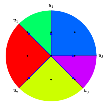 Figure 4. Base of the fibration
This means that is isomorphic to the curve in with coordinates , given by , i.e. with coordinates .
In terms of these new coordinates the modular parameters of a fibre are
(4.4)
(4.5)
Comparing expressions for and for the complete intersection model , (4.4) and (4.5), with analogous expressions for the anticanonical hypersurface model , (4.1) and (4.2), we see that they are quite similar. This similarity is even more striking if we let in (4.1) and (4.2), to obtain:
(4.6)
(4.7)
In fact, the expressions (4.4) and (4.5) and the expressions (4.6) and (4.7) would be exactly the same if we let and
(4.8)
Finally, we note also that with respect to the fibre modular parameters and , the subfamily of complete intersections with is very special: in this case , so all K3 fibres correspond to “complementary” elliptic curves with .
Figure 4. Base of the fibration
This means that is isomorphic to the curve in with coordinates , given by , i.e. with coordinates .
In terms of these new coordinates the modular parameters of a fibre are
(4.4)
(4.5)
Comparing expressions for and for the complete intersection model , (4.4) and (4.5), with analogous expressions for the anticanonical hypersurface model , (4.1) and (4.2), we see that they are quite similar. This similarity is even more striking if we let in (4.1) and (4.2), to obtain:
(4.6)
(4.7)
In fact, the expressions (4.4) and (4.5) and the expressions (4.6) and (4.7) would be exactly the same if we let and
(4.8)
Finally, we note also that with respect to the fibre modular parameters and , the subfamily of complete intersections with is very special: in this case , so all K3 fibres correspond to “complementary” elliptic curves with .
4.2. Ambient Space Morphism
Given such a perfect matching of modular parameters, we may try to construct a morphism between the original varieties , perhaps by constructing a morphism (ideally, a fibration) between their ambient spaces . Combining all correspondences used so far, we get
or, more concretely,
This correspondence does not give us a morphism between toric varieties, since only some of the homogeneous coordinates on are used and they are unlikely to be well-defined due to relations involving the other coordinates. But we may look for a fan morphism that will at least map the rays corresponding to these selected to the rays corresponding to the indicated .
This computation shows that if such a fan morphism exists, it must be given by the matrix m
which is unique since m_y has maximal rank. If this matrix defines a fibration, then rays of must be mapped onto rays of or the origin.
Since all necessary image rays can be generated by lattice points of , we can pick to be a crepant subdivision of . One can then subdivide the current (the subdivision of compatible with the fibration ) to obtain a fibration over , but, unfortunately, this subdivision of will not be crepant.
To fix this problem, we go back to the defining polynomial (4.3) of the curve and the fan of , shown in 4. We have already established that does not intersect the divisors corresponding to and . Now we note that it also does not contain the point with , since this would imply that one of the other coordinates is zero, which is not possible. This means that is completely contained within the part of corresponding to the fan generated by the rays of , , and . But then is completely contained within the toric variety corresponding to without all cones that contain rays corresponding to either , or , or and together. Starting with such a subfan of , we can find a subdivision that leads to a fibration with affine lines as generic fibres.
Now not only can all necessary rays in the codomain be generated by lattice points of , but also all necessary rays in the domain can be generated by lattice points of . We can therefore think of as an open subset in some crepant partial desingularization of , whilst is still a Calabi-Yau variety.
From the computational point of view, we can no longer use the framework of CPR-Fano toric varieties in Sage to represent ; instead we have to use generic toric varieties. We will however still use the same convention for naming coordinates: the missing and now reflect the fact that we are interested only in charts where they are non-zero, in which case both can be set to using relations between coordinates.
In homogeneous coordinates we get
which also does not involve , since it corresponds to the only ray of the kernel fan. This map can be used to pull back and compare it with . We delay this comparison, however, since for analysis of singularities it is convenient to perform a few more subdivisions of the underlying fans first.
5. Singular Subfamilies
5.1. Hypersurfaces
Generically, complete intersections and anticanonical hypersurfaces in MPCP-desingularizations of their ambient spaces are smooth, since the singular locus in this case has codimension at least four. However, in this paper we are also interested in the following subfamilies:
1)
complete intersections with , corresponding to the subfamily with the desired GKZ series, we will denote a generic member of this subfamily as to emphasize dependence on a single parameter only;
2)
hypersurfaces with , corresponding to the subfamily whose K3 fibration can be “perfectly matched” with the K3 fibration of complete intersections , we will denote a generic member of this subfamily as ;
3)
hypersurfaces with and , corresponding to the subfamily of the above subfamily with an analogue of the restriction, we will denote a generic member of this subfamily as .
Generic members of these subfamilies may be singular, we analyze their singularities using results of [BDF+98] and computer software (Sage interfacing with Magma [BCP97] for computing the singular loci of affine varieties). We begin in this subsection with an analysis of the singularities of the hypersurfaces and .
The singular locus in the moduli space of hypersurfaces is summarized in relations (4.39) of [BDF+98]:
Here relations and are actually the same, in the sense that they are switched by an appropriate change of coordinates (there is a finite group action on the simplified polynomial moduli space of hypersurfaces). We see that the hypersurfaces are singular (and, therefore, cannot be isomorphic to the full two-parameter family of complete intersections ), since the condition is satisfied. The condition makes relations and the same, but does not impose singularities on its own.
An explicit chart-by-chart check for singularities of using our current fan and ignoring the orbifold structure of (i.e. ignoring singularities of which are inevitable due to the ambient space structure) reveals a singular locus of dimension 1 in all charts involving . To study this singular locus, it is convenient to put it into smooth charts of ; in order to do this we need to subdivide further.
In fact, when doing this one finds that it is better to start afresh with . Recall that adding the ray corresponding to the 16-th point of , which is the midpoint between the vertices and , was necessary to ensure compatibility with the fibration . We also had to add to allow for a fibration . This is the only interior point of the triangular face on , , and . The face fan of this triangle (in the spanned affine sublattice with being the origin) is the fan of , and the three interior points of its edges correspond to , , and . Adding all these rays is sufficient to resolve all singularities of the 3-dimensional cone on , , and , but the resulting subcones are still faces of singular 4-dimensional cones. This is also reflected in the homogeneous coordinate representation of (3.6): the coordinates on the base correspond to the 12th powers of coordinates on (yet the defining equation of involves first powers of all variables). The problem is that and are “too far away” from the slice hyperplane defining the projection to . We can remedy the situation by adding two more points right “above” and “below” the face on , , and (which is completely contained in the slice hyperplane), namely and .
Using consecutive star-like subdivisions (which are used in Sage for automatic insertion of rays), it turns out that the best sequence is the following:
1)
add to allow the fibration ;
2)
add and to “improve” this fibration;
3)
add to allow the fibration ;
4)
add , , and to cover the divisor of by smooth charts.
The ray matrix of the fan of is now
and the fibration takes the form
so working in affine charts we may treat, say, as the K3 fibre parameter.
Since the singularities of are located in charts involving , it is natural to represent its defining polynomial as
(5.1)
where
(5.2)
(5.3)
In this form it is easy to see that the fibre of (which is generically a K3 surface) over splits into two components, corresponding to and . The intersection of these components is a curve , which is the singular locus of . In the affine chart the defining equations of take the form
which is (generically) a smooth elliptic curve. To see what type of singularities occur in this locus, we translate variables from to , where satisfies the first defining equation of above, to get a hypersurface that is singular at the origin. A further power series substitution brings the singularities into the standard form , which is a compound Du Val singularity. The hypersurfaces thus have singularities along .
If we now pass to the subfamily , the structure of the singularities remains mostly the same, except that the curve of singularities of , let’s call it for this subfamily, develops a singularity of its own and becomes a nodal elliptic curve. In the same affine chart as before the position of the node is . Summarizing, we find:
Proposition 5.1.
The subfamily of hypersurface models with are generically singular Calabi-Yau threefolds with a smooth elliptic curve of singularities.
The subfamily of hypersurface models with and are generically singular Calabi-Yau threefolds with a nodal elliptic curve of singularities.
5.2. Desingularization
In this subsection we complete our analysis of the singularities of subfamilies by determining the singularities of the subfamily . We then keep an old promise and use the fibration to pull back families of hypersurfaces to then compare them with complete intersections .
Since we have changed the resolution used for , we need to reconstruct both and . We do this using as a starting point, constructed in 4.2.
We see that can still be realized as an open subset of a crepant partial desingularization of . In homogeneous coordinates
Considering the subfamily of complete intersections , it is possible to determine that there is a singular point in the chart (recall that the generating cones of are 4-dimensional, so the corresponding affine charts have a torus factor without a canonical choice of coordinates; in such cases we will use the coordinate corresponding to some suitable ray of the total fan and separate it from the canonically chosen coordinates by “;”). Note that this point is mapped by to the singular point of the curve of singularities . It is also a singular point of itself, since the cone on rays corresponding to , , , and is not smooth. To fix this we will perform one last subdivision, by inserting the ray corresponding to the midpoint between ray generators of and .
The ray matrix of the new fan is
and is still a fibration with coordinate representation
(5.4)
To construct as a subvariety of in Sage, we first construct in the full space using the same coordinates as for (plus and ), then we use its equations to obtain a subvariety of . (In the code we refer to it as Y_part, but in the text we continue using only since mathematically these are the same varieties.)
The defining polynomials of in the new are
(5.5)
(5.6)
There are two singular points on the complete intersections , occurring at the points in the chart , which is smooth and does not induce any singularities on its subvarieties. To find their types, consider the defining polynomials of in this chart:
then use (which is smooth) to eliminate from and shift variables to one of the indicated singular points. The leading terms of the remaining polynomial are quadratic and can be converted into the form . Both points are therefore conifold singularities on . Thus, in summary, we have:
Proposition 5.2.
The subfamily of complete intersection models with are generically singular Calabi-Yau threefolds having two isolated nodes.
We finally turn our attention to the explicit comparison of and the pullback of under the fibration , combined with the first defining equation of (recall that the fibration map induces the K3 fibration of over the curve in corresponding to ). Since in 4.1 we matched modular parameters of the K3 fibres of and , we start with the subfamily .
It is clear that if we use (5.4) to pullback (5.1) we will not get (5.6), due to a mismatch in the number of monomials and different coefficients, even taking into account the parameter correspondence (4.8). However, the pullback of (5.3) is
where equality follows from vanishing of (5.5). Now the number of monomials is no longer an issue, but we can see that is a factor of . Further comparison of and reveals that, subject to ,
where is precomposed with the following coordinate scaling (which cannot be realized as a toric morphism):
Using to pullback the defining polynomial of a generic member of the full 3-parameter family of hypersurfaces, we obtain an isomorphism of with the complete intersection defined by and . Indeed,
and implies that , since otherwise it would be necessary to have , which is impossible: the following computation shows that this set of variables does not appear together in any of the covering charts of .
Thus can be solved for , which is the only fibre variable. This 3-parameter family of complete intersections does not correspond to a nef-partition of , the easiest way to see this is to note that it shares one of its equations with and, in the case of two-part nef-partitions (and corresponding nef complete intersections), each part completely determines the other.
Coming back to the subfamily , we see that these singular hypersurfaces are pulled back to the union of (which is generically smooth) and two toric divisors intersected with . The composition maps both of these intersections to .
Next we look at the preimage under of the curve of singularities of inside of . This preimage satisfies the following conditions:
Conditions imply , while means that . But and cannot vanish simultaneously (we check this below), so we must have . We also have and cannot vanish simultaneously with or , so . Finally, and cannot vanish simultaneously, so the above conditions are equivalent to
and we see that the preimage of in is a (generically smooth) surface . Therefore, we have obtained a geometric transition from to through the singular subfamily ! In fact, and we have obtained a primitive geometric transition of type III in terms of Definition 3.5. It just remains to verify the assertions made about the simultaneous vanishing of coordinates:
The last thing that we should do in this section is to use the map to compare the two subfamilies and . We have already determined that the hypersurfaces have a curve of singularities , which itself has a singular point in the chart . Let be the preimage of under (defined by the same equations as ), it is a singular surface. If we consider the preimage of the singular point in , then in addition to the defining equations of we need to impose the condition . This leads to
which defines a projective line containing both nodes of . The singular locus of the surface is precisely this line, which is given by in charts . Thus, we find:
Proposition 5.3.
The models and are related by a geometric transition of type III through the singular subfamily . Furthermore, this induces a geometric transition between the subfamilies and . We have a diagram
(5.7)
where wiggly arrows denote degeneration and straight arrows denote blow-ups.
6. Involutions
Now we have constructed two families of threefolds, and , along with their singular subfamilies and , and showed that they are in fact two halves of the same picture: one can move from one to the other by means of a geometric transition. Furthermore, from Proposition 3.1 we know that the GKZ series of the singular threefolds with two nodes in the subfamily agrees with the expected GKZ series for examples of the 14th case. However, we find:
Lemma 6.1.
The mixed Hodge structure on the cohomology groups of is pure unless and the weight filtration on has the following description:
Furthermore, is factorial if and only if .
Proof.
With the exception of the statement about , the statements about the mixed Hodge structure on are an easy consequence of Proposition 3.10 and Corollary 3.13 from [NS95].
To obtain the statement about we use [NS95, Proposition 3.10]. Recall from Proposition 5.2 that is singular at precisely two nodes. Let be a contractible Stein open neighbourhood of either node. Let (resp. ) denote the group of Weil (resp. Cartier) divisors on . Then [Mil68] shows that . [NS95, Proposition 3.10] thus gives
where is the rank of the group of Weil modulo Cartier divisors on . To prove that this is either or , we simply need to show that .
Note that is smoothable, as it smooths to . Let be a small (not necessarily projective) resolution of with exceptional curves and Then, by [Nam02, Theorem 2.5], there is a non-trivial relation in . This implies that , as required.
We conclude by showing that is factorial if and only if . Note that if and only if , which occurs if and only if is -factorial. But, since is torsion-free in a neighbourhood of each node, is -factorial if and only if it is factorial.∎
In order to show which of the two cases from Lemma 6.1 hold, we will prove that is factorial. In order to do this, we note that it is easier to show factoriality for the single node family of threefolds obtained as the quotient of by a certain involution. We will then use factoriality of this family to deduce factoriality of . To this end, we begin this section by studying several involutions on the complete intersections .
One of these involutions, , is easily visible from the vertices of or rays of : it is the exchange of the first two affine coordinates. In homogeneous coordinates it is realized by
with the other unchanged, and in terms of the K3 fibration of over induced by , as discussed in 4.1, it corresponds to .
Another involution, , is given in homogeneous coordinates on the unresolved toric variety by
with the other unchanged, followed by the rescaling map
The resolution that we are currently using for is not suitable for a clean realization of the first part of as a toric morphism, however for a suitable refinement of the fan the underlying lattice map is given by the matrix
(6.1)
For “unsuitable” refinements we can view as a birational map, which is certainly defined on the torus and may extend to some of the lower dimensional orbits as well. This involution corresponds to the same involution on the base of one of the elliptic fibrations on the -polarized K3 fibres as did on the base of the K3 fibration of .
Yet another involution, , is given in homogeneous coordinates by
with the other unchanged. It comes from either of the two elliptic fibrations on the -polarized K3 surfaces, as the involution in the coordinates of the Weierstrass normal form. This is the same involution as the one described in [BDF+98, Section 4.2.1].66
6
There it is realized as in the “alternative gauge”. One can convert it to the gauge used in 3.2 via formulas (4.13) and (4.15) in [BDF+98] (note that those formulas contain a typo in the expression for : the term should not contain , while the term should).It follows from the representations of these three involutions in homogeneous coordinates that they commute with each other, thus it is possible to take their compositions to obtain new involutions, forming a group isomorphic to .
6.1. Action on the Singular Locus
Of particular interest is the action of the involutions on the singular locus of and its related subvarieties. To analyse this action we can work in the chart , used before.
It is very easy to restrict the last involution, , to the chosen chart; we obtain . On the exceptional K3 fibre containing the nodes, this becomes . The line passing through the nodes with is a part of the fixed point locus.
In order to get the chart representation of we need to know the relationship between and the variables of the chosen chart.
This shows that there is a scaling action by on the homogeneous coordinates given by
Using this to eliminate , we get
so the chart representation of is
which reduces to
on the exceptional K3 fibre containing the singular locus. Note that this action exchanges the nodes of .
We now perform a similar computation for (the first step is to determine the indices of points of which are images under the action by the matrix (6.1) of the points corresponding to our current homogeneous coordinates ):
leading to the chart representation
On the exceptional K3 fibre this reduces to
which also exchanges the nodes of .
6.2. Fixed Point Loci
We will determine the fixed point loci of the involutions in the same affine chart as before. The defining polynomials of in this chart are
For it is easy to see that the fixed point locus has two components, one is determined by and the other by ; both correspond to surfaces on .
For the fixed point locus is determined by
which is equivalent to the single condition
which cuts out a surface in .
Finally, for the fixed point locus is defined by , which again determines a surface in .
Each of the changes the sign of the holomorphic -form on (this can be seen from [BDF+98, Section 6]), so an interesting subgroup of the involutions is formed by their pairwise compositions, which preserve the sign of the holomorphic -form.
The composition gives, in fact, a Nikulin involution on the smooth K3 fibres of with exactly fixed points in each of them. More explicitly,
so the fixed point locus is determined by intersection of the fixed point loci of and considered separately:
Specifying the K3 fibration base coordinate generically gives a two-fold ambiguity in , which allows us to uniquely determine from and get a cubic equation for from . This gives us fixed points: two more should be located outside this chart. It does not seem possible, however, to locate them in the other charts of our resolution of , due to the fact that is only a birational map, not a morphism.
Let us work out the 6 visible points in more detail treating as a parameter; this will be useful for the analysis we will perform later in 7.1. In this case
with a consistent choice of signs.
Next we consider the composition
Its fixed point locus is concentrated in fibres corresponding to , here the involution takes the form
where all alternating signs must be chosen to be the same. Thus the fixed points satisfy the conditions
In the case the second condition yields , which also follows from , so on the fixed point locus is determined by and . This corresponds to four elliptic curves, two of which become nodal with nodes coinciding with the nodes of in the case .
The last pairwise composition is
Its fixed point locus is also located in K3 fibres with . For the only other condition is , while for we need both and . Taking into account the defining equations of , we see that we for we get an elliptic curve, while for the component of the fixed point locus is a 3-section of the elliptic fibration on the surface defined by .
We also observe that the intersection of the fixed point loci of these compositions on is given by
which coincides with the fixed point locus of the Nikulin involution in the K3 fibre corresponding to .
6.3. Quotient by the Nikulin involution
By the results of 6.2, a complete intersection admits a fibrewise Nikulin involution . If we quotient by this involution and perform a crepant partial desingularization of the resulting quotient singularities, we obtain a new Calabi-Yau threefold . By [CD07, Theorem 3.13], the K3 fibration on induces a fibration on whose general fibres are Kummer surfaces and, furthermore, if are the pair of elliptic curves canonically associated to a fibre of by Theorem 4.3, the corresponding fibre of is (i.e. the Kummer surface associated to ). This threefold will be constructed in a more direct way in 7.
Proposition 6.2.
is a Calabi-Yau threefold that moves in a -parameter family, the general member of which is factorial and smooth away from a single node. The mixed Hodge structure on the cohomology groups of is pure unless and the weight filtration on has the following description:
Proof.
Note that quotient of by the fibrewise Nikulin involution introduces a curve of singularities, which are resolved by a single crepant blow-up. The two nodes of are identified by the quotient to give a single node on .
With this in place, the remainder of the proof proceeds in the same way as the proof of Lemma 6.1. Note here that the involution is defined on the family of smooth threefolds , not just on , and the resolved quotient of by this involution gives a smoothing of .
∎
It is immediate from factoriality that does not admit a small projective resolution. In fact, more is true:
Corollary 6.3.
does not admit a small symplectic resolution. In particular, the singularity of cannot be resolved to give a smooth Calabi-Yau threefold.
Proof.
Since does not admit a small projective resolution, [CS05, Corollary 8] shows that the Lagrangian -sphere obtained by smoothing the single node cannot be nullhomologous. But, by [STY02, Theorem 2.9], this implies that does not admit a small symplectic resolution.
The statement about non-existence of Calabi-Yau resolutions is immediate from the fact that has terminal singularities and no small resolution. Thus any resolution of will contribute positively to the canonical divisor, violating the Calabi-Yau condition.
∎
From Proposition 6.2 we can deduce factoriality of . This will in turn allow us to show that provides the geometric realisation of the 14th case variation of Hodge structure that we have been searching for.
Theorem 6.4.
The singular Calabi-Yau threefold is factorial, so the weight filtration on has . Furthermore, as varies in its one-parameter subfamily, the graded piece admits a pure variation of Hodge structure of weight and type , which realizes the 14th case variation of Hodge structure.
Proof.
Clingher and Doran [CD07][CD11] have shown that the fibrewise Nikulin involution is a geometric -isogeny on the fibres of , i.e. there exists a second fibrewise Nikulin involution on such that the resolved quotient of by this second involution is isomorphic to . As is factorial and -factoriality is preserved under finite surjective morphisms [KM98, Lemma 5.16] and resolutions, we thus have that must be -factorial. Then, from the proof of Lemma 6.1, we see that is -factorial if and only if it is factorial.
Given this, the fact that follows from Lemma 6.1. The statement about the Hodge decomposition of then follows from calculation of , using [NS95, Theorem 3.2].
Finally, recall from Proposition 3.1 that the GKZ series of matches that predicted for the 14th case VHS. Furthermore, it follows from the classification of Doran and Morgan [DM06] that the 14th case VHS is the only one with having this GKZ series. The variation of Hodge structure on must therefore be the 14th case VHS.
∎
Again, factoriality implies that does not admit a small projective resolution. Indeed, as for , a stronger statement can be made:
Corollary 6.5.
does not admit a small symplectic resolution. In particular, the singularities of cannot be resolved to give a smooth Calabi-Yau threefold.
Proof.
Given that and , [Ros06, Theorem 3.2] shows that the two vanishing cycles in are homologically independent. But, by [STY02, Theorem 2.9], this implies that does not admit a small symplectic resolution. The statement about non-existence of Calabi-Yau resolutions is proved in exactly the same way as the corresponding statement in Corollary 6.3.
∎
Remark 6.6.
We note that the statement of [Ros06, Theorem 3.2] technically requires that have a small projective resolution. However, by examining the proof it is easy to see that the assertion about the number of homologically independent vanishing cycles is independent of this assumption.
7. The Forward Construction
7.1. Undoing the Kummer construction.
The one-parameter family of Calabi-Yau threefolds is very closely related to ; for instance, the quotient-resolution procedure does not affect the GKZ series, so provides a second example of a one-parameter family with GKZ series equal to that predicted for the 14th case. It could thus prove fruitful to study the geometry of explicitly. In order to do this, we apply the methods of [DHNT13] to produce an explicit model for and, in doing so, illustrate the usage of these methods in a concrete example.
Recall that admits a fibration whose general fibres are Kummer surfaces and, furthermore, if are the pair of elliptic curves canonically associated to a fibre of by Theorem 4.3, the corresponding fibre of is (i.e. the Kummer surface associated to ). Our aim is to find a method by which can be constructed directly by performing a fibrewise Kummer construction on a threefold fibred by products of elliptic curves.
In order to do this, we begin by using the methods of [DHNT13, Section 4] to undo the Kummer construction on , i.e. find a family of Abelian surfaces , such that the application of the Kummer construction fibrewise to yields a birational model of . Unfortunately, as we shall see, this is not possible directly: instead, we will need to proceed to a finite cover of first.
We begin with some setup. Let be the open set over which the fibres of the K3 fibration induced by are nonsingular and let be a general point. Applying the method of [BDF+98, Section 4.3] to the affine description of given in 6.2 (and recalling that is obtained by setting in the equations for ), we see that the singular fibres of occur over where, as before, is an affine coordinate on the base of the K3 fibration, and and are given by
For now we will assume , as degenerate behaviour occurs at these points, although the case will be discussed later in 7.3. is thus a copy of with these five points removed.
Let denote the restriction of to . Then we have:
Lemma 7.1.
is an -polarized family of K3 surfaces over , in the sense of [DHNT13, Definition 2.1].
Proof.
From the discussion in 4.1, we already know that the fibres of are -polarized. In order to complete the proof of the lemma, we just need to show that the polarization is invariant under monodromy around the punctures in . To do this, we first note that the lattice is generated by the classes of the divisors given in 1. As these divisors are toric, they are invariant under monodromy in . Thus the lattice is also.
∎
Proceeding now to , we see that the restricted family of K3 surfaces has fibres isomorphic to . Let denote the Néron-Severi lattice of the fibre of over . Then [DHNT13, Theorem 3.3] shows that is an -polarized family of K3 surfaces, in the sense of [DHNT13, Definition 2.4], where is a finite group controlling the action of monodromy in on .
By [DHNT13, Proposition 4.1], we may undo the Kummer construction on if is trivial. Unfortunately, this will prove not to be the case, so we will need to proceed to a finite cover of to kill the action of . In order to do this, we use the methods of [DHNT13, Section 4.3] to find a finite cover so that the action of monodromy in on is trivial.
We begin by noting that, by the discussion in [DHNT13, Section 4.3], the action of monodromy on may be computed from its action on the eight exceptional curves in arising from the blow-up of the eight fixed points of the Nikulin involution.
The arrangement of these eight curves may be described in terms of a certain elliptic fibration on . By [CD07, Proposition 3.10], the fibrewise Nikulin involution on acts on the alternate fibration as translation by a section, so the alternate fibration induces an elliptic fibration on . As the alternate fibration is invariant under monodromy in , the induced fibration is invariant under mondromy in . Furthermore, the fact that for implies that [DHNT13, Assumption 4.6] holds, so has four sections and seven singular fibres: one of Kodaira type and six of Kodaira type .
Given this description, we can locate the exceptional curves in relation to the fibration . The fibre contains two such curves, which we label and , and each fibre contains precisely one such curve, giving . Furthermore, of the four sections
•
one intersects none of the ,
•
one intersects all of ,
•
one intersects and precisely three of (say , , ), and
•
one intersects and the other three (say , , ).
By [DHNT13, Proposition 4.8], the action of monodromy around a loop in must either
1)
fix both and , in which case the sets and are preserved, or
2)
swap and , in which case the sets and are interchanged.
In order to see which of these cases occurs, we will compute the action of monodromy on the two sets and . For clarity of notation, we will use coordinates on the base of the fibrations and , where the affine coordinate ; note that this agrees with the notation of equations (4.4) and (4.5). We have:
Proposition 7.2.
The action of monodromy in on around:
•
fixes both and .
•
interchanges and .
Proof.
As noted above, it is enough to show that the two sets and are preserved by monodromy around and interchanged by monodromy around . Furthermore, recall that the arise as the blow up of the eight fixed points of the Nikulin involution, so in order to understand their behaviour under monodromy on it is sufficient to study the action of monodromy on on these eight fixed points.
In 6.2 an affine description for was computed and the locations of the six fixed points corresponding to the curves within it were calculated explicitly. In particular, we found that the -coordinates of these fixed points satisfy
with each choice of sign corresponding to three fixed points. These two sets of three fixed points are precisely those corresponding to the two sets of curves and . Therefore, these two sets are interchanged by monodromy if and only if monodromy switches the sign of in the expression above. But this happens precisely for monodromy around , i.e. around .
∎
We therefore see that is not fixed under monodromy in . This presents an obstruction to undoing the Kummer construction on . To resolve this, we pass to a cover of .
Define to be the threefold fibred over (with base coordinate ) obtained as the pull-back of by the map given by . The fibration has eight singular fibres, over
where and . Let
note that .
Let denote a fibre of over a point . Then is smooth and isomorphic to , so we may identify the eight curves in and, as before, the action of monodromy in on may be computed from its action these eight curves. Furthermore, by construction the action of monodromy in on fixes and and so, by [DHNT13, Proposition 4.8], the sets and are preserved.
It remains to compute the action of monodromy on these two sets. To do this, we use the method from the proof of Proposition 7.2 and track the locations of the fixed points of the Nikulin involution. Taking the double cover corresponds to making a change of coordinates in the equations for these fixed points in the affine description of 6.2, giving
where we make a consistent choice of signs throughout.
For a given choice of signs, there are three solutions to these equations. These three solutions correspond to the three divisors for one choice of sign and the divisors for the other. Once a choice of signs has been made, and are uniquely determined by the first two equations, the third equation gives three possibilities for , and the fourth equation uniquely determines . Thus we see that the action of monodromy on these equations is completely determined by its action on the third equation. We have therefore shown:
Lemma 7.3.
The action of monodromy in on the set of divisors is identical to its action on the roots of the cubic equation
and its action on the set of divisors is identical to its action on the roots of the cubic equation
This monodromy can be calculated using the monodromy command in Maple’s algcurves package (this calculation was performed with the generic value ). Using the base point , 1 shows the action of monodromy around anticlockwise loops about each of the eight singular fibres in on each of the sets and , expressed as permutations in (in cycle notation). It is easy to see that the permutations listed in 1 generate the full group , so monodromy acts as on the sets and in .
Monodromy around
Action on
Action on
id
id
id
id
Table 1. Action of monodromy on and .
Therefore, in order to undo the Kummer construction, we need to pull-back to a further -fold cover . This cover is constructed as follows: the preimages of the point are labelled by elements of and monodromy around each of the points listed in 1 acts on these labels as composition with the corresponding permutation. This action extends to an action of on the whole of . The map has ramification index at all points over and ramification index at all points over .
Let denote the pull-back of under this -fold cover, let and let denote the restriction of to . Then the argument above shows that the Néron-Severi group of a general fibre of is fixed under the action of monodromy in . Therefore, [DHNT13, Proposition 4.1] shows that we may undo the Kummer construction on to obtain a threefold fibred by products of elliptic curves .
7.2. Elliptic Surfaces
The aim of the remainder of this section is to directly construct a birational model for as a product of elliptic surfaces and to explain how this can be used to construct a birational model for .
Begin by letting be a fibre of over a point , then is isomorphic to a product of smooth elliptic curves . Furthermore, by Theorem 4.3 and equations (4.4) and (4.5), the -invariants of these elliptic curves are given by the roots of the quadratic equation
(7.1)
where .
We claim that is isomorphic over to a fibre product of elliptic surfaces. This will be proved in several steps, the first of which is to show that the fibration on admits a section.
Lemma 7.4.
The fibration admits a section .
Proof.
Note that the fibres of over are all smooth Kummer surfaces. Furthermore, by the results of 7.1, we see that the Néron-Severi group of a fibre of is invariant under monodromy in . The sixteen exceptional -curves arising from the Kummer construction on are thus fixed under monodromy in , so sweep out sixteen divisors on . On progression to , these divisors are contracted to give sections of . ∎
Using this, we can now prove the following proposition.
Proposition 7.5.
is isomorphic over to a fibre product of minimal elliptic surfaces with section. Furthermore, the -invariants of the elliptic curves and forming the fibres of and over a point are related by
Proof.
Let be a fibre of over a point . The section defined in Lemma 7.4 intersects at a single point; we identify and with the two elliptic curves in passing through this point. Then we may deform and along paths in to obtain elliptic curves in the other fibres of . Over any simply connected subset of , this gives a decomposition of as a fibre product of two elliptic surfaces with section. To show that this decomposition extends to all of , we have to show that the action of monodromy in cannot switch and .
Let be a path in that begins at , loops around one of the punctures in , then returns to . If we deform along , we obtain an elliptic curve in passing through . Thus, must be either or .
We can determine which it is by tracking its -invariant using equation (7.1). The discriminant of this quadratic vanishes singly at the points and doubly at , which are outside , so we cannot have at . We can therefore determine by comparing its -invariant to and .
If is a loop around one of the punctures in above , then the discriminant of (7.1) does not vanish inside and we must have , i.e. . If is a loop around one of the punctures in above , then loops three times around a point where the discriminant of (7.1) vanishes doubly, so again we must have and . Finally, if is a loop around one of the punctures in above , then loops twice around a point where the discriminant of (7.1) vanishes singly, so we must have and .
Thus, for any loop in . So sweeps out an elliptic surface over , with section given by . Similarly, also sweeps out an elliptic surface with the same section, so we see that is isomorphic to the fibre product .
Now, by [Nak88, Theorem 2.5], there are unique extensions of to minimal elliptic surfaces over , for . By construction, we have an isomorphism between and over . Finally, the statement about the -invariants is an easy consequence of equation (7.1).∎
Thus to construct a birational model for , it is enough to construct the elliptic surfaces and . In order to do this, we begin by studying their properties. Recall that, by the discussion in 7.1, there is an action of on . Let be the involution defined by the transposition . Then we have:
Lemma 7.6.
The involution induces an isomorphism .
Proof.
As and are minimal, any birational map is an isomorphism by [Mir89, Proposition II.1.2]. So suffices to show that induces an isomorphism over the open set . To do this, we show that the fibre of over a point is isomorphic to the fibre of over , for then we can define an isomorphism by , where is any point in the fibre of over .
So let denote the fibre of over and let denote the fibre of over . By equation (7.1), we see that the -invariants of are equal to those of . So to show that , we just have to show that .
To do this, we perform a calculation similar to the one used to prove Proposition 7.5. Let be a loop in that begins at , loops once around , then returns to . Then one of the preimages of under is a path from to . As in the proof of Proposition 7.5, if we deform along we obtain the fibres of over . Since loops once around a point where the discriminant of (7.1) vanishes singly, such a deformation swaps the -invariants of the fibres of and . So and , as required.
∎
Using this lemma, we see that in order to construct a birational model for it is enough to construct a birational model for the elliptic surface . As we can compute the fibrewise -invariant of from equation (7.1), it just remains to study the forms of the singular fibres. These fibres will be calculated in the next section, but before that we conclude this section with a useful result about .
Lemma 7.7.
Let denote the group of order obtained by intersecting with the alternating group . Then the action of on induces automorphisms of .
Proof.
The proof of this lemma proceeds using the same arguments used to prove Lemma 7.6.∎
7.3. Singular Fibres.
The aim of this subsection is to compute the types of the singular fibres appearing in . We begin by noting that, by equation (7.1), we have with multiplicity two at the points lying over and with multiplicity six at the points lying over . Without loss of generality, we may assume that over and over (making the opposite choice simply corresponds to interchanging the labels of and ). This data determines the singular fibres of up to quadratic twists.
To determine these fibres exactly, we study the action of monodromy on the cohomology of the fibres of . More precisely, let be a point in and let denote the fibre of over . Let be a loop in that starts at , travels once around a puncture in , then returns to . Then monodromy around acts on and the precise form of this action determines the type of the singular fibre enclosed by .
Note that the fibre of over is isomorphic to . By the discussion at the end of [CD07, Section 3.5], we see that there is a canonical isomorphism
where is the fibre of over (which is a smooth -polarized K3 surface) and is the lattice embedding defining the -polarisation on (see Definition 4.1).
Thus we can obtain information about the action of monodromy around on by studying the action of monodromy around on . To do this, we will study the Picard-Fuchs equation of . This equation has been computed in the degenerate case by Chen, Doran, Kerr and Lewis in [CDKL11, Section 5.2]. In order to use their result in our computations, we perform a brief study of this case.
So suppose . The construction detailed in 7.1 proceeds much as before, except in this case we find that . Due to this, the ramification points of the -fold cover lying over collide and splits into two disjoint -fold covers (which are preserved by even permutations in and exchanged by odd ones). However, this splitting does not affect the ramification behaviour over , so the singular fibres of and over these points are unaffected.
In this setting, Chen, Doran, Kerr and Lewis show that the Picard-Fuchs equation on splits as a product of the second-order ODE’s
where is an affine parameter on the base . Furthermore, this splitting corresponds exactly with the splitting of as so we can use it to study the singular fibres of .
We recognize the first of these equations as the differential equation for the hypergeometric function . Matrix generators for the monodromy group with respect to this system are well-known (see, for instance, [IKSY91, Section 2.4]), so we can immediately deduce the action of monodromy around a point on . The results are shown in 2.
Point
Monodromy
Table 2. Action of monodromy around a point on .
Note, however, that this table does not give the action of monodromy in on . To obtain that, we have to take account of the cover . Let be a loop in around one of the preimages . Then is a loop in that encircles six times, so the action of monodromy around on is as the action of a loop encircling raised to the sixth power. Similarly, the action of monodromy around a loop in about one of the preimages (resp. ) is as the action of a loop encircling (resp. ) raised to the power of two (resp. six). The resultant monodromy matrices and the corresponding singular fibres of are given in 3.
-invariant
Multiplicity of
Monodromy
Fibre
Table 3. Singular fibres of over points .
7.4. The forward construction.
The last thing we will discuss is how to use this information to construct a birational model for and what this process can tell us about .
Our beginning data is the two covers (which can be determined from ) and the elliptic surface with section on . Note that acts on and that the group of order given by the intersection of with acts on .
We first construct as , where is the involution defined by the transposition in . Then we perform the fibrewise Kummer construction on the fibre product to obtain a birational model for .
The next step is to perform a quotient by to obtain a birational model for . However, the action of is not the obvious one induced by the action of on (if it were, we would be able to undo the Kummer construction on , which we have previously shown to be impossible). Instead, we compose this action with the fibrewise automorphism induced by the action of on the sets of curves and .
Remark 7.8.
As the fibrewise Kummer construction defines a natural double Kummer pencil on smooth fibres of , we can use the results of Kuwata and Shioda [KS08, Section 5.2] to define the elliptic fibration on . The curves are then the components of the fibres that do not meet a chosen section.
Once are known, the automorphisms permuting them may be calculated explicitly as compositions of the symplectic automorphisms from Keum and Kōndo [KK01, Section 4.1]. We will give an example of such calculations in Example 7.9.
Quotienting by this action, we obtain a birational model for . Finally, there is a natural involution identifying the fibres over and in this model. Quotienting by this involution, we obtain the model for we desire.
We conclude this section with an example showing how the action of can be computed around a singular fibre; this will allow us to gather information about some of the singular fibres in . For simplicity we consider the fibres over and ; the remaining fibres have too many components to allow such simple explicit calculations to be performed.
Example 7.9.
We will calculate the form of the singular fibre in our birational model over (the calculation for is identical). Let denote a small disc in centred at , and let denote one of the connected components of . Then the map is a double cover, ramified over .
Over the elliptic surface has no singular fibres. The involution acts on to exchange the sheets of the double cover . Define . Note that the fibres of and over are isomorphic.
Perform the fibrewise Kummer construction on to obtain . Each fibre of comes equipped with distinguished -curves forming a double Kummer pencil (as defined in [CD07, Definition 3.18]). As the involution exchanges and , it acts on this double Kummer pencil to exchange and .
Now use [KS08, Section 5.2] to define the elliptic fibration on . In this fibration, the curves are the components of the fibres that do not meet a chosen section (which we take to be ). This set divides naturally into two triples, and . By [KS08, Section 5.2], the curves (up to labelling) are given in the double Kummer pencil by
For simplicity, we will assume that the fixed curves swapped by monodromy around are and (the other choices give the same result, but the calculations are substantially longer). By the results of [KK01, Section 4.1], this switching is realized by a symplectic involution of the Kummer surface that takes
where denotes the divisor
The involution defining the map from to the birational model for is realized as the composition of with the fibrewise involution given by . The fixed points of this involution all lie in the fibre of over . This fibre is isomorphic to for some smooth elliptic curve .
In the fibre of over , the fibres in that are exchanged by the fibrewise involution collide to give an fibre. Let and denote the two disjoint -curves in this fibre that do not meet the sections . Then , but and cannot be expressed as a combination of divisors from the double Kummer pencil (the Néron-Severi group of a generic fibre of has rank and is spanned by the divisors in the double Kummer pencil, but this rank jumps to on the special fibre over and the double Kummer pencil no longer spans). The involution , which is defined in terms of the double Kummer pencil, is not well-defined on and , so they must be contracted before we can quotient.
After performing this contraction, the threefold has two nodes and its fibre over has two singularities. The involution acts on the remaining divisors in to exchange and . But this is precisely the same as the action of the involution . So the composition acts trivially on the fibre of over .
After performing the quotient by , we find that the threefold total space is smooth over the disc . Its fibre over is isomorphic to the singular K3 surface obtained from by contracting the two -curves and . This fibre therefore has two singularities.
8. Moduli Spaces and the Mirror Map
The aim of this final section is to discuss the mirrors to the families and , along with their subfamilies , and . As has already been discussed in 3.1 and 3.2, the mirror of is known to be a family of -complete intersections inside a blow-up of and the mirror of is known to be a family of degree hypersurfaces in a blow-up of .
We will exhibit a candidate mirror for the degeneration of to and in terms of the Kähler moduli of , and discuss the mirror of the geometric transition between and . This will enable us to match the components of the discriminant locus in the complex moduli space of to the boundary components in the Kähler cone of . These considerations finally lead us to conclude that and its mirror provide a counterexample to a conjecture of Morrison [Mor99].
8.1. Complex and Kähler Moduli
We begin by discussing the complex moduli of and the Kähler moduli of . As noted in 3.2, the complex moduli are controlled by four parameters, , , and . The discriminant locus was originally calculated by [BDF+98] and is given in 5.1. It splits into three parts:
•
The locus , which we call . From Equations (4.1) and (4.2), we see that this corresponds to the locus where the -polarized K3 fibration on becomes isotrivial.
•
The locus , which we call . This corresponds to the degenerate family .
•
The loci defined by the relations and . These two relations are switched by an appropriate change of coordinates, so only give a single locus in the complex moduli space, which we call .
Note that the intersection corresponds to the degenerate family .
Next we discuss the Kähler moduli of . This has been studied by both Scheidegger [Sch01, Appendix C.3] and Hosono, Klemm, Theisen and Yau [HKTY97]; we will use Scheidegger’s notation in the following discussion.
A generic degree hypersurface in has an elliptic curve of singularities along with an exceptional point lying on this curve. The mirror of is given by the crepant resolution of these singularities and contains two exceptional components: a ruled surface over the curve and a Hirzebruch surface coming from the blow up of the exceptional point. Along with the hyperplane section , these classes span the Kähler cone of .
By [HKTY97, Equation (A.40)], the Kähler cone of is given in terms of these classes by
Scheidegger shows that a basis of the Mori cone of is given by the classes , and , where is the class of a section of (and is dual to ), is the class of a fiber of , and is the class of a fiber of (which is also the class of the -section of ). Proceeding to a boundary component of the Kähler cone corresponds to contracting one of these classes, as follows:
•
The boundary component is spanned by and . Scheidegger shows that , so is contracted on this component. This corresponds to the birational morphism contracting along its ruling onto the curve . The -section in is also contracted, giving a cone .
•
The boundary component is spanned by and . Scheidegger shows that , so is contracted on this component. This corresponds to the birational morphism contracting along its ruling.
•
The boundary component is spanned by and . Scheidegger shows that , so is contracted on this component. This does not give rise to a birational contraction.
8.2. The Mirror Map
Let denote the threefold obtained by contracting the divisor in along its ruling; it may also be seen as the threefold obtained by blowing-up the point in a generic degree hypersurface in . Along with the hyperplane class , it contains one exceptional component , which is isomorphic to a cone . As explained above, the Kähler modulus of lies on the boundary component , which is spanned by the classes of and .
Now let denote the threefold obtained from by contracting . Then is isomorphic to a generic degree hypersurface in . Its Kähler modulus lies on the ray given by the intersection of the boundary components and , which is spanned by the class of , the hyperplane section.
We claim that and are mirror to and respectively. To justify this, we exhibit a mirror for the geometric transition between and .
Recall from 5.2 that we may obtain a geometric transition from to by first degenerating to , then blowing-up the curve of singularities in . Furthermore, this transition extends to : we may degenerate further to , then blow-up the curve of singularities in to obtain the (singular) threefold . This relationship was summarized by Diagram (5.7).
Next, we discuss the mirror picture. Note first that we may embed into as a (non-generic) complete intersection of type , via the degree two Veronese embedding . This admits a partial smoothing to a generic complete intersection of type in , which should be thought of as mirror to and will be denoted by ; note that this exhibits as mirror to a complete intersection of type in , precisely as expected. The threefold has an isolated Gorenstein canonical singularity, which may be blown-up once to obtain the smooth Calabi-Yau threefold , which is the mirror of . Kobayashi [Kob98, Theorem 1] has shown that the exceptional locus of this resolution is isomorphic to .
By considering the blow-up of a family of threefolds in , we may naturally see as a degeneration of , where the generic exceptional locus degenerates to in the limit. We thus have a diagram, where wiggly arrows denote degeneration and straight arrows denote blow-ups:
(8.1)
Diagrams (5.7) and (8.1) should be thought of as mirror to one another. In particular, we see that there is a mirror geometric transition from to , given by first contracting to , then smoothing to . In fact, this mirror correspondence between the geometric transitions from to and from to provides an explicit example of the kind of mirror correspondence discussed by Mavlyutov [Mav11, Section 5].
From this, we can deduce the mirror correspondence between the components of the discriminant locus in the complex moduli space of and the components of the boundary of the Kähler cone of . We find:
•
The locus in the complex moduli space of , which corresponds to the degenerate family , must be mirror to the boundary component in the Kähler moduli space of , which corresponds to .
•
The locus in the complex moduli space of must be mirror to the boundary component in the Kähler moduli space of , as the intersection corresponds to the degenerate family , and the mirror family corresponds to the boundary ray .
•
By elimination, the remaining locus in the complex moduli space of must be mirror to the boundary component in the Kähler moduli space of .
We conclude with a brief note on a conjecture of Morrison [Mor99], which states that a singular Calabi-Yau space has a Calabi-Yau resolution if and only if its mirror has a Calabi-Yau smoothing. However, in our case we find that, by a theorem of Gross [Gro97, Theorem 5.8], the fact that the exceptional locus in the mirror is isomorphic to implies that has a Calabi-Yau smoothing. But, by Corollary 6.5, does not admit a Calabi-Yau resolution. This provides a counterexample to Morrison’s conjecture.
References
- [Bat94]
Victor V. Batyrev.
Dual polyhedra and mirror symmetry for Calabi-Yau hypersurfaces
in toric varieties.
J. Algebraic Geom., 3(3):493–535, 1994.
arXiv:alg-geom/9310003v1.
- [BB96a]
Victor V. Batyrev and Lev A. Borisov.
Mirror duality and string-theoretic Hodge numbers.
Invent. Math., 126(1):183–203, 1996.
- [BB96b]
Victor V. Batyrev and Lev A. Borisov.
On Calabi-Yau complete intersections in toric varieties.
In Higher-dimensional complex varieties (Trento, 1994), pages
39–65. de Gruyter, Berlin, 1996.
arXiv:alg-geom/9412017v1.
- [BCP97]
Wieb Bosma, John Cannon, and Catherine Playoust.
The Magma algebra system. I. The user language.
J. Symbolic Comput., 24(3–4):235–265, 1997.
Computational algebra and number theory (London, 1993).
- [BDF+98]
Marco Billó, Frederik Denef, Pietro Frè, Igor Pesando, Walter Troost,
Antoine Van Proeyen, and Daniela Zanon.
The rigid limit in special Kähler geometry — from
-fibrations to special Riemann surfaces: a detailed case study.
Classical Quantum Gravity, 15(8):2083–2152, 1998.
- [BN12]
Volker Braun and Andrey Y. Novoseltsev.
Toric varieties framework for Sage.
The Sage Development Team, 2012.
http://www.sagemath.org/doc/reference/sage/schemes/toric/variety.html.
- [Bor93]
Lev A. Borisov.
Towards the mirror symmetry for Calabi-Yau complete intersections
in Gorenstein toric Fano varieties.
arXiv:alg-geom/9310001v1, 1993.
- [CD07]
Adrian Clingher and Charles F. Doran.
Modular invariants for lattice polarized surfaces.
Michigan Math. J., 55(2):355–393, 2007.
- [CD11]
Adrian Clingher and Charles F. Doran.
Note on a geometric isogeny of K3 surfaces.
Int. Math. Res. Not. IMRN, (16):3657–3687, 2011.
- [CDKL11]
X. Chen, C. Doran, M. Kerr, and J. Lewis.
Normal functions, Picard-Fuchs equations, and elliptic fibrations
on K3 surfaces.
arXiv:1108.2223 v3 [math.AG], 2011.
- [CDLW09]
Adrian Clingher, Charles F. Doran, Jacob Lewis, and Ursula Whitcher.
Normal forms, surface moduli, and modular parametrizations.
In Groups and symmetries, volume 47 of CRM Proc. Lecture
Notes, pages 81–98. Amer. Math. Soc., Providence, RI, 2009.
arXiv:0712.1880v1 [math.AG].
- [CK99]
David A. Cox and Sheldon Katz.
Mirror symmetry and algebraic geometry, volume 68 of Mathematical Surveys and Monographs.
American Mathematical Society, Providence, RI, 1999.
- [Cle83a]
Herbert Clemens.
Double solids.
Adv. in Math., 47(2):107–230, 1983.
- [Cle83b]
Herbert Clemens.
Homological equivalence, modulo algebraic equivalence, is not
finitely generated.
Inst. Hautes Études Sci. Publ. Math., (58):19–38 (1984),
1983.
- [CLS90]
P. Candelas, M. Lynker, and R. Schimmrigk.
Calabi-Yau manifolds in weighted .
Nuclear Phys. B, 341(2):383–402, 1990.
- [CLS11]
David A. Cox, John Little, and Hal Schenck.
Toric Varieties, volume 124 of Graduate Studies in
Mathematics.
American Mathematical Society, Providence, RI, 2011.
- [CS05]
A. Corti and I. Smith.
Conifold transitions and Mori theory.
Math. Res. Lett., 12(5-6):767–778, 2005.
- [D+12]
Dan Drake et al.
SageTeX package for LaTeX(Version 2.3.3), 2012.
https://bitbucket.org/ddrake/sagetex.
- [DHNT13]
C. F. Doran, A. Harder, A. Y. Novoseltsev, and A. Thompson.
Families of lattice polarized K3 surfaces with monodromy.
Manuscript, to appear, December 2013.
- [Dix88]
Lance J. Dixon.
Some world-sheet properties of superstring compactifications, on
orbifolds and otherwise.
In Superstrings, unified theories and cosmology 1987 (Trieste,
1987), volume 4 of ICTP Ser. Theoret. Phys., pages 67–126. World Sci.
Publ., Teaneck, NJ, 1988.
- [DM06]
Charles F. Doran and John W. Morgan.
Mirror symmetry and integral variations of Hodge structure
underlying one-parameter families of Calabi-Yau threefolds.
In Mirror symmetry. V, volume 38 of AMS/IP Stud. Adv.
Math., pages 517–537. Amer. Math. Soc., Providence, RI, 2006.
arXiv:math/0505272v1 [math.AG].
- [DN10]
Charles F. Doran and Andrey Y. Novoseltsev.
Closed form expressions for Hodge numbers of complete intersection
Calabi-Yau threefolds in toric varieties.
In Mirror Symmetry and Tropical Geometry, volume 527 of Contemporary Mathematics, pages 1–14. Amer. Math. Soc., Providence, RI,
2010.
arXiv:0907.2701v2 [math.CO].
- [Fri86]
Robert Friedman.
Simultaneous resolution of threefold double points.
Math. Ann., 274(4):671–689, 1986.
- [Fri91]
Robert Friedman.
On threefolds with trivial canonical bundle.
In Complex geometry and Lie theory (Sundance, UT, 1989),
volume 53 of Proc. Sympos. Pure Math., pages 103–134. Amer. Math.
Soc., Providence, RI, 1991.
- [GP90]
B. R. Greene and M. R. Plesser.
Duality in Calabi-Yau moduli space.
Nuclear Phys. B, 338(1):15–37, 1990.
- [Gro97]
M. Gross.
Deforming Calabi-Yau threefolds.
Math. Ann., 308(2):187–220, 1997.
- [HKTY97]
S. Hosono, A. Klemm, S. Theisen, and S.-T. Yau.
Mirror symmetry, mirror map and applications to complete intersection
Calabi-Yau spaces.
In Mirror symmetry, II, volume 1 of AMS/IP Stud. Adv.
Math., pages 545–606. Amer. Math. Soc., Providence, RI, 1997.
- [HLY02]
Yi Hu, Chien-Hao Liu, and Shing-Tung Yau.
Toric morphisms and fibrations of toric Calabi-Yau hypersurfaces.
Adv. Theor. Math. Phys., 6(3):457–506, 2002.
arXiv:math/0010082v2 [math.AG].
- [IKSY91]
Katsunori Iwasaki, Hironobu Kimura, Shun Shimomura, and Masaaki Yoshida.
From Gauss to Painlevé.
Aspects of Mathematics, E16. Friedr. Vieweg & Sohn, Braunschweig,
1991.
A modern theory of special functions.
- [Ino78]
Hiroshi Inose.
Defining equations of singular surfaces and a notion of
isogeny.
In Proceedings of the International Symposium on Algebraic
Geometry (Kyoto Univ., Kyoto, 1977), pages 495–502. Kinokuniya Book
Store, Tokyo, 1978.
- [KK01]
J. Keum and S. Kōndo.
The automorphism groups of Kummer surfaces associated with the
product of two elliptic curves.
Trans. Amer. Math. Soc., 353(4):1469–1487, 2001.
- [KKRS05]
Albrecht Klemm, Maximilian Kreuzer, Erwin Riegler, and Emanuel Scheidegger.
Topological string amplitudes, complete intersection Calabi-Yau
spaces and threshold corrections.
J. High Energy Phys., (5):023, 116 pp. (electronic), 2005.
arXiv:hep-th/0410018v2.
- [KM98]
J. Kollár and S. Mori.
Birational geometry of algebraic varieties, volume 134 of Cambridge Tracts in Mathematics.
Cambridge University Press, Cambridge, 1998.
- [Kob98]
M. Kobayashi.
A special Lagrangian -torus as a real slice.
In Integrable systems and algebraic geometry (Kobe/Kyoto,
1997), pages 315–319. World Sci. Publ., River Edge, NJ, 1998.
- [KS04]
Maximilian Kreuzer and Harald Skarke.
PALP: a package for analysing lattice polytopes with applications
to toric geometry.
Comput. Phys. Comm., 157(1):87–106, 2004.
arXiv:math/0204356v1 [math.NA].
- [KS08]
M. Kuwata and T. Shioda.
Elliptic parameters and defining equations for elliptic fibrations on
a Kummer surface.
In Algebraic geometry in East Asia—Hanoi 2005,
volume 50 of Adv. Stud. Pure Math., pages 177–215. Math. Soc. Japan,
Tokyo, 2008.
- [Mav11]
A. R. Mavlyutov.
Degenerations and mirror contractions of Calabi-Yau complete
intersections via Batyrev-Borisov mirror symmetry.
arXiv:0910.0793 v2 [math.AG], February 2011.
- [Mil68]
J. Milnor.
Singular points of complex hypersurfaces.
Annals of Mathematics Studies, No. 61. Princeton University Press,
Princeton, N.J., 1968.
- [Mir89]
R. Miranda.
The basic theory of elliptic surfaces.
Dottorato di Ricerca in Matematica. [Doctorate in Mathematical
Research]. ETS Editrice, Pisa, 1989.
- [Mor99]
D. R. Morrison.
Through the looking glass.
In Mirror symmetry, III (Montreal, PQ, 1995), volume 10
of AMS/IP Stud. Adv. Math., pages 263–277. Amer. Math. Soc.,
Providence, RI, 1999.
- [Nak88]
N. Nakayama.
On Weierstrass models.
In Algebraic geometry and commutative algebra, Vol. II,
pages 405–431. Kinokuniya, Tokyo, 1988.
- [Nam02]
Y. Namikawa.
Stratified local moduli of Calabi-Yau threefolds.
Topology, 41(6):1219–1237, 2002.
- [NS95]
Y. Namikawa and JHM Steenbrink.
Global smoothing of Calabi-Yau threefolds.
Inventiones Mathematicae, 122(1):403–419, 1995.
- [PS97]
Eugene Perevalov and Harald Skarke.
Enhanced gauge symmetry in type II and F-theory
compactifications: Dynkin diagrams from polyhedra.
Nuclear Phys. B, 505(3):679–700, 1997.
arXiv:hep-th/9704129v2.
- [Rei87]
Miles Reid.
The moduli space of -folds with may nevertheless be
irreducible.
Math. Ann., 278(1-4):329–334, 1987.
- [Roh04]
Falk Rohsiepe.
Lattice polarized toric K3 surfaces.
arXiv:hep-th/0409290v1, 2004.
- [Ros06]
Michele Rossi.
Geometric transitions.
J. Geom. Phys., 56(9):1940–1983, 2006.
- [Ros11]
Michele Rossi.
Homological type of geometric transitions.
Geom. Dedicata, 151:323–359, 2011.
- [S+15]
William A. Stein et al.
Sage Mathematics Software (Version 6.5).
The Sage Development Team, 2015.
http://www.sagemath.org.
- [Sch01]
E. Scheidegger.
D-branes on Calabi-Yau spaces.
PhD thesis, Ludwig-Maximilian University of Munich, July
2001.
- [Shi06]
Tetsuji Shioda.
Kummer sandwich theorem of certain elliptic surfaces.
Proc. Japan Acad. Ser. A Math. Sci., 82(8):137–140, 2006.
- [SI77]
T. Shioda and H. Inose.
On singular surfaces.
In Complex analysis and algebraic geometry, pages 119–136.
Iwanami Shoten, Tokyo, 1977.
- [STY02]
I. Smith, R. P. Thomas, and S.-T. Yau.
Symplectic conifold transitions.
J. Differential Geom., 62(2):209–242, 2002.
- [Wil92]
P. M. H. Wilson.
The Kähler cone on Calabi-Yau threefolds.
Invent. Math., 107(3):561–583, 1992.
- [Wil93]
P. M. H. Wilson.
Erratum: “The Kähler cone on Calabi-Yau threefolds”
[Invent. Math. 107 (1992), no. 3, 561–583; MR1150602
(93a:14037)].
Invent. Math., 114(1):231–233, 1993.