1Introduction

Sparse Portfolio Selection via

Quasi-Norm Regularization

Caihua Chen¹¹ 1 International Center of Management Science and Engineering, School of Management and Engineering, Nanjing Univeristy, China. This author is partially supported by the Natural Science Foundation of Jiangsu Province BK20130550 and the Natural Science Foundation of China NSFC-71271112. Email: chchen@nju.edu.cn. , Xindan Li²² 2 International Center of Management Science and Engineering, School of Management and Engineering, Nanjing Univeristy, China. This author is partially supported by the Natural Science Foundation of China NSFC-70932003. Email: xdli@nju.edu.cn., Caleb Tolman³³ 3 Department of Management Science and Engineering, School of Engineering, Stanford University, USA. Email: calebj@stanford.edu. This author is partially supported by AFOSR Grant FA9550-12-1-0396., Suyang Wang⁴⁴ 4 International Center of Management Science and Engineering, School of Management and Engineering, Nanjing Univeristy, China; and Department of Management Science and Engineering, School of Engineering, Stanford University, USA. This author is supported by CSC. Email: suyangw@stanford.edu., Yinyu Ye⁵⁵ 5 Department of Management Science and Engineering, School of Engineering, Stanford University, USA; and International Center of Management Science and Engineering, School of Management and Engineering, Nanjing University. Email: yyye@stanford.edu. This author is partially supported by AFOSR Grant FA9550-12-1-0396.

December 16, 2013.

Abstract In this paper, we propose $\ell_{p}$ -norm regularized models to seek near-optimal sparse portfolios. These sparse solutions reduce the complexity of portfolio implementation and management. Theoretical results are established to guarantee the sparsity of the second-order KKT points of the $\ell_{p}$ -norm regularized models. More interestingly, we present a theory that relates sparsity of the KKT points with Projected correlation and Projected Sharpe ratio. We also design an interior point algorithm to obtain an approximate second-order KKT solution of the $\ell_{p}$ -norm models in polynomial time with a fixed error tolerance, and then test our $\ell_{p}$ -norm modes on S&P 500 (2008-2012) data and international market data. The computational results illustrate that the $\ell_{p}$ -norm regularized models can generate portfolios of any desired sparsity with portfolio variance and portfolio return comparable to those of the unregularized Markowitz model with cardinality constraint. Our analysis of a combined model lead us to conclude that sparsity is not directly related to overfitting at all. Instead, we find that sparsity moderates overfitting only indirectly. A combined $\ell_{1}$ - $\ell_{p}$ model shows that the proper choose of leverage, which is the amount of additional buying-power generated by selling short can mitigate overfitting; A combined $\ell_{2}$ - $\ell_{p}$ model is able to produce extremely high performing portfolios that exceeded the 1/N strategy and all $\ell_{1}$ and $\ell_{2}$ regularized portfolios.

Keywords: Markowitz model, sparse portfolio management, $\ell_{p}$ -norm regularization, optimality condition, Sharpe ratio.

AMS Subject Classifications: 90B50, 90C90,91G10

1 Introduction

The origin of modern portfolio theory can be traced back to the early 1950’s, beginning with Markowitz’s work [Markowitz(1952)] on mean-variance formulation. Given a basket of securities, the Markowitz model seeks to find the optimal asset allocation of the portfolio by minimizing the estimated variance with an expected return above a specified level.

Although the Markowitz mean-variance model captures the most two essential aspects in portfolio management—risk and return, it is not trivial to implement the model directly in the real world. One of the most critical challenge is the overfitting problem. Overfitting arises from the inability to perfectly estimate the mean and covariance of real-world objects. In fact, due to high dimensionality and non-normal distribution of the unknown variable, these estimates are especially inaccurate for stock data. Indeed, [Merton(1980)] shows that most of the difficulty lies on the mean estimate. Moreover, [DeMiguel et al.(2009)] show that in order to estimate the expected return of portfolio of 25 stocks with satisfactorily low error, one would need on the order of 3000 months of data, which is both extremely difficult to acquire and too long for the model to obey the time-invariance assumptions. The Markowitz model does nothing to prevent the overfitting that comes from mis-estimation, and thus performs poorly across most out-of-sample metrics. For example, [DeMiguel et al.(2009b)] evaluate the out-of-sample performance of the mean-variance model and find that none of algorithms to compute the solution of the Markowitz model consistently outperforms the naive ${1/N}$ (equal amounts of every stock) portfolio.

To alleviate the overfitting, several variants of the Markowitz model with regularizers/additional constraints have been proposed in the literature. The modifications can be viewed as adding a prior belief on the true yet unknown return distributions (as suggested by [Merton(1980)]). In [Jagannathan and Ma(2003)], the authors impose a non-shortsale constraint to the mean-variance formulation despite the fact that leading theory speaks against this constraint. Surprisingly, the “wrong” constraint helps the model to find solution with better out-of-sample performance. More recently, [Brodie et al.(2009)] and [Rosenbaum and Tsybakov(2010)] succeed in applying the $\ell_{1}$ -norm technique to the Markowitz model to obtain sparse portfolios with higher Sharpe ratio and stability than the naive $1/N$ rule. By adding a norm ball constraint to the portfolio-weight vector, [DeMiguel et al.(2009)] provide a general framework for determining the optimal portfolio. The computational results demonstrate that the norm ball constrained portfolios typically achieve lower out-of-sample variance and higher out-of-sample Sharpe ratio than the proposed strategies in [Jagannathan and Ma(2003)], the naive $1/N$ portfolio and many others in the literature.

Meanwhile, the optimal portfolio of Markowitz’s classical model often holds a huge number of assets and some assets admit extremely small weights. Such a solution, however, is not attainable in most situations of the real market. Due to physical, political and economical constraints, investors would be willing to sacrifice a small degree of performance for a more manageable sparse portfolio (see [Shefrin and Statman(2000), Boyle et al.(2012), Guidolin and Rinaldi(2013)] and references therein). An illustrative example comes from the most successful investor of the 20th century, Warren Buffet, who advocates investing in a few familiar stocks, which is also supported by the early work of Keynes (see [Moggridge(1983)]).

A popular way to construct the sparse portfolio is via the cardinality constrained portfolio selection (CCPS) model ([Bertsimas and Shioda(2009), Cesarone et al.(2009), Maringer and Kellerer(2003)]) , i.e., choose a specified number of assets to form an efficient portfolio. Unfortunately, the inherent combinatorial property makes the cardinality constrained problem NP-hard generally and hence computationally intractable. By relaxing the hard cardinality constraint, many heuristic methods [Bienstock(1996), Chang et al.(2000)] have been proposed to solve the CCPS. Very recently, by relaxing the objective function as some separable functions, [Gao and Li(2013)] obtain a cardinality constrained relaxation of CCPS with closed-form solution. The new relaxation combined with a branch-and-bound algorithm (Bnb) yields a highly efficient solver, which outperforms CPLEX significantly.

The main objective of our paper is to propose a novel and non-CCPS portfolio strategy with complete flexibility in choosing sparsity while still maintaining satisfactory out-of-sample performance. Here, we discuss a new regularization of Markowitz’s portfolio construction both with and without the shortsale constraint. To accomplish this objective, we turn to the $\ell_{p}$ -norm ( $0<p<1$ ) regularization which recently attracts a growing interest from the optimization community due to its important role in inducing sparsity. Theoretical and empirical results indicate that the $\ell_{p}$ -norm regularization ([Chartrand(2007), Xu et al.(2009), Ji et al.(2013), Saab et al.(2008)]) could have better stability and sparsity than the traditional $\ell_{1}$ -norm regularization. In this work, we take a step to study the theoretical and computational performance of the $\ell_{p}$ -norm regularized portfolio optimization problem in the framework of the Markowitz model.

The contributions of our paper include (i) a novel portfolio strategy to produce 50%–95% more sparse portfolios with competitive out-of-sample performance compared with the Markowitz model and the $\ell_{1}$ -norm model; (ii) a polynomial time interior point algorithm to compute the second-order KKT solutions of our $\ell_{p}$ -norm models; iii) an extension of the modern portfolio theory that relates sparsity to “Projected correlation” and “Projected Sharpe ratio”; (iv) an “efficient frontier” outlining the optimal tradeoff between sparsity and expected return and variance.

The remainder of this paper is organized as follows. In Section 2, we review some relevant portfolio models in the literature and present our $\ell_{p}$ -norm regularized formulations for sparse portfolio selection with/without shorting constraints. In Section 3, we develop the $\ell_{p}$ -norm regularization portfolio theory with financial interpretation, and design a fast interior point algorithm to compute the KKT points of our regularized models in polynomial time. We also construct some toy examples to show the intuition of our portfolio theory. Section 4 is devoted to the computational results of the regularized models and comparison between different models, which show our portfolio strategies have high sparsity but still maintain out-of-sample performance. Section 5 concludes our work and provides a possible application of our research. All proofs of the propositions can be found in the Appendix I and the details of our interior point algorithm are described in the Appendix II.

2 The Related Models

Given a portfolio consisting of $n$ stocks. The Markowitz mean-variance portfolio is the solution of the following constrained optimization problem

\begin{array}[]{rl}\min&\displaystyle\,\frac{1}{2}\,x^{T}Qx\\[8.5359pt] \mbox{s.t.}&e^{T}x=1,\\[2.84544pt] &m^{T}x\geq m_{0},\end{array}

(2.1)

where $Q\in\Re^{n\times n}$ is the estimated covariance matrix of the portfolio, $m\in\Re^{n}$ is the estimated return vector, $m_{0}\in\Re$ is a specific return level, and $e$ is the vector of all ones with a matching dimension. Note also that, if the non-shortsale constraint $x\geq 0$ is added to (2.1), the resulting model is the formulation of the shorting-prohibited Markowitz model. Assume the optimal Lagrangian multiplier associated with the mean constraint is known as $\phi$ . Then we can recast the Markowitz model without (with) no-shorting constraint as a linear equality constrained optimization problem

\begin{array}[]{rl}\min&\displaystyle\,\frac{1}{2}\,x^{T}Qx-c^{T}x\\[8.5359pt] \mbox{s.t.}&e^{T}x=1,\\[2.84544pt] &(x\geq 0),\end{array}

(2.2)

where $c=\phi m$ .

[Brodie et al.(2009)] discuss the $\ell_{1}$ -norm regularized Markowitz model

\begin{array}[]{rl}\min&\displaystyle\,\frac{1}{2}\,x^{T}Qx+\rho\|x\|_{1}\\[8.5359pt] \mbox{s.t.}&e^{T}x=1,\\[2.84544pt] &m^{T}x=m_{0}.\end{array}

(2.3)

Here the $\ell_{1}$ -norm of a vector $x\in\Re^{n}$ is defined by $\|x\|_{1}:=\sum_{i=1}^{n}|x_{i}|$ and $\rho$ is a positive penalty parameter. Sparse portfolios can be obtained by solving (2.3) with increasing values of $\rho$ . The $\ell_{1}$ -norm, however, cannot be effective in conjunction with the no-shorting constraint, and thus it cannot induce sparsity beyond the sparsity of the no-shorting Markowitz portfolio. This fact can be explained as follows: let $x^{+}$ and $-x^{-}$ denote the positive and negative entries of $x$ , respectively. Then, in order to satisfy the budget constraint, we must have:

e^{T}x^{+}=e^{T}x^{-}+1.

Since $\|x\|_{1}=e^{T}x^{+}+e^{T}x^{-}$ , we also have that $\|x\|_{1}=2e^{T}x^{-}+1$ . Thus, adding $\|x\|_{1}$ into the objective penalizes shorting activity the sum of the absolute negative entries in $x$ and thus has less effect as a penalty on sparsity.

Such a gap motivates us to study the following concave $\ell_{p}$ -norm $\,(0<p<1)$ regularization of the no-shorting mean-variance model

\begin{array}[]{rl}\min&\displaystyle\frac{1}{2}\,\,x^{T}Qx-c^{T}x+\lambda\|x\|^{p}_{p}\\[8.5359pt] \mbox{s.t.}&e^{T}x=1,\\[2.84544pt] &x\geq 0,\end{array}

(2.4)

where the $\ell_{p}$ -norm of $x\in\Re^{n}$ is defined as $\|x\|_{p}=\sqrt[p]{\sum_{j=1}^{n}|x_{j}|^{p}}$ . And then when $x\geq 0$ , $\|x\|_{p}^{p}=\sum_{j=1}^{n}x_{j}^{p}$ . It is noteworthy that the $\ell_{p}$ -norm regularized problem (2.4) can be regarded as a continuous iterative heuristic of the following CCPS problem

\begin{array}[]{rl}\min&\frac{1}{2}x^{T}Qx-c^{T}x\\[5.69046pt] \mbox{s.t.}&e^{T}x=1,\\[2.84544pt] &\|x\|_{0}\leq K,\\[2.84544pt] &x\geq 0,\end{array}

(2.5)

where $\|x\|_{0}$ represents the number of the nonzero entries of $x$ and $K$ is the chosen limit of stocks to be managed in the portfolio.

We also study the portfolio selection problem with the no-shorting constraint removed. Analogues to the above models, we consider the following $\ell_{p}$ -norm model

\begin{array}[]{rl}\min&\displaystyle\frac{1}{2}\,\,x^{T}Qx-c^{T}x+\lambda\|x\|^{p}_{p}\\[8.5359pt] \mbox{s.t.}&e^{T}x=1.\end{array}

(2.6)

Moreover, [DeMiguel et al.(2009)] construct the optimal portfolio with high Sharpe ratio via solving the following the minimum-variance problem subject to a norm ball constraint, i.e.,

\begin{array}[]{rl}\min&\displaystyle\,\frac{1}{2}\,x^{T}Qx\\[8.5359pt] \mbox{s.t.}&e^{T}x=1,\\[2.84544pt] &\|x\|\leq\delta,\end{array}

(2.7)

where $\delta$ is a given threshold. Following this work and specifying the general norm as the $\ell_{1}$ -norm, we propose the $\ell_{1}$ -norm ball constrained the $\ell_{p}$ -norm regularized Markowitz model

\begin{array}[]{rl}\min&\frac{1}{2}x^{T}Qx-c^{T}x+\lambda\|x\|_{p}^{p}\\[5.69046pt] \mbox{s.t.}&e^{T}x=1,\\[2.84544pt] &\|x\|_{1}\leq\delta.\end{array}

(2.8)

By splitting the vector $x:=x^{+}-x^{-}$ , (2.8) can be equivalently written as

\begin{array}[]{rl}\min&\frac{1}{2}(x^{+}-x^{-})^{T}Q(x^{+}-x^{-})-c^{T}(x^{+}-x^{-})+\lambda\|x^{+}\|_{p}^{p}+\lambda\|x^{-}\|^{p}_{p}\\[5.69046pt] \mbox{s.t.}&e^{T}x^{+}-e^{T}x^{-}=1,\\[2.84544pt] &e^{T}x^{+}+e^{T}x^{-}\leq\delta,\\[2.84544pt] &x^{+}\geq 0,\,x^{-}\geq 0.\end{array}

(2.9)

Besides, we also consider the following $\ell_{2}-\ell_{p}$ -norm double regularization Markowitz model which can be seen as a Lagrangian form of (2.7) with a $\ell_{2}$ -norm ball

\begin{array}[]{rl}\min&\frac{1}{2}x^{T}Qx-c^{T}x+\lambda\|x\|_{p}^{p}+\mu\|x\|_{2}^{2}\\[5.69046pt] \mbox{s.t.}&e^{T}x=1,\end{array}

(2.10)

as well as its splitting form

\begin{array}[]{rl}\min&\frac{1}{2}(x^{+}-x^{-})^{T}Q(x^{+}-x^{-})-c^{T}(x^{+}-x^{-})+\lambda\|x^{+}\|_{p}^{p}+\lambda\|x^{-}\|_{p}^{p}+\mu\|x^{+}-x^{-}\|_{2}^{2}\\[2.84544pt] \mbox{s.t.}&e^{T}x^{+}-e^{T}x^{-}=1,\\[2.84544pt] &x^{+}\geq 0,\,x^{-}\geq 0,\end{array}

(2.11)

where $x=x^{+}-x^{-}$ . It can be shown later that the regularization models (2.9) and (2.11) always produces a complementary pair $x^{+}$ and $x^{-}$ : that is, $x^{+}_{j}x^{-}_{j}=0$ for all $j$ . In this paper, we develop theories on the models as well as computation evidences that the models produce sparse portfolios with high out-of-sample Sharpe ratio.

3 $\ell_{p}$ -norm Regularized Portfolio Theory

In this section, we develop theoretical results on the sparsity of the $\ell_{p}$ -norm regularized models with toy examples to illustrate the intution and also provide financial interpretation of the theory. Our approach to establish the theoretical results is motivated by the results ([Chen et al(2010)]) in singal processing. For simplicity, hereafter we will fix $p=1/2$ .

3.1 Bounds of Nonzero Elements of KKT Points

First, we develop bounds on the non-zero entries of any KKT solution of the $\ell_{p}$ -norm regularized Markowitz model with the non-shortsale constraint $x\geq 0$ .

Theorem 3.1

Let $\bar{x}$ be any second-order KKT solution of (2.4), that is, a first-order KKT solution that also satisfies the second-order necessary condition, $\bar{P}$ be the support of $\bar{x}$ and $\bar{Q}$ be the corresponding covariance sub-matrix. Furthermore, let $K=|\bar{P}|$ and

L_{i}=\bar{Q}_{ii}-\frac{2}{K}(\bar{Q}e)_{i}+\frac{1}{K^{2}}(e^{T}\bar{Q}e),\ i\in\bar{P},

which are the diagonal entries of the projection of $\bar{Q}$ onto the null space of vector $e$ :

\left(I-\frac{1}{K}ee^{T}\right)\bar{Q}\left(I-\frac{1}{K}ee^{T}\right).

Then it holds that

(i)

(K-1)K^{3/2}\leq\frac{4\sum_{i\in\bar{P}}L_{i}}{\lambda}=\frac{4}{\lambda}\Big[{\rm tr}(\bar{Q})-\frac{1}{K}e^{T}\bar{Q}e\Big].

(ii) If $L_{i}=0$ for some $i\in\bar{P}$ , then $K=1$ so that $\bar{x}_{i}=1$ ; otherwise,

\bar{x}_{i}\geq\left(\frac{\lambda(K-1)^{2}}{4L_{i}K^{2}}\right)^{2/3}

Proof: Please see the proof in the Appendix I.

Note that if $\sum_{i\in\bar{P}}L_{i}=0$ , the first statement of our theorem implies that $K=1$ . This can be explained as follows. $\sum_{i\in\bar{P}}L_{i}=0$ implies the projected $\bar{Q}$ matrix

\left(I-\frac{1}{K}ee^{T}\right)\bar{Q}\left(I-\frac{1}{K}ee^{T}\right)=0.

Then, $\bar{Q}=\alpha ee^{T}$ for some $\alpha\geq 0$ , in which case the portfolio variance $\bar{x}^{T}\bar{Q}\bar{x}=\alpha$ and it is a constant. Thus, the optimal solution of the regularized problem would allocate $100\%$ into the stock with the highest $c_{i}$ or highest return factor. Our theorem also implies that the greater of $\lambda$ , the less of $K$ . The quantity of $\sum_{i\in\bar{P}}L_{i}$ represents the total diversification coefficient of the set of stocks $i\in\bar{P}$ ; the smaller of the quantity, the less the size of $\bar{P}$ – the set of selected stocks in the portfolio by the $\ell_{p}$ norm regularized Markowitz model.

The second statement provides an even stronger notion: if any $L_{i}=0,\,i\in\bar{P}$ , then $K=1$ . Basically, it says that investing only into the $i$ th stock suffices, since no diversification can help in this case. Note that $L_{i}$ can be interpreted as other stocks’ correlation to stock $i$ . If $L_{i}=0$ , then other stocks present no diversification to the $i$ th stock.

Next, we move to the $\ell_{1}$ -norm ball constrained $\ell_{p}$ -norm regularized Markowitz model and the double regularized model. The following theorems characterize the bound of nonzero elements of any second-order KKT points of problem (2.9) and (2.10).

Theorem 3.2

Let $\bar{x}=(\bar{x}^{+},\bar{x}^{-})$ be any second-order KKT solution of problem (2.9) with $\delta>1$ , $\bar{P}^{+}$ and $\bar{P}^{-}$ be the support of $\bar{x}^{+}$ and $\bar{x}^{-}$ , and $\bar{Q}^{+}$ and $\bar{Q}^{-}$ be the corresponding covariance sub-matrices, respectively. Furthermore, let $K^{+}=|\bar{P}^{+}|$ and $K^{-}=|\bar{P}^{-}|$ , and

L^{j}_{i}=\bar{Q}^{j}_{ii}-\frac{2}{K^{j}}(\bar{Q}^{j}e)_{i}+\frac{1}{(K^{j})^{2}}(e^{T}\bar{Q}^{j}e),\ i\in\bar{P}^{j},\,\,for\,\,j\in\{+,-\},

which are the diagonal entries of the projection of $\bar{Q}^{j}$ onto the null space of vector $e$ :

\left(I-\frac{1}{K^{j}}ee^{T}\right)\bar{Q}^{j}\left(I-\frac{1}{K^{j}}ee^{T}\right).

Then it holds that

(i)

\bar{P}^{+}\cap\bar{P}^{-}=\emptyset.

(ii)

(K^{+}-1)(K^{+})^{3/2}\leq\left({\delta+1\over 2}\right)^{3/2}\frac{4\sum_{i\in\bar{P}^{+}}L_{i}}{\lambda}=\left({\delta+1\over 2}\right)^{3/2}\frac{4}{\lambda}\Big[{\rm tr}(\bar{Q}^{+})-\frac{1}{K^{+}}e^{T}\bar{Q}^{+}e\Big]

and

(K^{-}-1)(K^{-})^{3/2}\leq\left({\delta-1\over 2}\right)^{3/2}\frac{4\sum_{i\in\bar{P}^{-}}L_{i}}{\lambda}=\left({\delta-1\over 2}\right)^{3/2}\frac{4}{\lambda}\Big[{\rm tr}(\bar{Q}^{-})-\frac{1}{K^{-}}e^{T}\bar{Q}^{-}e\Big].

(iii) If $L_{i}=0$ for some $i\in\bar{P}^{+}$ (or $i\in\bar{P}^{-}$ ), then $K^{+}=1$ (or $K^{-}=1$ ); otherwise,

\bar{x}^{j}_{i}\geq\left(\frac{\lambda(K^{j}-1)^{2}}{4L^{j}_{i}(K^{j})^{2}}\right)^{2/3},\,\,i\in\bar{P}^{j},\,\,{\rm for}\,\,j\in\{+,-\}.

Proof: Please see the proof in the Appendix I.

Theorem 3.3

Let $\bar{x}=(\bar{x}^{+},\bar{x}^{-})$ be any second-order KKT solution of (2.11), $\bar{P}^{+}$ and $\bar{P}^{-}$ be the support of $\bar{x}^{+}$ and $\bar{x}^{-}$ , and $\bar{P}=\bar{P}^{+}\cup\bar{P}^{-}$ . Furthermore, let $\bar{Q}$ be the covariance sub-matrices corresponding to $\bar{P}$ , $K=|\bar{P}|$ , and

L_{i}=\bar{Q}_{ii}+2\mu-\frac{2}{K}(\bar{Q}e)_{i}+\frac{1}{(K)^{2}}(e^{T}\bar{Q}e),\ i\in\bar{P}.

Then it holds that

(i)

\bar{P}^{+}\cap\bar{P}^{-}=\emptyset.

(ii) If $\|\bar{x}\|_{2}\leq\delta$ , then

(K-1)K^{3/4}\leq\frac{4\delta^{3/2}\sum_{i\in\bar{P}}L_{i}}{\lambda}=\frac{4\delta^{3/2}}{\lambda}\Big[{\rm tr}(\bar{Q})-\frac{1}{K}e^{T}\bar{Q}e\Big].

(ii) If $L_{i}=0$ for some $i\in\bar{P}$ , then $K=1$ so that $\bar{x}_{i}=1$ and $i\in\bar{P}^{+}$ ; otherwise,

\bar{x}^{j}_{i}\geq\left(\frac{\lambda(K-1)^{2}}{4L_{i}K^{2}}\right)^{2/3},\,\,i\in\bar{P}.

Proof: Please see the proof in the Appendix I.

The theories developed above indicate the importance to compute a second-order KKT solution, rather than just a first-order KKT solution, of the $\ell_{p}$ -norm regularized portfolio management problems (2.4) and (2.9). In this paper, we present an interior point algorithm to compute an approximate second KKT point in polynomial time with a fixed error tolerance; see details in the Appendix II. The overall idea of using the interior-point algorithm is to start from a fully supported portfolio $x$ (that is, $x>0$ ) of every stock in consideration and iteratively eliminate a fraction of stocks at the end of the process.

3.2 Characteristics of $L_{i}$

In the theory supporting our model (see Section 3.1), there arose several interesting facts and characteristics to note about the “Projected variances” — $\{L_{i}\}$ over the support set of a portfolio selected by the $\ell_{p}$ -norm regularized Markowitz models.

Given any stock portfolio, with the non-zero portion denoted as $x$ , having support $P$ of size $K$ one can rewrite the quantity $L_{i}$ in Theorem 3.1, as follows:

L_{i}=(e^{i}-e^{0})^{T}\bar{Q}(e^{i}-e^{0})={\rm Var}\,[\eta^{T}(e^{i}-e^{0})],

(3.1)

$e_{i}\in R^{K}$ is the vector of all zeros except $1$ at the $i$ th position and $e^{0}=\frac{1}{K}e\in R^{k}$ . Here $e^{i}$ and $e^{0}$ are the respective distributions obtained by investing 100% in stock $i$ and $\frac{1}{K}$ in each stock of the portfolio $x$ , and $\eta$ represents the random return vector of the portfolios. Note that $L_{i}$ , $i=1,...,K$ , is independent of the entry values of $x$ .

The difference vector $(e^{i}-e^{0})$ can be viewed as the “cost-neutral portfolio action” that sells an equal amount of everything in the current portfolio and uses all those funds to buy exactly one stock, stock $i$ , within the current portfolio. Thus, $L_{i}$ estimates the variance of this action. Let us now consider the feasible and optimal solutions of the Markowitz Model in Lagrangian form:

\begin{array}[]{rl}\min&\frac{1}{2}x^{T}Qx-\phi m^{T}x\\[5.69046pt] \mbox{s.t.}&e^{T}x=1,\\[2.84544pt] &x\geq 0,\end{array}

(3.2)

where $\phi$ is Lagrangian multiplier associated with the expected return inequality.

For any distribution portfolio—the non-zero portion denoted as $x$ —one can plot the objective function of moving in a feasible exchange direction $e^{i}-e^{0}$ :

	$\displaystyle f[x+\varepsilon(e^{i}-e^{0})]$	$\displaystyle=\frac{1}{2}[x+\varepsilon(e^{i}-e^{0})]^{T}Q[x+\varepsilon(e^{i}-e^{0})]-\phi m^{T}[x+\varepsilon(e^{i}-e^{0})]$		(3.3)
		$\displaystyle=f(x)+\varepsilon\,{\rm Cov}\,[x^{T}\eta,(e^{i}-e^{0})^{T}\eta]-\varepsilon\phi(\bar{m}_{i}-\bar{m}_{0})+\frac{1}{2}\varepsilon^{2}L_{i}$

We now consider which stock would increase the variance the least when we remove it from that portfolio $x$ . Suppose we remove stock $i$ in the direction $e^{i}-e^{0}$ , then we have a new portfolio support $P/\{i\}$ with distribution $x^{\prime}=x-\frac{Kx_{i}}{K-1}(e^{i}-e^{0})$ . Equation (3.3) would give us the

Marginal Costs of Sparsity

(3.4)

MCS_{i}=-\frac{K}{K-1}x_{i}[{\rm Cov}(x^{T}\eta,(e^{i}-e^{0})^{T}\eta)-\phi(\bar{m}_{i}-\bar{m}_{0})]+(\frac{K}{K-1})^{2}x_{i}^{2}L_{i}.

These marginal costs are only upper-bounds on the true costs of sparsity. They do not consider any further improvement that could be made by re-balancing, and thus over-estimate costs.

When our current portfolio $x$ is a near-KKT point or local minimizer, we know from the first-order conditions that the first part $[{\rm Cov}\,(x^{T}\eta,(e^{i}-e^{0})^{T}\eta)-\phi(\bar{m}_{i}-\bar{m}_{0})]$ must be near zero and thus the second order term will be a good approximation for the Marginal Cost by itself. Hence, at a near (locally) optimal portfolio $x$ , the best candidate for removal can be found by searching for the smallest values of $x_{i}\sqrt{L_{i}}$ .

Relative Sparsity Cost Index

(3.5)

{\rm RSC}_{i}=x_{i}\sqrt{L_{i}}

Where the smallest non-zero RSC index is the cheapest (on the margin) to eliminate from $x$ , and is likely to be the cheapest (absolutely) to remove. Thus the quantity $L_{i}$ can be viewed as measures of elasticity: they indicate how sensitive the objective value is to small cost-neutral changes in $x$ ; small $L_{i}$ values therefore indicate which stocks could be removed from the portfolio with lowest cost.

3.3 The Financial Interpretation of $f^{\prime}(x;e^{i}-e^{0})$ and $\varepsilon_{i}^{*}$

The cost-neutral portfolio actions $\big\{e^{i}-e^{0}\,|\,i\in[1,n]\big\}$ form a basis of the feasible directions, and thus the directional derivatives of the objective along these directions form a method of sensitivity analysis.

f^{\prime}(x,e^{i}-e^{0})={\rm Cov}[x^{T}\eta,(e^{i}-e^{0})^{T}\eta]-\phi(m_{i}-\bar{m})

(3.6)

Where $\bar{m}$ is the average of the expected returns of all stocks in the support of $x$ . At an optimal point, these derivatives must be zero. And for small deviations from optimality, these values can be used to approximate any smooth continuous function of the optimal solution.

Next, let’s pay more attentions to the optimal step-size along the basic feasible directions. Specifically, given the direction $e^{i}-e^{0}$ , the corresponding optimal stepsize $\varepsilon_{i}^{*}$ is given by

\varepsilon_{i}^{*}=-\frac{f^{\prime}(x;e^{i}-e^{0})}{L_{i}},

(3.7)

which follows directly from (3.3). At any optimal point the directional derivative is zero and thus the optimal step-size is zero; but if we were to consider a small change in the projected gradient, $\varepsilon_{i}^{*}$ estimates the changes in optimal solution by taking the direction $e^{i}-e^{0}$ .

By substituting (3.1) and (3.6) into (3.7), we obtain

\varepsilon_{i}^{*}=\phi\frac{m_{i}-\bar{m}_{*}}{{\rm Var}\,[(e^{i}-e^{0})^{T}\eta]}-\frac{{\rm Cov}\,[x^{T}\eta,(e^{i}-e^{0})^{T}\eta]}{{\rm Var}\,[(e^{i}-e^{0})^{T}\eta]}.

The two parts can be easily related to the concepts “Projected correlation” and “Projected Sharpe ratio”, where the Projected correlation is

\bar{\rho}_{i}:=\frac{{\rm Cov}\,[x^{T}\eta,(e^{i}-e^{0})^{T}\eta]}{{\rm Std}\,[x^{T}\eta]*{\rm Std}\,[(e^{i}-e^{0})^{T}\eta]},

(3.8)

and the Projected Sharpe ratio is

\bar{S}_{i}=\frac{m_{i}-\bar{m}_{*}}{{\rm Std}\,[(e^{i}-e^{0})^{T}\eta]}.

(3.9)

Then the optimal step size can be equivalently written as:

\varepsilon_{i}^{*}=\bar{S}_{i}\frac{\phi}{{\rm Std}\,[(e^{i}-e^{0})^{T}\eta]}-\bar{\rho_{i}}\frac{{\rm Std}\,[x^{T}\eta]}{{\rm Std}\,[(e^{i}-e^{0})^{T}\eta]}

(3.10)

It is clear that the optimal step size is sensitive to the inverse of the standard-deviation of the cost-neutral portfolio (inversely), as well as to the current portfolio standard-deviation. The Projected correlation and Projected Sharpe ratio (as well as $\phi$ ) give the exact coefficients of these relationships.

3.3.1 Toy Examples

In this section, we illustrate the previous sensitivity analysis by some dummy examples. Consider the first example in Table 1, where the portfolios include three stocks with identically distributed variance yet differing expected returns. The lower returning stock admits a slightly smaller percentage (32.33% vs 34.33%) in the optimal portfolio due to the small reward ( $\phi=0.01$ ) for the expected return. Since the RSC of stock 1 attains the minimum cost of the three stocks, according to our sensitive analysis, the investor would intuitively decrease the investment in the first stock further and thus remove the first stock from the basis to form a sparse portfolio (with the increasing of $\lambda$ ). Direct calculation also shows that this is the lowest cost stock to remove.

Table 1: Toy example 1

Mean	Variance	$x^{*}(\phi=0.01)$	$L_{i}$	OK to drop	RSC
$\begin{bmatrix}1\\ 2\\ 3\\ \end{bmatrix}$	$\begin{bmatrix}2&1&1\\ 1&2&1\\ 1&1&2\\ \end{bmatrix}$	$\begin{bmatrix}0.3233\\ 0.3333\\ 0.3433\\ \end{bmatrix}$	$\begin{bmatrix}0.6667\\ 0.6667\\ 0.6667\\ \end{bmatrix}$	$\begin{bmatrix}Yes\\ No\\ No\\ \end{bmatrix}$	$\begin{bmatrix}0.2640\\ 0.2722\\ 0.2803\\ \end{bmatrix}$

Consider the portfolio in Table 2, where two stocks are positively correlated yet a third stock is independent; all the stocks share a common mean and variance. The large value of $L_{1}$ (see the MCS equation in (3.4)) suggests that the first stock may not be a good candidate to be removed, which can seen clearly by comparing the variances of the portfolios with two stocks.

Table 2: Toy example 2

Mean	Variance	$x^{*}(\phi=0.01)$	$L_{i}$	OK to drop	RSC
$\begin{bmatrix}0\\ 0\\ 0\\ \end{bmatrix}$	$\begin{bmatrix}2&0&0\\ 0&2&1\\ 0&1&2\\ \end{bmatrix}$	$\begin{bmatrix}0.4355\\ 0.2823\\ 0.2823\\ \end{bmatrix}$	$\begin{bmatrix}1.5556\\ 0.8889\\ 0.8889\\ \end{bmatrix}$	$\begin{bmatrix}No\\ Yes\\ Yes\\ \end{bmatrix}$	$\begin{bmatrix}0.5431\\ 0.2661\\ 0.2661\\ \end{bmatrix}$

Table 3 lists the portfolio consisting of three stocks, where the third stock is actually a zero-cost mutual fund—one that simply invest equally in the first and second stocks. This third stock creates redundancy and thus infinitely many optimal solutions are possible (we have shown one arbitrarily). If we were to drop either the second stock or the third (but not both) from the portfolio, then we would still be able to attain the same optimal objective (75%-25% mix of Stock 1 and Stock 2 respectively for this small $\phi$ , and a more balanced mix larger $\phi$ ). Moreover, we see that $L_{3}=0$ , and this fact correctly predicts that there exists a strictly sparser optimal portfolio.

Table 3: Toy example 3

Mean	Variance	$x^{*}(\phi=0.01)$	$L_{i}$	OK to drop	RSC
$\begin{bmatrix}1\\ 3\\ 2\\ \end{bmatrix}$	$\begin{bmatrix}3&1&2\\ 1&7&4\\ 2&4&3\\ \end{bmatrix}$	$\begin{bmatrix}0.6875\\ 0.1925\\ 0.1200\\ \end{bmatrix}$	$\begin{bmatrix}2\\ 2\\ 0\\ \end{bmatrix}$	$\begin{bmatrix}No\\ BEST\\ OK\\ \end{bmatrix}$	$\begin{bmatrix}0.9722\\ 0.2722\\ 0.00\\ \end{bmatrix}$

As a last example, consider Table 4, where we have a set of stocks that include two of them with high variance and positive correlation to most other stocks, yet highly negative correlation with each other. These two stocks alone would make an excellent portfolio of size two.

Table 4: Toy example 4

mean	Variance	$x^{*}(\phi=0.01)$	$L_{i}$	OK to drop	RSC
$\begin{bmatrix}0\\ 0\\ 0\\ 0\\ \end{bmatrix}$	$\begin{bmatrix}8&7&6&6\\ 7&26&6&0\\ 6&6&96&-68\\ 6&0&-68&73\\ \end{bmatrix}$	$\begin{bmatrix}0.2913\\ 0.1166\\ 0.2714\\ 0.3207\end{bmatrix}$	$\begin{bmatrix}1.81\\ 13.81\\ 83.31\\ 74.81\end{bmatrix}$	$\begin{bmatrix}Yes\\ No\\ No\\ No\end{bmatrix}$	$\begin{bmatrix}0.392\\ 0.433\\ 2.477\\ 2.773\end{bmatrix}$

Here we see that the smallest investments in the Markowitz portfolio are not necessarily the stocks to remove (to achieve the best sparse portfolio). The best portfolio with single stock is stock 1. The best portfolio of size 2 contains Stock 3 and 4. The best portfolio of size 3 excludes stock 1. The Relative Sparsity Costs seem to hint at many of those choices.

4 Computational Results

4.1 Data, Parameters and Models

To test the $\ell_{p}$ -norm regularized models, we collected historical daily stock price data in S & P 500 index from CRSP Database⁶⁶ 6 We choose this short time-interval due to the need for a large number of intervals and the common belief that the distribution of stock prices fundamentally change shape over decades., which spans from 31/12/2007 to 31/12/2012. We don’t include any company unless it is traded on the market at least 90% of the trading days during the data period, nor do any company not listed on the market for the entire timescale. The total list has 461 companies by 1259 trading days. Since S & P 500 stocks have a high average correlation around 0.4516, for the purpose of testing our model under more uncorrelated data, we further considered a larger dataset that contains 53 commodity ETF daily data from American market, and 236 stocks data of Husheng 300 Index from Chinese market.⁷⁷ 7 This index contains 60% of the market value of stocks listed in Shanghai and Shengzheng Stock Exchange of China. To deal with the mismatch between China and America’s calendars, we set the return of stocks not traded because of holidays on either country to zero. We employ the rolling-window method to evaluate the out-of-sample performance⁸⁸ 8 Taking account into the computational time, we use 36 rolling-windows for No-shorting Constraint case and Shorting-allowed $\ell_{p}$ -norm model, $\ell_{1}$ -norm ball constrained model, 12 rolling-window for $\ell_{1}$ -norm ball constrained $\ell_{p}$ -norm regularization model and $\ell_{p}-\ell_{2}$ -norm double regularization model, with 500 days and 537 days training window, 21 days and 63 days estimation window respectively. The portfolios obtained from S&P data and International data are named as S&P Portfolio and International Portfolio, respectively.

Note that the coefficient $c=\phi m$ in the linear objective term of the regularized models. To solve the $\ell_{p}$ -norm Markowitz models, proper $\phi$ values should be be chosen accordingly. To achieve this objective, we first set reasonable values for the minimum target return $m_{0}$ , and then calculate the $\phi$ -values from the dual variables of the models in constraint form. We use mean, variance and Sharpe Ratio to evaluate the out-of-sample performance, where the Sharpe ratio computed here uses the same method as [DeMiguel et al.(2009)].

4.2 No-shorting Constraint Case

In [DeMiguel et al.(2009b)], the authors apply the $\ell_{1}$ -norm technique to seek sparse portfolios. The $\ell_{1}$ -norm, however, plays no role in the Markowitz model with no-shorting constraints. However, since no-shorting environments and investors exist extensively in the real market, we turn to the $\ell_{p}$ -norm regularization to seek portfolios with desired sparsity in this situation. As we will see later, our $\ell_{p}$ -norm regularized model (2.4) with no-shorting constraints produces extremely sparse portfolios with comparison to the already sparse Markowitz no-shorting model portfolios.

The $\ell_{p}$ -norm regularized model is compared with two benchmarks in the framework of Markowitz model with no-shorting constraints. The first one is the Markowitz model without regularization ( $\lambda=0$ ) and the second is the cardinality-constrained portfolio selection (CCPS) model. The global optimal cardinality-constrained portfolios are found by solving the following integer formulation of problem (2.5):

\begin{array}[]{rl}\min&\displaystyle\frac{1}{2}x^{T}Qx-c^{T}x\\[5.69046pt] \mbox{s.t.}&e^{T}x=1,\\[2.84544pt] &0\leq x\leq d,\\[2.84544pt] &e^{T}d\leq K,\\[2.84544pt] &d\in\{0,1\}^{n}.\end{array}

4.2.1 In-Sample Performance

Table 5 reports the portfolio weight, the mean, the variance and the sparsity of the Markowitz portfolios with the specified return $m_{0}$ ranging from 0.02% to 0.12%. The portfolios range from 19 to 26 stocks, which are about 4.1%-5.6% of the full set. The expected return of each portfolio equals or exceeds the minimum target return. The trend that portfolios with higher target return also have higher estimated variance is clear in the table.

Table 6 lists the results of the $\ell_{p}$ -norm regularized Markowitz model with $\lambda=5.5e-6$ by our second-order interior point algorithm. Clearly, the resulting portfolios are of low variance and larger sparsity. Specifically, the number of positive position ranges from 3 to 6, which are only 15-25% of the number of stocks in the Markowitz portfolios and 0.5-1.5% of the total number of stocks. We also find that these portfolios have a similar composition to the non-zero unregularized counterparts. The top companies are the same (SO, K, KMB, GIS, AZO) and there is a complete overlap between the unregularized and regularized models: none of the companies in the sparse portfolios were found with 0% stake in the unregularized portfolios. However,

Table 5: Results for the Unregularized Markowitz Model: In-Sample Performance.

$\lambda$	0
$m_{0}$	0.0002
$\phi$	0.00000
Mean	0.00029
Variance	3.53e-5
Sparsity	19
SO	0.29541
K	0.13471
GIS	0.08696
KMB	0.07952
PEP	0.07762
AZO	0.07409
WMT	0.0475
MCD	0.04266
HSY	0.03874
NEM	0.03364
CPB	0.032
PG	0.026
SYY	0.01039
FOH	0.0093
NFLX	0.00565
PPL	0.00523
JNJ	0.00003
CAG	0.00002
ABT	0.00002

$\lambda$	0
$m_{0}$	0.0004
$\phi$	0.00445
Mean	0.0004
Variance	3.89e-5
Sparsity	24
SO	0.27974
KMB	0.12563
K	0.12469
AZO	0.0961
GIS	0.07693
HSY	0.07123
PEP	0.06607
WMT	0.05964
NEM	0.02297
MCD	0.01736
AAPL	0.01388
CPB	0.0132
PG	0.01302
CAG	0.00545
FOH	0.00482
PPL	0.00302
DUK	0.00246
SYY	0.0017
REGN	0.00081
ABT	0.0007
JNJ	0.00003
ORLY	0.00002
MNST	0.00001
SHW	0.00001

$\lambda$	0
$m_{0}$	0.0006
$\phi$	0.01099
Mean	0.0006
Variance	3.89e-5
Sparsity	26
SO	0.25522
KMB	0.17225
AZO	0.11016
HSY	0.10648
K	0.09903
GIS	0.06227
WMT	0.06134
PEP	0.0321
AAPL	0.02935
REGN	0.01786
SHW	0.01635
CAG	0.01589
ABT	0.00896
DUK	0.00846
NEM	0.00209
THC	0.00094
GILD	0.00059
PPL	0.00005
PG	0.00004
ORLY	0.00003
MNST	0.00003
CPB	0.00002
LLY	0.00002
BIIB	0.00001
RAI	0.00001
SYY	0.00001

$\lambda$	0
$m_{0}$	0.0008
$\phi$	0.01886
Mean	0.0008
Variance	4.48e-5
Sparsity	21
SO	0.21501
KMB	0.20186
HSY	0.13914
AZO	0.11891
K	0.05701
WMT	0.04926
SHW	0.04633
AAPL	0.03462
REGN	0.03401
GIS	0.03158
CAG	0.02365
BIIB	0.01816
DUK	0.01522
GILD	0.00742
THC	0.00495
ABT	0.00158
MNST	0.00088
ORLY	0.00004
LLY	0.00002
PEP	0.00001
RAI	0.00001

$\lambda$	0
$m_{0}$	0.0010
$\phi$	0.02731
Mean	0.001
Variance	5.4e-5
Sparsity	23
KMB	0.22204
HSY	0.16869
SO	0.15838
AZO	0.12639
SHW	0.0764
REGN	0.05116
BIIB	0.04093
AAPL	0.03795
WMT	0.03061
CAG	0.02457
DUK	0.02241
GILD	0.01254
MNST	0.01105
THC	0.00928
K	0.00699
ORLY	0.00008
GIS	0.00004
C	0.00004
ABT	0.00003
HD	0.00002
LLY	0.00001
RAI	0.00001
AMGN	0.00001

$\lambda$	0
$m_{0}$	0.0012
$\phi$	0.03645
Mean	0.0012
Variance	6.68e-5
Sparsity	20
KMB	0.22846
HSY	0.18915
AZO	0.12588
SHW	0.10123
SO	0.08532
REGN	0.06975
BIIB	0.05887
AAPL	0.03929
DUK	0.03077
HD	0.0265
GILD	0.014
THC	0.0135
MNST	0.01165
CAG	0.00304
C	0.00203
WMT	0.00019
ORLY	0.00002
EXPE	0.00002
AMGN	0.00001
ABT	0.00001

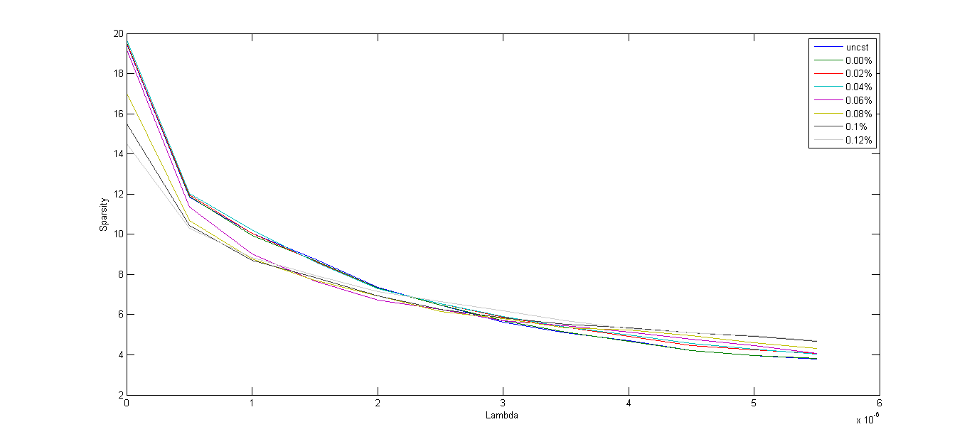
the composition is far from identical as many low-weighted stocks in the unregularized portfolios have large weights in the sparse portfolios. Moreover, Figure 1 shows the number of positive positions versus the regularization parameter $\lambda$ graph of the $\ell_{p}$ -norm regularized portfolios. With minor exception, increasing lambda almost always results in a more sparse solution which is consistent with our portfolio theory developed in Section 3.

Table 6: Results for

\ell_{p}

-norm Markowitz Regularized Portfolios with

\lambda=5.5e-6

: In-Sample Performance.

$\lambda$	5.5e-6
$m_{0}$	0.0002
$\phi$	0.00000
Mean	0.00025
Variance	4.12e-5
Sparsity	3
SO	0.55327
K	0.23209
GIS	0.21464

$\lambda$	5.5e-6
$m_{0}$	0.0004
$\phi$	0.00445
Mean	0.00025
Variance	4.12e-5
Sparsity	3
SO	0.55222
K	0.22999
GIS	0.21779

$\lambda$	5.5e-6
$m_{0}$	0.0006
$\phi$	0.01099
Mean	0.00046
Variance	4.05e-5
Sparsity	4
SO	0.38804
KMB	0.31953
K	0.16675
HSY	0.12568

$\lambda$	5.5e-6
$m_{0}$	0.0008
$\phi$	0.01886
Mean	0.00061
Variance	4.35e-5
Sparsity	4
KMB	0.35527
SO	0.27413
HSY	0.20689
AZO	0.16371

$\lambda$	5.5e-6
$m_{0}$	0.0010
$\phi$	0.02731
Mean	0.00098
Variance	5.76e-5
Sparsity	5
KMB	0.47565
HSY	0.2479
AZO	0.19227
REGN	0.06476
DUK	0.01942

$\lambda$	5.5e-6
$m_{0}$	0.0012
$\phi$	0.03645
Mean	0.00109
Variance	6.41e-5
Sparsity	6
KMB	0.43308
HSY	0.25649
AZO	0.18254
REGN	0.08895
DUK	0.02721
THC	0.01172

Refer to caption — Figure 1: Portfolio Sparsity

A comprehensive comparison of computational results between our $\ell_{p}$ -norm regularized model and the cardinality constrained portfolio selection (CCPS) model are reported in the Table 7. As can be seen in the table, our regularized $\ell_{p}$ -norm performs almost as well as theoretical possible—the difference of the variance estimation between the two models are within 0.2% in all cases and the difference of the mean estimation are within 0.02%. Therefore, compared to the computational intractable cardinality constrained portfolio optimization, our $\ell_{p}$ -norm regularized portfolio, which can be obtained in polynomial time, performs almost as well and seeks near optimal sparse portfolios.

Table 7: Comparison of Sparsity, Mean and Variance between the

\ell_{p}

-norm Model and CCPS (Daily Return).

	$\ell_{p}$ -norm				CCPS
	$\lambda$	Sparsity	Mean	Variance	Sparsity	Mean	Variance
$m_{0}=0.02\%\hskip 8.19447pt$	5.0e-7	9	0.05%	4.45%	9	0.05%	4.46%
	1.0e-6	7	0.03%	3.68%	7	0.04%	3.66%
	2.0e-6	5	0.03%	3.90%	5	0.04%	3.75%
	3.5e-6	4	0.02%	4.08%	4	0.04%	3.89%
	4.5e-6	3	0.02%	4.12%	3	0.04%	4.06%
$m_{0}=0.1\%\hskip 8.19447pt$	5.0e-7	10	0.06%	4.57%	10	0.05%	4.58%
	1.0e-6	7	0.10%	4.90%	7	0.10%	4.86%
	2.0e-6	7	0.09%	5.27%	5	0.09%	5.37%
	3.5e-6	6	0.09%	5.18%	6	0.09%	5.28%
	4.5e-6	6	0.09%	5.18%	6	0.09%	5.28%

4.2.2 Out-of-Sample Performance

[Brodie et al.(2009)] show that sparse portfolios are often more robust and thus outperform the portfolios with less sparsity in terms of out-of-sample performance. In their analysis, the no-shorting constraint ( $x\geq 0$ ) is taken as the most extreme sparsity inducing measure. We continued this investigation by taking the no-shorting constraint as the least extreme measure and adding the $\ell_{p}$ -norm regularizer onto the objective function. It is interesting to ask whether the sparsest portfolios will outperform other portfolio strategies with less sparsity.

Figure 2 and Figure 3 show the out-of-sample portfolio returns and variances obtained by the $\ell_{p}$ -norm regularized Markowitz model with $\lambda$ ranging from 5.0e-7 to 5.5e-6 and the CCPS, respectively. From Figure 2, we observe clearly that most of the plots go up slightly and then achieve its maximum, indicating that the portfolios with moderate sparsity (around 10) perform very well, even better than the Markowitz portfolio. However, with the continuously increasing of sparsity, the mean will go down dramatically and thus the regularized portfolios with extreme sparsity perform poorly in the sense of portfolio mean. Figure 3 shows that the variance of the regularized portfolios is increasing with a incremental rate with the increasing sparsity of the portfolios. However, though the highly sparse portfolios performs poorly in the sense of portfolio variance, the intermediate portfolios with about 10 companies suffered a 15-25% increase in variance which is also comparable to the CCPS integer portfolios.

Figure 4 shows the out-of-performance Sharpe ratios of our $\ell_{p}$ -norm regularized portfolio and the CCPS integer portfolio. Although the Markowitz portfolio (with $\lambda=0$ ) outperforms our $\ell_{p}$ -norm regularized model in terms of the out-of-sample Sharpe ratio, the sparse portfolios may be more implementable due to the transaction costs or logistical limitations reasons. Our results indicate that an intermediate sparse portfolio may get a comparable or at most only 10-20% cost in Sharpe ratio while reducing more construction costs. Also, the $\ell_{p}$ -norm regularized approach is competitive with the computationally gigantic integer approach in the sense of out-of-sample performance.

4.3 Shorting-Allowed Extension

Next we relaxed our constraint to allow the short-selling of stocks. We compare our model (2.6) with the $\ell_{1}$ -norm ball constrained portfolios studied by [DeMiguel et al.(2009b)], as the strategy may find sparse portfolios with improved out-of-sample Sharpe ratios.

4.3.1 $\ell_{p}$ -norm Regularized Model

Figure 5 shows that the shorting-allowed Markowitz portfolios behave eccentrically (also see Table 8), with the portfolio including all the stocks no matter the choice of the parameter $\phi$ . Meanwhile, our $\ell_{p}$ -norm regularized model (2.6) is able to reduce the number of investing stocks drastically. For example, only 22 stocks are involved in the Markowitz regularized portfolio for $\lambda=1e-6$ and $m_{0}=0.06\%$ , and thus there is a 95.2% reduction of the portfolio size. The parameter $\lambda$ can be regarded as a server to control the portfolio sparsity.

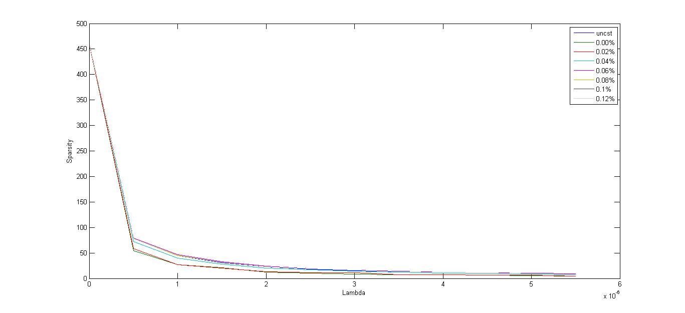
The out-of-sample results are similar to the shorting-prohibited case. From Table 8, we see that the Sharpe ratio tends to be the highest when $\lambda$ is not too large, and would decrease with the increasing of the parameter $\lambda$ . However, even for a significantly small $\lambda$ , the regularized portfolios are much more sparse (e.g. 79 versus 461), and of competitive or better performance while compared with the Markowitz portfolio. For larger values of $\lambda$ , there is a clear tradeoff between the portfolio sparsity and performance.

Table 8: Sharpe Ratio and Sparsity of shorting allowed

\ell_{p}

-norm regularized Model

$\lambda$	Spa	SRatio	Spa	SRatio	Spar	SRatio	Spar	SRatio
	$m_{0}=-\infty$		$m_{0}=0.02\%$		$m_{0}=0.06\%$		$m_{0}=0.1\%$
0	461.0	0.165	461.0	0.161	461.0	0.146	461.0	0.127
5.0e-7	78.1	0.156	58.7	0.161	79.3	0.161	78.2	0.166
1.0e-6	45.1	0.125	27.1	0.120	46.9	0.123	45.2	0.120
2.0e-6	22.9	0.159	13.4	0.159	24.4	0.159	23.4	0.155
2.5e-6	18.4	0.149	11.5	0.152	19.2	0.147	18.8	0.150
3.5e-6	13.4	0.120	7.6	0.120	14.3	0.118	13.4	0.121
4.5e-6	10.9	0.040	6.6	0.036	11.0	0.040	10.8	0.041
5.5e-6	8.5	0.024	4.9	0.023	8.9	0.024	8.6	0.027

Table 9: Sharpe Ratio and Sparsity of

\ell_{1}

-norm ball constrained Markowitz portfoliol

	$m_{0}=-\infty$		$m_{0}=0.02\%$		$m_{0}=0.06\%$		$m_{0}=0.1\%$
$\delta$	Spa	SRatio	Spa	SRatio	Spar	SRatio	Spar	SRatio
1.5	70.5	0.127	70.4	0.109	68.3	0.111	60.9	0.149
2	118.1	0.163	118.6	0.155	116.3	0.177	111.1	0.181

4.3.2 $\ell_{1}$ -norm Ball Constrained Model

For the purpose of comparison, we also post the results of $\ell_{1}$ -norm ball constrained portfolios on the same data set. The $\ell_{1}$ -norm ball constrained model considered in this section takes the following form

\begin{array}[]{rl}\min&\frac{1}{2}x^{T}Qx\\[5.69046pt] \mbox{s.t.}&e^{T}x=1,\\[5.69046pt] &m^{T}x\geq m_{0},\\[5.69046pt] &\|x\|_{1}\leq\delta,\\[5.69046pt] \end{array}

(4.1)

where $\delta\geq 1$ . Figure 6 shows the number of nonzero positions versus the threshold parameter $\delta$ of the $\ell_{1}$ -norm ball constrained portfolios. It is clear that the sparsity decreases at a fast speed with the increasing of $\delta$ . The left-most date points corresponds to the shorting-allowed Markowitz model where the $\ell_{1}$ -norm ball constraint is not effective while the right-most data points ( $\delta=1$ ) corresponds to the shorting-prohibited Markowitz mode where the $\ell_{1}$ -norm ball constraints takes its most effective role in inducing sparsity. However, even when $\delta=1$ , the average sparsity of the portfolio is around 15, which is much more dense than the shorting-allowed portfolio with $\lambda$ smaller than 3.5e-6.

We can make a detailed comparison between $\ell_{1}$ -norm ball constrained model and $\ell_{p}$ -norm regularization model by Table 8 and 9. It is easy to see that when $\delta$ equals 1.5 or 2, the out-of-sample performance of $\ell_{p}$ -norm models is similar to that of the $\ell_{1}$ -norm ball constrained portfolios but the former is much more sparse. However, the performance of the $\ell_{p}$ -norm models is surpassed when $\delta$ is increased. In that case, the $\ell_{1}$ -norm ball constrained portfolio achieves a better out-of-sample performance with the sacrifice of sparsity, see Figure 7. Moreover, the largest out-of-sample Sharpe Ratio is achieved when $\delta\approx 16$ . From this figure, we can also see that the shorting-allowed Markowitz Model (far left points) is better than shorting-prohibited Markowitz Model (far right points). This is consistent with the remark made by [Jagannathan and Ma(2003)] that when daily data is used, shorting-prohibited models perform almost as well.

4.4 $\ell_{1}$ -norm Ball Constrained $\ell_{p}$ -norm Regularized Model

In the last two sections, we have discussed the computational performance of the $\ell_{1}$ -norm ball constrained Markowitz model and the shorting-allowed $\ell_{p}$ -norm regularized Markowitz models (2.4) and (2.6) individually. Next, we consider the $\ell_{1}$ -norm ball constrained $\ell_{p}$ -norm regularized model (2.9) to investigate the relationship between the leverage (characterized by the $\ell_{1}$ -norm), the sparsity (induced mostly by the $\ell_{p}$ -norm) and the out-of-sample performance. According to the results of the $\ell_{1}$ -norm constrained model, we solve our regularized model combined with the $\ell_{1}$ -norm constraint with $\delta$ ranging from from 1.5 to 32 and $(\lambda,\phi)$ taking an array of values. This thorough approach are expected to give us a more structured picture of the relationship between the $\ell_{1}$ - and $\ell_{p}$ -norms as well as their relationship to the performance.

Table 10 reports the out-of-sample computational results for the cases where $\delta$ is taken as 1.5, 2 and 32, and $m_{0}$ is set as $-\infty$ and 0.04%. Since the $\ell_{1}$ -norm constrained $\ell_{p}$ -norm regularization enjoys the similar trend for different choices of $\delta$ , we don’t report the corresponding results for succinctness. From the table, we see clearly that the sparsity, in general, is antagonistic to performance. Thus, there exists a tradeoff between performance and sparsity. Though the performance varies for different values of $\lambda$ , a well performed portfolio can be obtained when $\lambda$ is smaller than 4.5e-06. And when $\lambda$ is not very large, say less then $2e-6$ , the sparsity need not come at a high price (of Sharpe ratio) and there are many sparse portfolios with comparable performance to the portfolios found with $\lambda=0$ . Also, we find that with the increase of $\lambda$ , the leverage of the resulting portfolio decreases significantly. Thus, it seems that the leverage of the portfolio is mostly determined by the choice of $\lambda$ . Moreover, we note that there appears to be little cross-effect between sparsity and leverage on performance.

Table 10: Sparsity and Sharpe Ratio of the Combined Model and

\ell_{1}

Norm model for S & P Data with Three Month Estimation Window: Out-of-Sample Performance

model/ $m_{0}$	$\lambda$	Spar	Leve	SRatio	Spar	Leve	SRatio	Spar	Leve	SRatio
		$\delta=1.5$			$\delta=2$			$\delta=32$
$\ell_{1}-\ell_{p}/-\infty$	5.0e-7	37.9	1.496	0.074	54.3	1.949	0.159	94.2	3.392	0.214
	2.0e-6	16.8	1.340	0.101	23.6	1.526	0.103	29.7	1.806	0.063
	4.5e-6	9.3	1.202	0.120	11.9	1.285	0.139	13.8	1.376	0.050
	8.0e-6	5.5	1.084	-0.094	6.8	1.130	-0.026	6.8	1.155	-0.138
	1.25e-5	4.1	1.049	-0.094	4.4	1.063	-0.132	4.4	1.068	-0.111
$\ell_{1}$ -norm/ $-\infty$	—	70.5	1.500	0.234	117.2	2.000	0.195	461	23.571	0.247
$\ell_{1}-\ell_{p}/0.04\%$	5.0e-7	35.1	1.496	0.074	56.6	1.948	0.177	94.4	3.414	0.226
	2.0e-6	16.3	1.338	0.114	23.6	1.523	0.115	29.8	1.808	0.086
	4.5e-6	9.6	1.197	0.105	12.0	1.284	0.138	13.6	1.378	0.053
	8.0e-6	5.6	1.088	-0.132	6.8	1.129	-0.006	6.7	1.143	-0.162
	1.25e-5	4.1	1.049	-0.098	4.4	1.063	-0.133	4.3	1.068	-0.115
$\ell_{1}$ -norm/ $0.04\%$	—	70.2	1.500	0.201	118.7	2.000	0.207	461.0	23.500	0.234

4.5 $\ell_{2}-\ell_{p}$ -norm Double Regularized Model

As mentioned in [DeMiguel et al.(2009)], the $\ell_{2}$ -norm constraint can be viewed as placing a prior on the 1/N strategy, thus it is reasonable to expect the results close to the 1/N strategy. Yet, most investors would not invest into a portfolio with huge number of stocks, which motivates us to develop a portfolio strategy with less stocks but similar to the 1/N strategy with competitive out-of-sample performance, especially for those passive investors. For this purpose, it is natural to consider the $\ell_{p}$ -norm regularization of the $\ell_{2}$ -norm constrained Markowitz model

\begin{array}[]{rl}\min&\frac{1}{2}x^{T}Qx+\lambda\|x\|_{p}^{p}\\[5.69046pt] \mbox{s.t.}&e^{T}x=1,\\[5.69046pt] &m^{T}x\geq m_{0},\\[5.69046pt] &\|x\|_{2}^{2}\leq\delta^{2},\\[5.69046pt] \end{array}

or its Lagranagin version (double regularization Markowitz model (2.10)) to see if we can obtain a portfolio that balances sparsity and uniform prior. The results of the $\ell_{2}-\ell_{p}$ model are shown in Table 11, with different choices of $\lambda$ and $\delta$ . The parameters $\mu$ and $\phi$ in the regularized model 2.10 are obtained from the dual variables of problem (4.5) with $\lambda=0$ . Seen from the result, the optimal portfolio obtained by the double regularization formulation would include all the stocks in the case that $\lambda=0$ for all values of $\delta$ , closely related to the 1/N strategy. Also, the portfolio becomes more sparse with the increasing of $\lambda$ and fixed $\delta$ , while more dense with the increasing of $\delta$ and fixed $\lambda$ . This trend shows a tradeoff between $\ell_{p}$ -norm regularization and $\ell_{2}$ -norm ball constraints.

It is also note that the strategy to invest all stocks doesn’t usually perform best in the sense of Sharpe ratio. For example, in the case that $\lambda$ =1.25e-5, $\delta$ =0.1 and $m_{0}$ =0.08%, we can find a portfolio with only 135 stocks yet with a high Sharpe ratio 0.575, which is much better than the Sharpe ratio 0.374 attained with $\lambda=0$ . Similar as the observation before, the extremely sparse portfolio often performs poorly showing a tradeoff between sparsity and performance.

Also, the most constricting delta ( $\delta=0.1$ ) had the highest performing portfolios, suggesting that the presence of a strong uniform prior on all stocks helps mitigate overfitting due to poor variance/covariance estimates. The out-of-sample performance was increasing in $\lambda$ when $\lambda$ was not too large. These moderately sparse, highly $\ell_{2}$ -norm constricted portfolios performed excellently (all had Sharpe Ratio near or above 0.5). Thus the $\ell_{2}$ and $\ell_{p}$ norms appear to exhibit synergy in reducing overfitting.

Table 12 lists the out-of-sample computational results of our $\ell_{2}-\ell_{p}$ double regularization model for international data with much more diversity. Compared with the results for S & P data, the overall performance is greatly enhanced, especially for the sparsest portfolios. Very surprisingly, we even find that a portfolio with two stocks perform quite well. And also we see that the cost of sparsity need not be high even for very sparse portfolios if the stock base is favorable.

Table 11: Sparsity and Sharpe Ratio of the

\ell_{2}-\ell_{p}

-Norm Double-Regularization Model for S& P Data with Three Month Estimation Window

		$\delta=0.1$		$\delta=0.2$		$\delta=0.3$		$\delta=0.4$
	$\lambda$	Spar	SRatio	Spar	SRatio	Spar	SRatio	Spar	SRatio
$m_{0}=0.00\%$	0	461.0	0.409	461.0	0.18	461.0	0.087	461.0	0.035
	5.0e-7	321.8	0.431	185.8	0.247	133.0	0.264	116.7	0.214
	2.0e-6	236.8	0.414	69.8	0.35	50.3	0.29	33.3	0.231
	4.5e-6	164.4	0.504	34.0	0.422	34.3	0.248	15.8	0.14
	8.0e-6	166.6	0.498	20.2	0.336	13.5	0.237	8.1	0.096
	1.25e-5	105.3	0.536	15.1	0.288	7.6	0.096	5.0	-0.083
$m_{0}=0.04\%$	0	461.0	0.389	461.0	0.181	461.0	0.085	461.0	0.046
	5.0e-7	321.8	0.405	181.3	0.25	127.0	0.236	111.8	0.233
	2.0e-6	233.3	0.385	63.8	0.374	46.2	0.27	36.9	0.251
	4.5e-6	189.6	0.414	34.8	0.43	26.5	0.258	22.3	0.147
	8.0e-6	188.9	0.52	20.9	0.376	11.3	0.201	8.2	0.122
	1.25e-5	132.5	0.553	15.3	0.31	7.8	0.087	4.9	-0.082
$m_{0}=0.08\%$	0	460.9	0.374	461.0	0.183	461.0	0.089	461.0	0.052
	5.0e-7	343.7	0.376	198.3	0.286	144.7	0.246	120.6	0.243
	2.0e-6	254.9	0.366	73.0	0.39	63.4	0.212	32.6	0.222
	4.5e-6	179.6	0.379	35.4	0.421	25.6	0.288	27.0	0.212
	8.0e-6	165.3	0.444	34.5	0.295	14.2	0.194	8.2	0.114
	1.25e-5	134.6	0.575	16.1	0.265	7.8	0.097	5.1	-0.079

Table 12: Sparsity and Sharpe Ratio of the

\ell_{2}-\ell_{p}

-Norm Double-Regularization Model for International Data with Three Month Estimation Window

		$\delta=0.1$		$\delta=0.2$		$\delta=0.3$		$\delta=0.4$
	$\lambda$	Spar	SRatio	Spar	SRatio	Spar	SRatio	Spar	SRatio
$m_{0}=0.00\%$	0	749.8	0.569	750.0	0.528	749.8	0.509	749.9	0.497
	5.0e-7	265.0	0.611	84.8	0.477	60.8	0.443	31.6	0.439
	2.0e-6	109.0	0.58	23.4	0.452	14.9	0.439	8.1	0.419
	4.5e-6	65.7	0.578	12.3	0.461	5.1	0.417	3.8	0.435
	8.0e-6	60.4	0.602	7.67	0.462	3.4	0.415	2.4	0.433
	1.25e-5	32.2	0.62	5.4	0.407	2.6	0.424	2.25	0.433
$m_{0}=0.04\%$	0	749.9	0.615	749.9	0.554	750.0	0.524	750.0	0.508
	5.0e-7	270.8	0.619	83.8	0.485	48.7	0.445	32.4	0.437
	2.0e-6	115.0	0.606	24.5	0.459	12.0	0.441	8.2	0.418
	4.5e-6	67.3	0.599	12.58	0.46	5.3	0.416	3.8	0.429
	8.0e-6	46.5	0.621	8.0	0.456	3.4	0.413	2.4	0.434
	1.25e-5	33.5	0.628	5.5	0.404	2.6	0.423	2.3	0.433
$m_{0}=0.08\%$	0	749.7	0.637	750.0	0.588	749.8	0.544	749.9	0.524
	5.0e-7	291.8	0.649	88.2	0.486	49.3	0.446	38.0	0.439
	2.0e-6	128.6	0.692	26.3	0.467	12.3	0.434	8.3	0.417
	4.5e-6	87.3	0.631	13.1	0.455	5.3	0.414	4.17	0.429
	8.0e-6	52.8	0.623	8.5	0.461	3.5	0.41	2.42	0.434
	1.25e-5	38.8	0.625	5.8	0.4	2.6	0.4	2.3	0.433

5 Discussions and Conclusions

5.1 $\ell_{p}$ -norm regularized Dynamic Portfolios

A closely related application to our model is the dynamic portfolio selection. Instead of seeking a sparse portfolio, we are looking for a sparse adjustment to an already existing portfolio. Consider the following cardinality constrained optimization model.

\begin{array}[]{rl}\min&\frac{1}{2}x^{T}Qx-c^{T}x\\[5.69046pt] \mbox{s.t.}&e^{T}x=1\\[2.84544pt] &x\geq 0\\[2.84544pt] &\|x-a\|_{0}\leq K,\end{array}

(5.1)

Here the $a$ -vector is a feasible portfolio ( $e^{T}a=1$ and $a\geq 0$ ), representing the current state of our dynamic portfolio. Similar to the Markowitz model, the dynamic portfolio has found many applications. One is the situation where implementing the portfolio takes a significant amount of time (perhaps we must execute our orders sequentially with long delays in-between) and we wish our first orders to constitute an near-optimal portfolio. Another is the situation where our estimates $Q$ and $c=\phi m$ are themselves varying over time, enough to warrant a re-balancing, yet we still have limits on trading—either due to transaction costs or structural limitations.

This model has a non-differentiable point in the middle of the feasible region ( $x=a$ ), but can be reformulated (by substitution: $y=x-a$ ) to achieve a model very similar to the non-dynamic sparse portfolio model:

\begin{array}[]{rl}\min&\frac{1}{2}y^{T}Qy+Qa^{T}y-c^{T}y\\ \mbox{s.t.}&e^{T}y=0\\ &y\geq-a\\ &\|y\|_{0}\leq K,\end{array}

(5.2)

We note that the objective function is still a quadratic function, and that the constraints are also of the same shape. Instead of solving the original model (5.2), we consider the following $p$ norm regularized dynamic Markowitz model

\begin{array}[]{rl}\min&\frac{1}{2}y^{T}Qy+(a^{T}Q-c^{T})y+\lambda\|y\|_{p}^{p}\\[8.5359pt] \mbox{s.t.}&e^{T}y=0,\\[5.69046pt] &y\geq-a.\end{array}

(5.3)

By letting $y=y^{+}-y^{-}$ and using the concavity of $\|\cdot\|_{p}^{p}$ , we know the regularized model (5.3) can be equivalently written as

\begin{array}[]{rl}\min&\frac{1}{2}(y^{+}-y^{-})^{T}Q(y^{+}-y^{-})+(a^{T}Q-c^{T})(y^{+}-y^{-})+\lambda\|y^{+}\|_{p}^{p}+\lambda\|y^{-}\|_{p}^{p}\\[5.69046pt] \mbox{s.t.}&e^{T}y^{+}-e^{T}y^{-}=0,\\[2.84544pt] &y^{+}-y^{-}\geq-a,\\[2.84544pt] &y^{+}\geq 0,\,y^{-}\geq 0,\end{array}

(5.4)

which can be further simplified to the following model

\begin{array}[]{rl}\min&\frac{1}{2}(y^{+}-y^{-})^{T}Q(y^{+}-y^{-})+(a^{T}Q-c^{T})(y^{+}-y^{-})+\lambda\|y^{+}\|_{p}^{p}+\lambda\|y^{-}\|_{p}^{p}\\[5.69046pt] \mbox{s.t.}&e^{T}y^{+}-e^{T}y^{-}=0,\\[2.84544pt] &y^{+}\geq 0,\,\,\,0\leq y^{-}\leq a,\end{array}

(5.5)

Similar as the non-dynamic $\ell_{p}$ - norm portfolio model, this resulting $\ell_{p}$ -norm model can also be solved by the second order interior interior point method.

5.2 Conclusions

In this paper, we propose an $\ell_{p}$ -norm regularized model with/without shortsale constraints to seek near-optimal sparse portfolios to reduce the complexity of portfolio implementation and management. We also study the impact of the $\ell_{1}$ and $\ell_{2}$ norms and their cross-effects on overfitting. Theoretical results is established to guarantee the sparsity of the novel portfolio strategy. Computational evidence also clearly shows that the $\ell_{p}$ -norm regularized portfolio is able to choose sparsity with completely flexibility while still maintaining satisfactory out-of-sample performance—comparable to that of the NP cardinality-constrained portfolios.

We find that the $\ell_{1}$ -norm can be viewed as a prior on the optimal level of portfolio leverage; a small $\ell_{1}$ -penalty can improve performance. The $\ell_{1}$ norm greatly reduces the feasible region helping algorithms converge quickly. It also is shown to be synonymous with leverage—a very important financial term and quantity of great theoretical interest.

Meanwhile the $\ell_{2}$ -norm can be viewed as a prior on the estimated covariances; we find that a large $\ell_{2}$ -penalty can greatly improve performance, It also could improve tractability by bounding the feasible region. And $\ell_{2}$ -norm and the $\ell_{p}$ -norm have positive cross-effects on performance—the combined model consistently portfolios outperformed all others.

Generally, when we do not pursue the most sparse portfolio,then the cost of sparsity is low—especially when the original portfolio of stocks is diverse. And our research provides a toolset to evaluate the tradeoffs between sparsity and out-of-sample performance.

Our models also importantly provide a theoretical framework. In this framework, sparsity can be studied in relation to leverage, correlation, Sharpe-Ratio and financial theory, where both practical bounds and qualitative insights can be made.

6 Appendix

6.1 Appendix I: Proofs of the Propositions

Proof of Theorem 3.1. Since the second-order necessary condition of (2.4) holds at the point $\bar{x}$ , the sub-Hessian matrix of the objective function corresponding to the indices $\bar{P}$

\bar{Q}-\frac{\lambda}{4}\bar{X}^{-3/2}\succeq 0

on the null space of $e$ . This means the projected Hessian matrix

\left(I-\frac{1}{K}ee^{T}\right)\left(\bar{Q}-\frac{\lambda}{4}\bar{X}^{-3/2}\right)\left(I-\frac{1}{K}ee^{T}\right)

is positive semidefinite. By direct calculation, we know that the $i$ th diagonal entry of the projected Hessian matrix is given by

L_{i}-\frac{\lambda}{4}\left((\bar{x}_{i})^{-3/2}\left(1-\frac{2}{K}\right)+\frac{\sum_{j\in\bar{P}}(\bar{x}_{j})^{-3/2}}{K^{2}}\right)\geq 0,

(6.1)

and also the trace of projected Hessian matrix

\sum_{i\in\bar{P}}L_{i}-\frac{\lambda}{4}\frac{K-1}{K}\sum_{i\in\bar{P}}(\bar{x}_{i})^{-3/2}\geq 0.

The quantity $\sum_{i\in\bar{P}}(\bar{x}_{i})^{-3/2}$ , with $\sum_{i\in\bar{P}}\bar{x}_{i}=1$ , achieves its minimum at $\bar{x}_{i}=1/K$ for all $i\in\bar{P}$ with the minimum value $K\cdot K^{3/2}$ . Thus,

\frac{\lambda}{4}(K-1)K^{3/2}\leq\sum_{i\in\bar{P}}L_{i},

(K-1)K^{3/2}\leq\frac{4\sum_{i\in\bar{P}}L_{i}}{\lambda},

which complete the proof of the first claim. Moreover, from (6.1) we have

\frac{\lambda}{4}\left((\bar{x}_{i})^{-3/2}\left(1-\frac{2}{K}\right)+\frac{\sum_{j\in\bar{P}}(\bar{x}_{j})^{-3/2}}{K^{2}}\right)\leq L_{i}.

\frac{\lambda}{4}\left((\bar{x}_{i})^{-3/2}\left(1-\frac{1}{K}\right)^{2}+\frac{\sum_{j\in\bar{P},j\neq i}(\bar{x}_{j})^{-3/2}}{K^{2}}\right)\leq L_{i},

which implies

\frac{\lambda}{4}(\bar{x}_{i})^{-3/2}\left(1-\frac{1}{K}\right)^{2}\leq L_{i}.

(6.2)

Hence, if $L_{i}=0$ , we must have $K=1$ so that $\bar{x}_{i}$ is the only non-zero entry in $\bar{x}$ and $\bar{x}_{i}=1$ . Otherwise, from (6.2), we have the desired second statement in the theorem.

Proof of Theorem 3.2.） (i) Assume the contrary that $\bar{P}^{+}\cap\bar{P}^{-}\neq\emptyset$ . Then there exists an index $j$ such that $\bar{x}_{j}^{+}>0$ and $\bar{x}_{j}^{-}>0$ . Let $\lambda_{1}$ and $\lambda_{2}\,(\leq 0)$ be the optimal Lagrangian multiplier associated with the constraints of (2.9). Since $(x^{+},x^{-})$ is a KKT point of (2.9), it holds that

\left\{\begin{array}[]{c}\displaystyle\left[Q(\bar{x}^{+}-\bar{x}^{-})\right]_{i}-c_{i}+{\lambda\over 2\sqrt{(\bar{x}^{+})_{i}}}-\lambda_{1}-\lambda_{2}=0\\ \displaystyle\left[Q(\bar{x}^{-}-\bar{x}^{+})\right]_{i}+c_{i}+{\lambda\over 2\sqrt{(\bar{x}^{-})_{i}}}+\lambda_{1}-\lambda_{2}=0\end{array}\right..

(6.3)

By adding the two equalities above, we have

{\lambda\over 2\sqrt{(\bar{x}^{+})_{i}}}+{\lambda\over 2\sqrt{(\bar{x}^{-})_{i}}}-2\lambda_{2}=0.

(6.4)

However, since $(\bar{x}^{+})_{i}>0,\,\,(\bar{x}^{-})_{i}>0$ and $\lambda_{2}\leq 0$ , the equality (6.4) cannot hold. This contradiction shows that $\bar{P}^{+}\cap\bar{P}^{-}\neq\emptyset$ . (ii,iii) Since the proof of the remainder parts of this theorem is similar to that of Theorem 1, we omit the details.

Proof of Theorem 3.3 .） The proof of this theorem is similar to that of Theorem 1. We omit the details.

6.2 Appendix II: Polynomial Time Interior Point Algorithms

Most nonlinear optimization solvers can only guarantee to compute a first-order KKT solution. In this section, we extend the interior-point algorithm described in [Bian et al.(2012)] to solve the following generally $\ell_{p}$ -norm regularized model

\begin{array}[]{rl}\min&\displaystyle f(x):=\frac{1}{2}\,\,x^{T}Qx-c^{T}x+\lambda\|x\|^{p}_{p}\\[8.5359pt] \mbox{s.t.}&Ax=b,\\[2.84544pt] &x\geq 0,\end{array}

(6.5)

where $A$ is a matrix in $\Re^{p\times n}$ , $b$ is a vector in $\Re^{p}$ and the feasible region is strictly feasible. For simplicity, we fix $p={1\over 2}$ .

Naturally, we would start from an interior-point feasible solution such as the analytical of the feasible set, and let the iterative algorithm to decide which entry goes to zero. This is the basic idea of affine scaling algorithm developed in [Bian et al.(2012)] for regularized nonconvex programming. The algorithm starts from an initial interior-point solution, then follows an interior feasible path and finally converges to either a global minimizer or a second-order KKT solution. At each step, it chooses a new interior point which produces a reduction to the objective function by an affine-scaling trust-region iteration.

Specifically, give an interior point $x^{k}$ of the feasible region, the algorithm looks for an objective reduction by a update from $x^{k}$ to $x^{k+1}$ . Let $d^{k}$ be a vector in $\Re^{p}$ satisfying $Ad^{k}=0$ and $x^{k+1}:=x^{k}+d^{k}>0$ . Using the second Taylor expansion of $f(\cdot)$ , we know

f(x^{k+1})\approx f(x^{k})+\frac{1}{2}(d^{k})^{T}\big(Q-\frac{\lambda}{4}(X^{k})^{-3/2}\big)d^{k}+\big(Qx^{k}-c+\frac{\lambda}{2\sqrt{x^{k}}}\big)^{T}d^{k},

where $X^{k}={\rm Diag}(x^{k})$ . For given $\varepsilon\in(0,1]$ , we solve the ellipsoidal trust-region constrained problem

\begin{array}[]{rl}\min&\displaystyle\frac{1}{2}(d^{k})^{T}\big(Q-\frac{\lambda}{4}(X^{k})^{-3/2}\big)d^{k}+\big(Qx^{k}-c+\frac{\lambda}{2\sqrt{x^{k}}}\big)^{T}d^{k}\\[8.5359pt] \mbox{s.t.}&Ad^{k}=0,\\[5.69046pt] &\|X_{k}^{-1}d^{k}\|^{2}\leq\beta^{2}\varepsilon<1,\end{array}

to obtain the direction $d^{k}$ . By letting $\tilde{d^{k}}=X_{k}^{-1}d^{k}$ , we can recast the above ellipsoidal trust-region constrained problem above as a ball-constrained quadratic problem

\begin{array}[]{rl}\min&\displaystyle\frac{1}{2}(\tilde{d}^{k})^{T}X^{k}\big(Q-\frac{\lambda}{4}(X^{k})^{-3/2}\big)X^{k}\tilde{d}^{k}+\big(Qx^{k}-c+\frac{\lambda}{2\sqrt{x_{k}}}\big)^{T}X^{k}\tilde{d}^{k},\\[8.5359pt] \mbox{s.t.}&AX_{k}\tilde{d}^{k}=0,\\[2.84544pt] &\|\tilde{d}^{k}\|^{2}\leq\beta^{2}\varepsilon.\end{array}

(6.6)

Note that problem (6.6) can be solved efficiently even when it is nonconvex (see [Bian et al.(2012)]).

Let $\widetilde{Q}^{k}=X_{k}QX_{k}-\frac{\lambda}{4}\sqrt{X^{k}}$ and $\tilde{c}^{k}=X_{k}(Qx^{k}-c)+\frac{\lambda}{2}\sqrt{x^{k}}$ . If $\widetilde{Q}_{k}$ is semidefinite, the solution $\tilde{d}^{k}$ of problem (6.6) satisfies the following necessary and sufficient conditions:

\left\{\begin{array}[]{l}(\widetilde{Q}^{k}+\mu_{k}I)\tilde{d}^{k}-(AX^{k})^{T}y_{k}=-\tilde{c}^{k},\\[2.84544pt] AX^{k}\tilde{d}^{k}=0,\\[2.84544pt] \mu_{k}\geq 0,\,\|\tilde{d}^{k}\|^{2}\leq\beta^{2}\varepsilon,\,\mu_{k}(\|\tilde{d}^{k}\|^{2}-\beta^{2}\varepsilon)=0.\end{array}\right.

(6.7)

In the case that $\widetilde{Q}^{k}$ is indefinite, it holds that

\left\{\begin{array}[]{l}(\widetilde{Q}^{k}+\mu_{k}I)\tilde{d}^{k}-(AX^{k})^{T}y_{k}=-\tilde{c}^{k},\\[2.84544pt] AX_{k}\tilde{d}^{k}=0,\\[2.84544pt] \mu_{k}\geq 0,\,N_{k}^{T}\widetilde{Q}^{k}N_{k}+\mu_{k}I\succeq 0,\\[2.84544pt] \|\tilde{d}^{k}\|=\beta\sqrt{\varepsilon},\end{array}\right.

(6.8)

where $N_{k}$ is an orthogonal basis spanning the space of $X^{k}A^{T}$ .

To evaluate the performance of the affine scaling method, we need the definitions of $\varepsilon$ scaled first-order and second-order KKT solutions. $x^{*}$ is said to be an $\epsilon$ scaled first-order KKT solution of (6.5) if there exists a $y^{*}\in\Re^{p}$ such that

\left\{\begin{array}[]{l}\displaystyle\|X^{*}(Qx^{*}-c)+\frac{\lambda}{2}\sqrt{x^{*}}-X^{*}A^{T}y^{*}\|\leq\epsilon,\\[2.84544pt] Ax^{*}=b,\\[2.84544pt] x^{*}\geq 0.\end{array}\right.

(6.9)

Furthermore, if $\displaystyle X^{*}QX^{*}-\frac{\lambda}{4}\sqrt{X^{*}}+\sqrt{\epsilon}I$ is also semidefinite on the null space of $X^{*}A^{T}$ , we call $x^{*}$ an $\epsilon$ scaled second-order KKT solution. If $\varepsilon=0$ , the $\varepsilon$ scaled first-order KKT solution reduces to

X^{*}(Qx^{*}-c)+\frac{\lambda}{2}\sqrt{x^{*}}-X^{*}A^{T}y^{*}=0,

which is exactly the first-order condition of (6.5). In this case, the $\varepsilon$ scaled second-order condition collapses to

N^{T}X^{*}QX^{*}N-\frac{\lambda}{4}N^{T}\sqrt{X^{*}}N\succeq 0

(6.10)

where $N$ is an orthogonal basis spanning the space of $X^{*}A^{T}$ . By direct computation, we know (6.10) recovers exactly the second-order optimality condition of problem (6.5).

For the convergence analysis of our proposed interior-point algorithm, we make the following standard assumption. For any given $x^{0}\geq 0$ such that $Ax=b$ , there exists $R\geq 1$ such that

\sup\{\|x\|_{\infty}:f(x)\leq f(x_{0}),Ax=b,x\geq 0\}\leq R.

Under the assumption above, we are able to establish the next theorem showing that the affine scaling is able to obtain either an $\varepsilon$ -scaled second-order KKT solution or an $\varepsilon$ global minimizer in polynomial time.

Theorem 6.4

Let $\varepsilon\in(0,1]$ . There exists a positive number $\tau$ such that the proposed second-order interior point obtains either an $\varepsilon$ scaled second-order KKT solution or $\varepsilon$ global minimizer of (6.5) in no more than $O(\varepsilon^{-3/2})$ iterations provided that $\beta\in(0,\,\tau)$ .

Proof: With loss of generality, we assume the radius $R=1$ in the assumption. To proceed the proof of this theorem, we first introduce the following Lemma.

Lemma 6.1

If $\mu_{k}>\lambda/6\|\tilde{d}^{k}\|$ holds for all $k=0,1,2,\ldots$ , then the second-order interior point algorithm produces an $\varepsilon$ global minimizer of (6.5) in at most $O(\varepsilon^{-3/2})$ iterations.

Proof: By the Taylor expansion of $\sqrt{\cdot}$ , it is easily to show that

f(x^{k+1})-f(x^{k})\leq\frac{1}{2}\big\langle\tilde{d}^{k},\,\widetilde{Q}^{k}\tilde{d}^{k}\big\rangle+\big\langle\tilde{c}^{k},\,\tilde{d}^{k}\rangle+\frac{3\lambda}{48}\|\tilde{d}_{k}\|^{3}.

From (6.7) and (6.8), then

\begin{array}[]{rl}f(x^{k+1})-f(x^{k})&\displaystyle\leq\frac{1}{2}\big\langle\tilde{d}^{k},\,\widetilde{Q}^{k}\tilde{d}^{k}\big\rangle+\big\langle-\widetilde{Q}^{k}\tilde{d}^{k}-\mu_{k}\tilde{d}^{k}+(AX_{k})^{T}y_{k},\,\tilde{d}^{k}\rangle+\frac{3\lambda}{48}\|\tilde{d}^{k}\|^{3}\\[5.69046pt] &\displaystyle=-\frac{1}{2}\tilde{d}^{k}\widetilde{Q}^{k}\tilde{d}^{k}-\mu_{k}\|\tilde{d}^{k}\|^{2}+\frac{3\lambda}{48}\|\tilde{d}^{k}\|^{3}\\[5.69046pt] &\displaystyle=-\frac{1}{2}(v^{k})^{T}(N_{k})^{T}\widetilde{Q}^{k}N_{k}v^{k}-\mu_{k}\|\tilde{d}^{k}\|^{2}+\frac{3\lambda}{48}\|\tilde{d}^{k}\|^{3}\\[5.69046pt] &\displaystyle\leq\frac{\mu_{k}}{2}\|v^{k}\|^{2}-\mu_{k}\|\tilde{d}^{k}\|^{2}+\frac{\lambda}{48}\|\tilde{d}^{k}\|^{3}\\[5.69046pt] &\displaystyle=-\frac{\mu_{k}}{2}\|\tilde{d}^{k}\|^{2}+\frac{3\lambda}{48}\|\tilde{d}^{k}\|^{3}\\[5.69046pt] &\displaystyle\leq-\frac{1}{8}\mu_{k}\|\tilde{d}_{k}\|^{2},\end{array}

(6.11)

where the second inequality follows from the semidefiniteness of $(N_{k})^{T}(\widetilde{Q}^{k})N_{k}+\mu_{k}I$ and the last inequality comes from the relationship that $\|\tilde{d}_{k}\|<6\mu_{k}/\lambda$ . Combining (6.11) with the fact that $\|\tilde{d}^{k}\|=\beta\sqrt{\varepsilon}$ due to $\mu_{k}>0$ , we further have

f(x^{k})-f(x^{0})\leq-\frac{1}{8}\sum_{j=0}^{k-1}\mu_{j}\|\tilde{d}_{j}\|^{2}\leq-\frac{\lambda}{48}k\big({\beta^{2}\varepsilon}\big)^{3/2}

and hence the interior-point algorithm produces an $\varepsilon$ global minimizer in $O(\varepsilon^{-\frac{3}{2}})$ iterations.

In what follows, we pay more attentions to the case where $\mu_{k}\leq\lambda/6\|\tilde{d}^{k}\|$ for some $k$ .

Lemma 6.2

Let $\beta\leq\min\{\frac{1}{2},\sqrt{2\over\lambda},\frac{3}{(18\sqrt{2}+2)\lambda}\}$ . If there exists some $k$ such that $\mu_{k}\leq\frac{\lambda}{6}\|\tilde{d}^{k}\|$ , then $x^{k+1}$ is an $\varepsilon$ second-order KKT solution of (6.5).

Proof: (i) We firstly show $x^{k+1}$ is an $\varepsilon$ scaled first order KKT solution when $\beta$ is restricted into the special range. From (6.7) and (6.8), it follows that

-\mu_{k}\tilde{d}^{k}=X^{k}({Q}x^{k+1}-c)-\frac{\lambda}{4}\sqrt{X^{k}}\tilde{d}^{k}+\frac{\lambda\sqrt{x^{k}}}{2}-X^{k}A^{T}y^{k},

which implies that

Qx^{k+1}-c-A^{T}y^{k}=\frac{\lambda}{4}(X^{k})^{-1/2}\tilde{d}^{k}-\frac{\lambda}{2}(x^{k})^{-1/2}-\mu_{k}(X^{k})^{-1}\tilde{d}^{k}.

Therefore, we have

\begin{array}[]{rl}&\displaystyle\|X^{k+1}(Qx^{k+1}-c)+\frac{\lambda\sqrt{x^{k+1}}}{2}-X^{k+1}A^{T}y^{k}\|\\[2.84544pt] =&\displaystyle\|\frac{\lambda\sqrt{x^{k+1}}}{2}-\frac{\lambda}{2}X^{k+1}(x^{k})^{(-1/2)}+\frac{\lambda}{4}X^{k+1}({X^{k}})^{-1/2}\tilde{d}^{k}-\mu_{k}X^{k+1}(X^{k})^{-1}\tilde{d}^{k}\|\\[7.11317pt] \leq&\displaystyle\|\frac{\lambda\sqrt{x^{k+1}}}{2}-\frac{\lambda}{2}X^{k+1}(x^{k})^{(-1/2)}+\frac{\lambda}{4}X^{k+1}({X^{k}})^{-1/2}\tilde{d}^{k}\|+\mu_{k}\|X^{k+1}(X^{k})^{-1}\tilde{d}^{k}\|\\[7.11317pt] \leq&\displaystyle\frac{\lambda}{2}\|\sqrt{X^{k}}\|_{\infty}\|\sqrt{\tilde{d}^{k}+e}-e-\frac{1}{2}\tilde{d}^{k}+\frac{1}{2}(\tilde{d}^{k})^{2}\|+\mu_{k}\|\tilde{d}^{k}\|(1+\|\tilde{d}^{k}\|)\end{array}

(6.12)

Since the condition $\mu_{j}>{\lambda\over 6}\|\tilde{d}^{j}\|$ holds for $j=0,1,2\ldots,k-1$ , by the proof of Lemma 1, we have $f(x^{k})\leq f(x^{0})$ , which together with Assumption 1 implies $\|x^{k}\|_{\infty}\leq 1$ . Moreover, we know from the proof of Lemma 4 in [Bian et al.(2012)] that

\|\sqrt{\tilde{d}^{k}+e}-e-\frac{1}{2}\tilde{d}^{k}+\frac{1}{2}({\tilde{d}}^{k})^{2}\|\leq\frac{1}{2}\|\tilde{d}^{k}\|^{2}

and hence

\begin{array}[]{rl}&\displaystyle\|(X^{k+1})(Qx^{k+1}-c)+\frac{\lambda\sqrt{x^{k+1}}}{2}-X^{k+1}A^{T}y^{k}\|\\[8.5359pt] \leq&\displaystyle\frac{\lambda}{4}\|\tilde{d}^{k}\|^{2}+\frac{3}{2}\mu_{k}\|\tilde{d}^{k}\|\leq\frac{\lambda}{2}\|\tilde{d}^{k}\|^{2}\leq\varepsilon,\end{array}

which means $x^{k+1}$ is an $\varepsilon$ scaled first-order KKT solution.

(ii) Again from (6.7) and (6.8), we know that

X^{k}QX^{k}-\frac{\lambda}{4}\sqrt{X^{k}}+\mu_{k}I

is positive semidefinite on the null space that $X^{k}A^{T}$ . Let $N_{k}$ be the orthogonal basis of this null space and it therefore holds

N_{k}^{T}(X^{k}QX^{k}-\frac{\lambda}{4}\sqrt{X^{k}})N_{k}\succeq-\mu_{k}I\succeq-\frac{\lambda}{6}\beta\sqrt{\varepsilon}I.

(6.13)

Clearly, $N_{k+1}:=(X^{k+1})^{-1}X^{k}N_{k}$ is a basis of the null space of $X^{k+1}A^{T}$ . By simple algebraic computation, we can easily obtain that

\begin{array}[]{rl}&\displaystyle N_{k+1}^{T}\left[X^{k+1}QX^{k+1}-\frac{\lambda}{4}\sqrt{X^{k+1}}+\sqrt{\varepsilon}I\right]N_{k+1}\\[11.38092pt] =&\displaystyle N_{k}^{T}(X^{k}QX^{k}-{\lambda\over 4}\sqrt{X^{k}})N_{k}+\sqrt{\varepsilon}N_{k}^{T}\left[X_{k+1}^{-2}(X^{k})^{2}\right]N_{k}\\[5.69046pt] &\displaystyle+{\lambda\over 4}N_{k}^{T}\sqrt{X^{k}}\big[I-(X^{k})^{3/2}(X^{k+1})^{-3/2}\big]N_{k}\\[11.38092pt] \displaystyle\succeq&-\frac{\lambda}{6}\beta\sqrt{\varepsilon}I+\sqrt{\varepsilon}N_{k}^{T}(I+D_{k})^{-2}N_{K}+{\lambda\over 4}N_{k}^{T}\sqrt{X^{k}}\big[I-(I+D_{k})^{-3/2}\big]N_{k}\end{array}

(6.14)

where $D_{k}={\rm Diag}(\tilde{d}^{k})$ . Since $\|\tilde{d}^{k}\|\leq\beta\sqrt{\varepsilon}\leq{1\over 2}<1$ , we know

(I+D_{k})^{-2}\succeq(1+\beta\sqrt{\varepsilon})^{-2}I\,\succeq{1\over 4}I

(6.15)

and

I-(I+D_{k})^{-3/2}\succeq\big[1-(1-\beta\sqrt{\varepsilon})^{-3/2}\big]I.

(6.16)

Moreover, the mean-value theorem applied to the function $x^{-3/2}$ yields that

1-(1-\beta\sqrt{\varepsilon})^{-3/2}=-{3\over 2}\beta\sqrt{\varepsilon}\theta^{-5/2},

where $\theta$ is in the open interval $(1-\beta\sqrt{\varepsilon},\,1)$ . Note that $\beta\sqrt{\varepsilon}\leq{1\over 2}$ , then it holds that

1-(1-\beta\sqrt{\varepsilon})^{-3/2}\geq-6\sqrt{2}\beta\sqrt{\varepsilon}.

(6.17)

By substituting (6.15), (6.16) and (6.17) into (6.14), we immediately get that

N_{k+1}^{T}\left[X^{k+1}QX^{k+1}-\frac{\lambda}{4}\sqrt{X^{k+1}}+\sqrt{\varepsilon}I\right]N_{k+1}\succeq({1\over 4}-{3\sqrt{2}\beta\lambda\over 2}-{\lambda\over 6}\beta)\sqrt{\varepsilon}I\succeq 0.

Thus $x^{k+1}$ is an $\varepsilon$ scaled second-order KKT solution.

According to the above two lemmas, we know the proposed second order interior point obtains either an $\varepsilon$ scaled second KKT solution or $\varepsilon$ global minimizer in no more than $O(\varepsilon^{-3/2})$ iterations provided that $\beta_{k}\leq\min\{\frac{1}{2},\sqrt{2\over\lambda},\frac{3}{(18\sqrt{2}+2)\lambda}\}$ . This completes the proof of this Theorem.

References

[Bertsimas and Shioda(2009)] Bertsimas, D., R. Shioda. 2009. Algorithm for cardinality-constrained quadratic optimization. Comput. Optim. Appl. 43(1) 1–22.
[Bian et al.(2012)] Bian, W., X. J. Chen, Y. Y Ye. 2012. Complexity analysis of interior point algorithms for non-lipschitz and nonconvex minimization. Preprint .
[Bienstock(1996)] Bienstock, D. 1996. Computational study of a family of mixed-integer quadratic programming problems. Math. Programming 74(2) 121–140.
[Boyle et al.(2012)] Boyle, P., L. Garlappi, R. Uppal, T. Wang. 2012. Keynes meets markowitz: The trade-off between familiarity and diversification. Management Sci. 58(2) 253–272.
[Brodie et al.(2009)] Brodie, J., I. Daubechies, C. De Mol, D. Giannone, I. Loris. 2009. Sparse and stable markowitz portfolios. Proc. Natl. Acad. Sci. 106(30) 12267–12272.
[Cesarone et al.(2009)] Cesarone, F., A. Scozzari, F. Tardella. 2009. Efficient algorithms for mean-variance portfolio optimization with hard real-world constraints. Giornale dell’Istituto Italiano degli Attuari 72 37–56.
[Chang et al.(2000)] Chang, T. J., N. Meade, J. E. Beasley, Y. M. Sharaiha. 2000. Heuristics for cardinality constrained portfolio optimisation. Computers & Operations Research 27(13) 1271–1302.
[Chartrand(2007)] Chartrand, R. 2007. Exact reconstruction of sparse signals via nonconvex minimization. IEEE Singal Proc. Let. 14(10) 707–710.
[Chen et al(2010)] Chen, X. J., F. M. Xu, Y. Y. Ye. 2010. Lower Bound Theory of Nonzero Entries in Solutions of $\ell_{2}-\ell_{p}$ Minimization. SIAM J. Sci. Comput. 32(5) 2832–2852.
[DeMiguel et al.(2009)] DeMiguel, V., L. Garlappi, F. J. Nogales, R. Uppal. 2009a. A generalized approach to portfolio optimization: Improving performance by constraining portfolio norms. Management Sci. 55(5) 798–812.
[DeMiguel et al.(2009b)] DeMiguel, V., L. Garlappi, R. Uppal. 2009b. Optimal versus naive diversification: How inefficient is the 1/n portfolio strategy? Rev. Financ. Stud. 22(5) 1915–1953.
[Gao and Li(2013)] Gao, J. J., D. Li. 2013. Optimal cardinality constrained portfolio selection. Oper. Res. 61(3) 745–761.
[Guidolin and Rinaldi(2013)] Guidolin, M., F. Rinaldi. 2013. Ambiguity in asset pricing and portfolio choice: a review of the literature. Theory and Decision 74(2) 183–217.
[Jagannathan and Ma(2003)] Jagannathan, R., T. S. Ma. 2003. Risk reduction in large portfolios: Why imposing the wrong constraints helps. The Journal of Finance 58(4) 1651–1684.
[Ji et al.(2013)] Ji, S., K. F. Sze, Z. Zhou, A. M. C. So, Y. Y. Ye. 2013. Beyond convex relaxation: A polynomial–time non–convex optimization approach to network localization. NFOCOM, (to appear) .
[Maringer and Kellerer(2003)] Maringer, D., H. Kellerer. 2003. Optimization of cardinality constrained portfolios with a hybrid local search algorithm. Or Spectrum 25(4) 481–495.
[Markowitz(1952)] Markowitz, H. 1952. Portfolio selection. The Journal of Finance 7(1) 77–91.
[Merton(1980)] Merton, R. C. 1980. On estimating the expected return on the market: An exploratory investigation. J. Financ. Econ. 8(4) 323–361.
[Moggridge(1983)] Moggridge, D. E. 1983. Keynes as an investor. The Collected Works of John Maynard Keynes 12 1–113.
[Rosenbaum and Tsybakov(2010)] Rosenbaum, M., A. B. Tsybakov. 2010. Sparse recovery under matrix uncertainty. Ann. Stat. 38(5) 2620–2651.
[Saab et al.(2008)] Saab, R., R. Chartrand, O. Yilmaz. 2008. Stable sparse approximations via nonconvex optimization. IEEE International Conference on Acoustics, Speech and Signal Processing, 2008.. IEEE, 3885–3888.
[Shefrin and Statman(2000)] Shefrin, H., M. Statman. 2000. Behavioral portfolio theory. J. Financial Quant. Anal. 35(02) 127–151.
[Xu et al.(2009)] Xu, Z. B., H. Zhang, Y. Wang, X. Y. Chang. 2009. $\ell_{1\over 2}$ regularizer. Science in China Series F-Inf Sci. 52 1–9.

1 Introduction

2 The Related Models

3 ℓp\ell_{p}-norm Regularized Portfolio Theory

3.1 Bounds of Nonzero Elements of KKT Points

Theorem 3.1

Theorem 3.2

Theorem 3.3

3.2 Characteristics of LiL_{i}

3.3 The Financial Interpretation of f′​(x,ei−e0)f^{\prime}(x;e^{i}-e^{0}) and εi∗\varepsilon_{i}^{*}

3.3.1 Toy Examples

4 Computational Results

4.1 Data, Parameters and Models

4.2 No-shorting Constraint Case

4.2.1 In-Sample Performance

4.2.2 Out-of-Sample Performance

4.3 Shorting-Allowed Extension

4.3.1 ℓp\ell_{p}-norm Regularized Model

4.3.2 ℓ1\ell_{1}-norm Ball Constrained Model

4.4 ℓ1\ell_{1}-norm Ball Constrained ℓp\ell_{p}-norm Regularized Model

4.5 ℓ2−ℓp\ell_{2}-\ell_{p}-norm Double Regularized Model

5 Discussions and Conclusions

5.1 ℓp\ell_{p}-norm regularized Dynamic Portfolios

5.2 Conclusions

6 Appendix

6.1 Appendix I: Proofs of the Propositions

6.2 Appendix II: Polynomial Time Interior Point Algorithms

Theorem 6.4

Lemma 6.1

Lemma 6.2

References

3 $\ell_{p}$ -norm Regularized Portfolio Theory

3.2 Characteristics of $L_{i}$

3.3 The Financial Interpretation of $f^{\prime}(x;e^{i}-e^{0})$ and $\varepsilon_{i}^{*}$

4.3.1 $\ell_{p}$ -norm Regularized Model

4.3.2 $\ell_{1}$ -norm Ball Constrained Model

4.4 $\ell_{1}$ -norm Ball Constrained $\ell_{p}$ -norm Regularized Model

4.5 $\ell_{2}-\ell_{p}$ -norm Double Regularized Model

5.1 $\ell_{p}$ -norm regularized Dynamic Portfolios