跳到论文正文
W Papers独立论文阅读器 arXiv:1312.6230 论文正文 计算阅读时间 · 0%
引用这篇论文根据当前论文元数据生成,正式投稿前建议核对。


License: arXiv.org perpetual non-exclusive license
arXiv:1312.6230v2 [hep-th] 02 Jan 2014

WITS-CTP-123

Subleading corrections to the Double Coset Ansatz

preserve integrability

Robert de Mello Koch11 1 robert@neo.phys.wits.ac.za, Stuart Graham22 2 trautsgraham@gmail.com and Wandile Mabanga33 3 Wandile.Mabanga@students.wits.ac.za

National Institute for Theoretical Physics ,

Department of Physics and Centre for Theoretical Physics

University of Witwatersrand, Wits, 2050,

South Africa

ABSTRACT

In this article we compute the anomalous dimensions for a class of operators, belonging to the S​U​(3)SU(3) sector of the theory, that have a bare dimension of order NN. For these operators the large NN limit and the planar limit are distinct and summing only the planar diagrams will not capture the large NN dynamics. Although the spectrum of anomalous dimensions has been computed for this class of operators, previous studies have neglected certain terms which were argued to be small. After dropping these terms diagonalizing the dilatation operator reduces to diagonalizing a set of decoupled oscillators. In this article we explicitely compute the terms which were neglected previously and show that diagonalizing the dilatation operator still reduces to diagonalizing a set of decoupled oscillators.

1 Introduction

Motivated largely by the AdS/CFT correspondence[1, 2, 3], dramatic progress in the computation of the spectrum of anomalous dimensions of 𝒩=4{\cal N}=4 super Yang-Mills theory has been made. This has been due, primarily, to the discovery of integrability in the planar limit of the theory[4, 5, 6]. It is interesting to explore the fate of integrability beyond the planar limit, and this is the main motivation for the present study. In this article we will compute the anomalous dimensions for a class of operators that have a bare dimension of order NN. For these operators, the leading large NN limit receives contributions from non-planar diagrams[7]. For the questions we will study, the large NN limit and the planar limit are distinct and summing only the planar diagrams simply does not capture the large NN dynamics. This is an important point that we will elaborate on below. As will become clear, methods employing group representation theory have been very effective in solving this problem[8, 9, 10, 11, 12, 13, 14, 15, 16, 17, 18, 19, 20].

In this article we focus on operators constructed from the six scalar Higgs fields ϕi\phi_{i} i=1,2,…,6i=1,2,...,6 that transform in the adjoint of the U⁡(N)U(N) gauge group. We can form 3 complex combinations

X=ϕ1+i​ϕ2,Y=ϕ3+i​ϕ4,Z=ϕ5+i​ϕ6.\displaystyle X=\phi_{1}+i\phi_{2},\qquad Y=\phi_{3}+i\phi_{4},\qquad Z=\phi_{5}+i\phi_{6}\,. (1.1)

Our operators will be constructed using XX, YY and ZZ. This is not a consistent truncation of the theory, but it is consistent at one loop (see for example [21]). The non-zero free field two point functions are

⟨Zji​(Z†)lk⟩=δli​δjk=⟨Yji​(Y†)lk⟩=⟨Xji​(X†)lk⟩.\displaystyle\langle Z^{i}_{j}(Z^{\dagger})^{k}_{l}\rangle=\delta^{i}_{l}\delta^{k}_{j}=\langle Y^{i}_{j}(Y^{\dagger})^{k}_{l}\rangle=\langle X^{i}_{j}(X^{\dagger})^{k}_{l}\rangle\,. (1.2)

In writing these two point functions we are not keeping track of spacetime dependence. Conformal invariance determines the coordinate dependence of the correlator and so we focus on the the combinatorial problem of summing all possible contractions of the free field propagators. The operators we consider are constructed using nn ZZ fields, mm YY fields and pp XX fields. We are primarily interested in the case that n,m,pn,m,p all scale as NN in the large NN limit, but n≫m+pn\gg m+p and mp∼1{m\over p}\sim 1. Thus, the operators that we consider are a small perturbation of a 12{1\over 2}-BPS operator. Before we consider this case, we study the much simpler 12{1\over 2}-BPS sector obtained by taking m=p=0m=p=0 with n≠0n\neq 0. Although the dimensions of operators belonging to the 12{1\over 2}-BPS sector are protected so that all anomalous dimensions vanish, this sector of the theory is rich enough to illustrate much of the structure of the large NN limit we study. The gauge invariant operators we can construct are products of traces of powers of ZZ. The complete list of observables for the first three values of nn is

n=1:\displaystyle n=1:\,\, Tr​Z,\displaystyle{\rm Tr}Z\,, (1.3)
n=2:\displaystyle n=2:\,\, Tr​Z2,Tr​Z​Tr​Z,\displaystyle{\rm Tr}Z^{2},\quad{\rm Tr}Z{\rm Tr}Z\,, (1.4)
n=3:\displaystyle n=3:\,\, Tr​Z3,Tr​Z2​Tr​Z,Tr​Z​Tr​Z​Tr​Z.\displaystyle{\rm Tr}Z^{3},\quad{\rm Tr}Z^{2}{\rm Tr}Z,\quad{\rm Tr}Z{\rm Tr}Z{\rm Tr}Z\,. (1.5)

The complete list of observables at any nn can clearly be put into one-to-one correspondence with partitions of nn. There is a simplification that is only present in the planar limit of the theory: distinct muti-trace structures do not mix. To illustrate this point, consider the operators

OJ≡Tr​ZJJ​NJ\displaystyle O_{J}\equiv{{\rm Tr}Z^{J}\over\sqrt{JN^{J}}} (1.6)

which are normalized to have a unit two point function

⟨OJ​OJ†⟩=1.\displaystyle\langle O_{J}O_{J}^{\dagger}\rangle=1\,. (1.7)

To obtain (1.7) we have summed only the planar diagrams. This is perfectly accurate at large NN as long as J2≪NJ^{2}\ll N. Now consider the two point function between a double trace structure given by OJ1​OJ2O_{J_{1}}O_{J_{2}} and the single trace OJ1+J2O_{J_{1}+J_{2}}

⟨OJ1​OJ2​OJ1+J2†⟩=J1​J2​(J1+J2)N.\displaystyle\langle O_{J_{1}}O_{J_{2}}O_{J_{1}+J_{2}}^{\dagger}\rangle={\sqrt{J_{1}J_{2}(J_{1}+J_{2})}\over N}\,. (1.8)

If we take N→∞N\to\infty holding J1J_{1} and J2J_{2} fixed, it is clear that the above two point function vanishes. There is no conservation law forcing this correlator to vanish - its a nontrivial statement about the dynamics. The two point function in the planar limit, between two operators that have different multitrace structures, vanishes. Although we have described this only in the 12{1\over 2}-BPS sector and for a specific example, this is a general property of matrix models. Thus, if we want to compute anomalous dimensions in the planar limit of the theory, we can focus on single trace operators since these will not mix with operators that have a different trace structure. This property of the planar limit is a crucial ingredient in the arguments for the integrability of the planar limit. Indeed, integrability follows because the planar dilatation operator can be identified with the Hamiltonian of an integrable spin chain. A single trace operator containing KK fields can be identified with a spin chain state, where the spin chain lives on a lattice that has KK sites. The fields in the single trace operator determine the states of the spins in the lattice. In this way, there is a bijection between single trace operators and the states of a spin chain. If we scale J1,J2J_{1},J_{2} as N23N^{2\over 3}, the right hand side of (1.8) scales as N0N^{0} at large NN and different trace structures start to mix. This mixing sets in even sooner: if we had computed the left hand side of (1.8) exactly, we would find that mixing between different trace structures is no longer suppressed if J1,J2≳NJ_{1},J_{2}\gtrsim\sqrt{N}[22]. For the case of interest to us Ji∼NJ_{i}\sim N and there is uncontrolled mixing. Consequently, the bijection between single trace operators and the states of a spin chain is not useful at all and the link to the dynamics of a spin chain is lost. In this article we will describe a way of thinking about the sector of operators that interest us. In the same way that the spin chain makes the integrability present in the planar limit manifest, our new description shows that the problem of computing one loop anomalous dimensions is equivalent to solving for the spectrum of a set of decoupled oscillators.

Since the mixing of traces is unconstrained, we need a convenient description that easily allows us to simultaneously talk about all possible trace structures. ZjiZ^{i}_{j} is an operator acting on NN dimensional vector space VV. By tensoring nn copies of ZZ we obtain an operator Z⊗n≡Z⊗Z⊗⋯⊗ZZ^{\otimes n}\equiv Z\otimes Z\otimes\cdots\otimes Z which acts on the space V⊗nV^{\otimes n}. V⊗nV^{\otimes n} admits a natural action of the symmetric group SnS_{n} obtained by allowing σ∈Sn\sigma\in S_{n} to permute the factors of VV in V⊗nV^{\otimes n}. Concretely, for σ∈Sn\sigma\in S_{n} we have

(σ)JI=δjσ⁡(1)i1δjσ⁡(2)i2⋯δjσ⁡(n)in.\displaystyle(\sigma)^{I}_{J}=\delta^{i_{1}}_{j_{\sigma(1)}}\delta^{i_{2}}_{j_{\sigma(2)}}\cdots\delta^{i_{n}}_{j_{\sigma(n)}}\,. (1.9)

Using this action

Tr(σZ⊗n)=σJI(Z⊗n)IJ=Ziσ⁡(1)i1Ziσ⁡(2)i2⋯Ziσ⁡(n)in.\displaystyle{\rm Tr}(\sigma Z^{\otimes\,n})=\sigma^{I}_{J}(Z^{\otimes n})^{J}_{I}=Z^{i_{1}}_{i_{\sigma(1)}}Z^{i_{2}}_{i_{\sigma(2)}}\cdots Z^{i_{n}}_{i_{\sigma(n)}}\,. (1.10)

We can obtain every possible multi-trace structure by choosing the correct permutation σ\sigma. For example, consider the simplest non-trivial case n=2n=2. The possible permutations, in cycle notation, are σ={(1)​(2),(12)}\sigma=\{(1)(2),(12)\} which gives

σ=(1)​(2)\displaystyle\sigma=(1)(2) Tr⁡(σ​Z⊗ 2)=Ziσ⁡(1)i1​Ziσ⁡(2)i2=Zi1i1​Zi2i2=Tr​Z​Tr​Z,\displaystyle{\rm Tr}(\sigma Z^{\otimes\,2})=Z^{i_{1}}_{i_{\sigma(1)}}Z^{i_{2}}_{i_{\sigma(2)}}=Z^{i_{1}}_{i_{1}}Z^{i_{2}}_{i_{2}}={\rm Tr}Z{\rm Tr}Z\,, (1.11)
σ=(12)\displaystyle\sigma=(12) Tr⁡(σ​Z⊗ 2)=Ziσ⁡(1)i1​Ziσ⁡(2)i2=Zi2i1​Zi1i2=Tr​Z2.\displaystyle{\rm Tr}(\sigma Z^{\otimes\,2})=Z^{i_{1}}_{i_{\sigma(1)}}Z^{i_{2}}_{i_{\sigma(2)}}=Z^{i_{1}}_{i_{2}}Z^{i_{2}}_{i_{1}}={\rm Tr}Z^{2}\,. (1.12)

At n=2n=2 each permutation corresponds to a different gauge invariant operator. This is not generic. In general permutations in the same conjugacy class determine the same operator. The set up we have just outlined allows us to trade gauge invariant operators for permutations. Thus the different multi-trace structures can now be discussed on an equal footing - each corresponds to a permutation. For the large NN limit we consider there is a particularly useful set of gauge invariant operators, known as the Schur polynomials, given by [8]

χR​(Z)=1n!​∑σ∈SnχR​(σ)​Tr​(σ​Z⊗n).\displaystyle\chi_{R}(Z)={1\over n!}\sum_{\sigma\in S_{n}}\chi_{R}(\sigma){\rm Tr}(\sigma Z^{\otimes\,\,n})\,. (1.13)

Notice that the right hand side includes a sum over all possible permutations which implies that the Schur polynomials are a sum of all possible multi-trace structures. χR​(σ)\chi_{R}(\sigma) is the character of symmetric group element σ\sigma in irreducible representation RR. The irreducible representations of the symmetric group SnS_{n} are labeled by Young diagrams with nn boxes. The set of Young diagrams with nn boxes correspond to the partitions of nn, so that the number of Schur polynomials matches the number of gauge invariant operators. The Schur polynomials simply provide an alternative basis to the trace basis. The fact that the matching of gauge invariant operators matches is more subtle than our discussion above suggests. Imagine that N=2N=2. It is easy to check that at n=3n=3 there are only two independent gauge invariant operators because (just write the two sides of this equation out in the basis in which ZZ is diagonal)

Tr⁡(Z3)=12​[3​T​r​Z2​Tr​Z−Tr​Z​Tr​Z​Tr​Z].\displaystyle{\rm Tr}(Z^{3})={1\over 2}\left[3{\rm Tr}Z^{2}{\rm Tr}Z-{\rm Tr}Z{\rm Tr}Z{\rm Tr}Z\right]\,. (1.14)

This is called a trace relation and there will be relations of this type whenever n>Nn>N as is the case here. The Schur polynomials naturally take the trace relations into account, because the Schur polynomial χR​(Z)\chi_{R}(Z) vanishes as soon as the Young diagram RR has more than NN rows. Thus, for N=2N=2 and n=3n=3 there are only two Schur polynomials, given by χ                    (Z)\chi_{\tiny\hbox{}\hskip 0.0pt{\vbox{\vbox{\hrule height=0.3pt\hbox{\vrule height=4.35048pt,width=0.3pt,depth=1.0876pt\hbox to5.4381pt{\hfil}\vrule height=4.35048pt,width=0.3pt,depth=1.0876pt\hbox to5.4381pt{\hfil}\vrule height=4.35048pt,width=0.3pt,depth=1.0876pt\hbox to5.4381pt{\hfil}\vrule height=4.35048pt,width=0.3pt,depth=1.0876pt}\hrule height=0.3pt}\vskip-0.3pt}}\hskip 0.0pt}(Z) and χ                               (Z)\chi_{\tiny\hbox{}\hskip 0.0pt{\vbox{\vbox{\hrule height=0.3pt\hbox{\vrule height=4.35048pt,width=0.3pt,depth=1.0876pt\hbox to5.4381pt{\hfil}\vrule height=4.35048pt,width=0.3pt,depth=1.0876pt\hbox to5.4381pt{\hfil}\vrule height=4.35048pt,width=0.3pt,depth=1.0876pt}\hrule height=0.3pt}\vskip-0.3pt\vbox{\hrule height=0.3pt\hbox{\vrule height=4.35048pt,width=0.3pt,depth=1.0876pt\hbox to5.4381pt{\hfil}\vrule height=4.35048pt,width=0.3pt,depth=1.0876pt}\hrule height=0.3pt}\vskip-0.3pt}}\hskip 0.0pt}(Z). Since we are going to take N→∞N\to\infty one might expect that the trace relations never apply. This is the case in the planar limit where the number of fields in our operator is held fixed as we scale N→∞N\to\infty. However, for the problems of interest in this article, the number of fields in each operator is also scaled as the limit is taken so that the number of fields in each operator generically exceeds NN and the trace relations must be respected. Another important property of the Schur polynomials is that they diagonalize the two point function

⟨χR​(Z)​χS​(Z†)⟩=fR​δR​S\displaystyle\langle\chi_{R}(Z)\chi_{S}(Z^{\dagger})\rangle=f_{R}\delta_{RS} (1.15)

where fRf_{R} is a product of factors, one for each box in the Young diagram RR. A box in column jj and row ii has factor N−i+jN-i+j.

The dilatation operator annihilates all operators in the 12{1\over 2}-BPS sector. Thus, to obtain a non-trivial anomalous dimension problem we need to move beyond the 12{1\over 2}-BPS sector, by taking p≠0p\neq 0 and/or m≠0m\neq 0.

Our discussion above of the 12{1\over 2}-BPS sector generalizes nicely to this more general setting. Multitrace operators can again be associated to permutations σ∈Sm+n+p\sigma\in S_{m+n+p}

Tr(σX⊗p⊗Y⊗m⊗Z⊗n)=Xiσ⁡(1)i1⋯Xiσ⁡(p)ipYiσ⁡(p+1)ip+1⋯Yiσ⁡(p+m)ip+m\displaystyle{\rm Tr}(\sigma X^{\otimes\,p}\otimes Y^{\otimes\,m}\otimes Z^{\otimes\,n})=X^{i_{1}}_{i_{\sigma(1)}}\cdots X^{i_{p}}_{i_{\sigma(p)}}Y^{i_{p+1}}_{i_{\sigma(p+1)}}\cdots Y^{i_{p+m}}_{i_{\sigma(p+m)}} (1.16)
×Zim+p+1iσ⁡(m+p+1)⋯Zim+p+niσ⁡(m+p+n).\displaystyle\times Z^{i_{m+p+1}}_{i_{\sigma(m+p+1)}}\cdots Z^{i_{m+p+n}}_{i_{\sigma(m+p+n)}}\,. (1.17)

Permutations that are conjugate, with respect to the Sp×Sm×SnS_{p}\times S_{m}\times S_{n} subgroup

γ​σ1​γ−1=σ2γ∈Sp×Sm×Sn\displaystyle\gamma\sigma_{1}\gamma^{-1}=\sigma_{2}\qquad\gamma\in S_{p}\times S_{m}\times S_{n} (1.18)

give rise to the same operator. The Schur polynomials generalize to the restricted Schur polynomials[23, 14]

χR,(t,s,r)​μ→​ν→=1n!​m!​p!∑σ∈Sn+m+pTr(t,s,r)​μ→​ν→(ΓR(σ))Xiσ⁡(1)i1⋯Xiσ⁡(p)ipYiσ⁡(p+1)ip+1⋯Yiσ⁡(p+m)ip+m\displaystyle\chi_{R,(t,s,r)\vec{\mu}\vec{\nu}}={1\over n!m!p!}\sum_{\sigma\in S_{n+m+p}}{\rm Tr}_{(t,s,r)\vec{\mu}\vec{\nu}}(\Gamma^{R}(\sigma))X^{i_{1}}_{i_{\sigma(1)}}\cdots X^{i_{p}}_{i_{\sigma(p)}}Y^{i_{p+1}}_{i_{\sigma(p+1)}}\cdots Y^{i_{p+m}}_{i_{\sigma(p+m)}} (1.19)
×Zim+p+1iσ⁡(m+p+1)⋯Zim+p+niσ⁡(m+p+n).\displaystyle\times Z^{i_{m+p+1}}_{i_{\sigma(m+p+1)}}\cdots Z^{i_{m+p+n}}_{i_{\sigma(m+p+n)}}\,. (1.20)

We call Tr(t,s,r)​μ→​ν→​(ΓR​(σ)){\rm Tr}_{(t,s,r)\vec{\mu}\vec{\nu}}(\Gamma^{R}(\sigma)) the restricted trace of ΓR​(σ)\Gamma^{R}(\sigma)[9]. When computing this trace, we trace over a subspace of the carrier space of RR. RR is an irreducible representation of Sn+m+pS_{n+m+p}, that is, it is a Young diagram with m+n+pm+n+p boxes. We write R⊢m+n+pR\vdash m+n+p. This subspace we trace over is a carrier space of the subgroup Sn×Sm×SpS_{n}\times S_{m}\times S_{p}. It is labeled by three Young diagrams t⊢pt\vdash p, s⊢ms\vdash m and r⊢nr\vdash n. μ→\vec{\mu} and ν→\vec{\nu} are degeneracy labels; they are each two dimensional vectors. Their two components resolve different copies of the two representations s⊢ms\vdash m and t⊢pt\vdash p. To properly understand the role of the degeneracy labels and what they label, we note that the restricted trace can be written as

Tr(t,s,r)​μ→​ν→(⋯)=TrR(P(t,s,r)​μ→​ν→⋯)\displaystyle{\rm Tr}_{(t,s,r)\vec{\mu}\vec{\nu}}(\cdots)={\rm Tr}_{R}(P_{(t,s,r)\vec{\mu}\vec{\nu}}\cdots) (1.21)

where P(t,s,r)​μ→​ν→P_{(t,s,r)\vec{\mu}\vec{\nu}} is an intertwining map. The degenaracy labels μ→\vec{\mu} and ν→\vec{\nu} play an important role in constructing this intertwining map as we now explain. The first step in constructing P(t,s,r)​μ→​ν→P_{(t,s,r)\vec{\mu}\vec{\nu}} entails constructing a basis for the (t,s,r)(t,s,r) irreducible representation of Sn×Sm×SpS_{n}\times S_{m}\times S_{p}. To do this start from the Young diagram for irreducible representation RR. Remove pp boxes in any order such that everytime a box is removed what remains is a valid Young diagram and we remove pip_{i} boxes from row ii. Assemble the pip_{i} into a vector p→\vec{p}; this vector will play an important role in what follows. Now remove mm boxes in any order such that everytime a box is removed what remains is a valid Young diagram and we remove mim_{i} boxes from row ii. Assemble the mim_{i} into a vector m→\vec{m}; again, this vector will play an important role in what follows. The boxes are labeled according to the order in which they are removed so that the first box removed is box 1, the second box removed is box 2, and so on. In this way we land up with a partly labeled Young diagram RR. The unlabeled boxes have the shape rr and each partly labeled Young diagram is a distinct subspace of RR that carries the irreducible representation rr under the SnS_{n} subgroup. Now assemble the vectors with first pp boxes labeled into an irrep tt of SpS_{p}, resolving multiplicities that arise with ν1\nu_{1}. In this process, the labels of the next mm boxes are simply ignored. For each state in a given SpS_{p} irreducible representation specified by both tt and ν1\nu_{1}, one has all possible labelings of the next mm boxes. Assemble these into vectors in an irreducible representation ss of SmS_{m}, resolving multiplicities with ν2\nu_{2}. The two multiplicity labels are assembled to produce the vector ν→=(ν1,ν2)\vec{\nu}=(\nu_{1},\nu_{2}). The result of this exercise is a set of vectors labeled with two irreducible representations t⊢pt\vdash p and s⊢ms\vdash m each with a multiplicity label ν1\nu_{1} and ν2\nu_{2}, and two state labels, a,ba,b, one for each state |t,ν1,a;s,ν2,b⟩|t,\nu_{1},a;s,\nu_{2},b\rangle. The boxes that are not labeled stand for vectors that belong to a unique irreducible representation rr of SnS_{n}. Use cc to label states in rr. We can make this explicit and write our state as |t,ν1,a;s,ν2,b;r,c⟩|t,\nu_{1},a;s,\nu_{2},b;r,c\rangle. This gives a basis for the (t,s,r)(t,s,r) irreducible representation of Sn×Sm×SpS_{n}\times S_{m}\times S_{p}. Now, the intertwining map is a matrix so that it has both a row label and a column label. We can use different copies of the (t,s,r)(t,s,r) irreducible representation for the rows and columns of the intertwining map. Consequently

P(t,s,r)​μ→​ν→=∑a,b,c|t,μ1,a;s,μ2,b;r,c⟩⟨t,ν1,a;s,ν2,b;r,c|\displaystyle P_{(t,s,r)\vec{\mu}\vec{\nu}}=\sum_{a,b,c}|t,\mu_{1},a;s,\mu_{2},b;r,c\rangle\langle t,\nu_{1},a;s,\nu_{2},b;r,c| (1.22)

Since the SmS_{m} and SpS_{p} actions commute it is clear that

|t,μ1,a;s,μ2,b;r,c⟩=|t,μ1,a⟩⊗|s,μ2,b⟩⊗|r,c⟩\displaystyle|t,\mu_{1},a;s,\mu_{2},b;r,c\rangle=|t,\mu_{1},a\rangle\otimes|s,\mu_{2},b\rangle\otimes|r,c\rangle (1.23)

where ⊗\otimes is the usual tensor product on a vector space. It then also follows that the intertwining maps can be written as a tensor product

P(t,s,r)​μ→​ν→\displaystyle P_{(t,s,r)\vec{\mu}\vec{\nu}} =\displaystyle= ∑a|t,μ1,a⟩⟨t,ν1,a|⊗∑b|s,μ2,b⟩⟨s,ν2,b|⊗∑c|r,c⟩⟨r,c|\displaystyle\sum_{a}|t,\mu_{1},a\rangle\langle t,\nu_{1},a|\otimes\sum_{b}|s,\mu_{2},b\rangle\langle s,\nu_{2},b|\otimes\sum_{c}|r,c\rangle\langle r,c| (1.24)
≡\displaystyle\equiv pt​μ1​ν1⊗ps​μ2​ν2⊗𝟏r\displaystyle p_{t\mu_{1}\nu_{1}}\otimes p_{s\mu_{2}\nu_{2}}\otimes{\bf 1}_{r} (1.25)

The last factor in this product is always a genuine projector.

The restricted Schur polynomials share many of the nice properties that make the Schur polynomials so useful. In particular, the restricted Schur polynomials respect the trace relations and the two point function of the restricted Schur polynomials[14]

⟨χR,(t,s,r)​μ→​ν→​χT,(y,x,w)​β→​α→†⟩=fR​hooksRhooksr​hookss​hookst​δR​T​δr​w​δs​x​δt​y​δμ→​β→​δν→​α→\displaystyle\langle\chi_{R,(t,s,r)\vec{\mu}\vec{\nu}}\chi^{\dagger}_{T,(y,x,w)\vec{\beta}\vec{\alpha}}\rangle={f_{R}{\rm hooks}_{R}\over{\rm hooks}_{r}{\rm hooks}_{s}{\rm hooks}_{t}}\delta_{RT}\delta_{rw}\delta_{sx}\delta_{ty}\delta_{\vec{\mu}\vec{\beta}}\delta_{\vec{\nu}\vec{\alpha}} (1.26)

again diagonalize the free field two point function. The number hooksR{\rm hooks}_{R} is a product of the hook lengths in Young diagram RR. We will often find it convenient to work with operators O^R,(t,s,r)​μ→​ν→\hat{O}_{R,(t,s,r)\vec{\mu}\vec{\nu}} normalized to have a unit two point function. These operators are related to the restricted Schur polynomials χR,(t,s,r)​μ→​ν→\chi_{R,(t,s,r)\vec{\mu}\vec{\nu}} as

O^R,(t,s,r)​μ→​ν→=hooksr​hookss​hookstfR​hooksR​χR,(t,s,r)​μ→​ν→.\displaystyle\hat{O}_{R,(t,s,r)\vec{\mu}\vec{\nu}}=\sqrt{{\rm hooks}_{r}{\rm hooks}_{s}{\rm hooks}_{t}\over f_{R}{\rm hooks}_{R}}\chi_{R,(t,s,r)\vec{\mu}\vec{\nu}}\,. (1.27)

The key difficulty with working with the restricted Schur polynomials, is in constructing and working with the intertwining maps P(t,s,r)​μ→​ν→P_{(t,s,r)\vec{\mu}\vec{\nu}}. Convenient methods to accomplish this have been developed for two rows in [24] and in general in [25]. Using these methods, the one loop dilatation operator has been diagonalized in the s​u​(2)su(2) sector (obtained by setting p=0p=0)[24, 25, 26, 27]. In this sector, the one loop dilatation operator reduces to a set of decoupled oscillators, which is an integrable system. These results provided perfect confirmation of earlier numerical studies[28, 29]. At two loops the system remains integrable in the s​u​(2)su(2) sector[30]. The one loop results were generalized to p≠0p\neq 0 in [31], but the interactions between the XX and YY fields were argued to be subleading and were neglected. The subleading terms are of order mn{m\over n} relative to the leading terms[31]. It is precisely these terms that we will evaluate in this paper.

When interactions between the XX and YY fields are neglected, the vectors p→\vec{p} and m→\vec{m} defined above are conserved[25]. The dilatation operator only mixes operators that have the same p→\vec{p} and m→\vec{m} values. This is not at all surprising - integrable systems are always accompanied with higher conserved quantities. What makes the interaction between the XX and YY fields so interesting is that they spoil the conservation of p→\vec{p} and m→\vec{m}. This can mean one of two things: either, integrability does not persist beyond the s​u​(2)su(2) sector and this large NN but non-planar limit is not integrable, or the dynamics remains integrable but the conservation of p→\vec{p} and m→\vec{m} is not one of the conservation laws of this (extended) integrable system. Our results are unambiguous - the second case is realized and the one-loop dilatation operator continues to be integrable when extended to act on operators built using all three complex scalars. Indeed, we are able to identify the new terms we have evaluated with elements of the Lie algebra of a unitary group. Diagonalizing the complete dilatation operator then reduces to a solved problem in representation theory.

This article is organized as follows: Section 2 evaluates the action of the one loop dilatation operator on the fields we study in this article. The description of the operators (the Gauss operators) that diagonalize the terms in the dilatation operator that mix XX and ZZ fields or YY and ZZ fields is reviewed in section 3. In section 4 we compute the action of the terms in the dilatation operator that mix XX and YY, on the Gauss operators. Section 5 is used to argue that the dilatation operator can be written as an element of the Lie algebra of a unitary group. Our conclusions are given in section 6.

2 Dilatation Operator

The one loop dilatation operator in the sector we consider, is given by[4]

D=−gY​M2​Tr​([Y,Z]​[dd​Y,dd​Z]+[X,Z]​[dd​X,dd​Z]+[Y,X]​[dd​Y,dd​X]).\displaystyle D=-g_{YM}^{2}{\rm Tr}\left(\left[Y,Z\right]\left[{d\over dY},{d\over dZ}\right]+\left[X,Z\right]\left[{d\over dX},{d\over dZ}\right]+\left[Y,X\right]\left[{d\over dY},{d\over dX}\right]\right)\,. (2.1)

To be completely explicit, the index structure is

Tr⁡([Y,X]​[dd​Y,dd​X])=(Yli​Xjl−Xli​Yjl)​(dd​Yjk​dd​Xki−dd​Xjk​dd​Yki).\displaystyle{\rm Tr}\left(\left[Y,X\right]\left[{d\over dY},{d\over dX}\right]\right)=(Y^{i}_{l}X^{l}_{j}-X^{i}_{l}Y^{l}_{j})\left({d\over dY^{k}_{j}}{d\over dX^{i}_{k}}-{d\over dX^{k}_{j}}{d\over dY^{i}_{k}}\right)\,. (2.2)

Our first task is to consider the action of DD on restricted Schur polynomials. In what follows we will often need the identity [32]

Tr⁡(σ​Y⊗m⊗Z⊗n)=∑T,t,u,ν→dT​n!​m!dt​du​(n+m)!​χT,(t,u)​ν→∗​(σ−1)​χT,(t,u)​ν→​(Z,Y)\displaystyle{\rm Tr}(\sigma Y^{\otimes m}\otimes Z^{\otimes n})=\sum_{T,t,u,\vec{\nu}}{d_{T}n!m!\over d_{t}d_{u}(n+m)!}\chi_{T,(t,u)\vec{\nu}^{*}}(\sigma^{-1})\chi_{T,(t,u)\vec{\nu}}(Z,Y) (2.3)

where if ν→=(ν1,ν2)\vec{\nu}=(\nu_{1},\nu_{2}) then ν→∗=(ν2,ν1)\vec{\nu}^{*}=(\nu_{2},\nu_{1}). With a suitable choice of σ\sigma, the right hand side above gives any desired multitrace operator. Thus, the above equation expresses an arbitrary multitrace operator as a linear combination of restricted Schur polynomials. The sum above runs over all Young diagrams T⊢m+nT\vdash m+n, t⊢nt\vdash n and u⊢mu\vdash m as well as over the multplicity labels ν→\vec{\nu}. dTd_{T} denotes the dimension of the irreducible representation TT of Sn+mS_{n+m}. Similarly, dtd_{t} denotes the dimension of irreducible representation tt of SnS_{n} and dud_{u} the dimension of irreducible representation uu of SmS_{m}. Finally, χT,(t,u)​ν→∗​(σ−1)\chi_{T,(t,u)\vec{\nu}^{*}}(\sigma^{-1}) is the restricted character obtained by tracing ΓR​(σ−1)\Gamma_{R}(\sigma^{-1}) over the (t,u)(t,u) subspace, i.e. χT,(t,u)​ν→∗​(σ−1)=Tr(t,u)​ν→∗​(ΓT​(σ−1))\chi_{T,(t,u)\vec{\nu}^{*}}(\sigma^{-1})={\rm Tr}_{(t,u)\vec{\nu}^{*}}(\Gamma_{T}(\sigma^{-1})). The multiplicity index ν→∗=(ν2,ν1)\vec{\nu}^{*}=(\nu_{2},\nu_{1}) tells us to trace the row index over the ν2\nu_{2} copy of (r,s)(r,s) and the column index over the ν1\nu_{1} copy. We will consider in detail the subleading term which mixes YY and XX. The remaining terms can be evaluated in an identical way. A straight forward computation gives

[Y,X]ji​(dd​Yjk​dd​Xki−dd​Xjk​dd​Yki)​χR,(t,s,r)​μ→​ν→\displaystyle[Y,X]^{i}_{j}\left({d\over dY^{k}_{j}}{d\over dX^{i}_{k}}-{d\over dX^{k}_{j}}{d\over dY^{i}_{k}}\right)\chi_{R,(t,s,r)\vec{\mu}\vec{\nu}} (2.4)
=[Y,X]ji(dd​Yjkdd​Xki−dd​Xjkdd​Yki)1n!​m!​p!∑σ∈Sn+m+pTr(t,s,r)​μ→​ν→(ΓR(σ))Xiσ⁡(1)i1⋯Xiσ⁡(p)ipYiσ⁡(p+1)ip+1⋯Yiσ⁡(p+m)ip+m\displaystyle=[Y,X]^{i}_{j}\left({d\over dY^{k}_{j}}{d\over dX^{i}_{k}}-{d\over dX^{k}_{j}}{d\over dY^{i}_{k}}\right){1\over n!m!p!}\sum_{\sigma\in S_{n+m+p}}{\rm Tr}_{(t,s,r)\vec{\mu}\vec{\nu}}(\Gamma^{R}(\sigma))X^{i_{1}}_{i_{\sigma(1)}}\cdots X^{i_{p}}_{i_{\sigma(p)}}Y^{i_{p+1}}_{i_{\sigma(p+1)}}\cdots Y^{i_{p+m}}_{i_{\sigma(p+m)}} (2.5)
×Zim+p+1iσ⁡(m+p+1)⋯Zim+p+niσ⁡(m+p+n)\displaystyle\times Z^{i_{m+p+1}}_{i_{\sigma(m+p+1)}}\cdots Z^{i_{m+p+n}}_{i_{\sigma(m+p+n)}} (2.6)
(2.7)
=m​pn!​m!​p!​∑σ∈Sn+m+pTr(t,s,r)​μ→​ν→​(ΓR​(σ))​(δiσ⁡(1)ip+1​[Y,X]iσ⁡(p+1)i1−δiσ⁡(p+1)i1​[Y,X]iσ⁡(1)ip+1)\displaystyle={mp\over n!m!p!}\sum_{\sigma\in S_{n+m+p}}{\rm Tr}_{(t,s,r)\vec{\mu}\vec{\nu}}(\Gamma^{R}(\sigma))(\delta^{i_{p+1}}_{i_{\sigma(1)}}[Y,X]^{i_{1}}_{i_{\sigma(p+1)}}-\delta^{i_{1}}_{i_{\sigma(p+1)}}[Y,X]^{i_{p+1}}_{i_{\sigma(1)}}) (2.8)
×Xi2iσ⁡(2)⋯Xipiσ⁡(p)Yip+2iσ⁡(p+2)⋯Yip+miσ⁡(p+m)Zim+p+1iσ⁡(m+p+1)⋯Zim+p+niσ⁡(m+p+n)\displaystyle\times X^{i_{2}}_{i_{\sigma(2)}}\cdots X^{i_{p}}_{i_{\sigma(p)}}Y^{i_{p+2}}_{i_{\sigma(p+2)}}\cdots Y^{i_{p+m}}_{i_{\sigma(p+m)}}Z^{i_{m+p+1}}_{i_{\sigma(m+p+1)}}\cdots Z^{i_{m+p+n}}_{i_{\sigma(m+p+n)}} (2.9)
(2.10)
=m​pn!​m!​p!∑σ∈Sn+m+pTr(t,s,r)​μ→​ν→(ΓR([(1,p+1),σ]))δiσ⁡(1)i1Xiσ⁡(2)i2⋯Xiσ⁡(p)ip\displaystyle={mp\over n!m!p!}\sum_{\sigma\in S_{n+m+p}}{\rm Tr}_{(t,s,r)\vec{\mu}\vec{\nu}}(\Gamma^{R}([(1,p+1),\sigma]))\delta^{i_{1}}_{i_{\sigma(1)}}X^{i_{2}}_{i_{\sigma(2)}}\cdots X^{i_{p}}_{i_{\sigma(p)}} (2.11)
×[Y,X]iσ⁡(p+1)ip+1Yiσ⁡(p+2)ip+2⋯Yiσ⁡(p+m)ip+mZiσ⁡(m+p+1)im+p+1⋯Ziσ⁡(m+p+n)im+p+n\displaystyle\times[Y,X]^{i_{p+1}}_{i_{\sigma(p+1)}}Y^{i_{p+2}}_{i_{\sigma(p+2)}}\cdots Y^{i_{p+m}}_{i_{\sigma(p+m)}}Z^{i_{m+p+1}}_{i_{\sigma(m+p+1)}}\cdots Z^{i_{m+p+n}}_{i_{\sigma(m+p+n)}}

The delta function in the summand will restrict the sum over Sn+m+pS_{n+m+p} to a sum over the Sn+m+p−1S_{n+m+p-1} subgroup. The Sn+m+p−1S_{n+m+p-1} subgroup is obtained by retaining those elements that hold i1i_{1} inert, i.e. σ⁡(1)=1\sigma(1)=1. To see how this happens, introduce the notation ρi=σ⁡(i,1)\rho_{i}=\sigma(i,1) and rewrite the above sum as a sum over Sn+m+p−1S_{n+m+p-1} and its cosets. The result is

[Y,X]ji​(dd​Yjk​dd​Xki−dd​Xjk​dd​Yki)​χR,(t,s,r)​μ→​ν→\displaystyle[Y,X]^{i}_{j}\left({d\over dY^{k}_{j}}{d\over dX^{i}_{k}}-{d\over dX^{k}_{j}}{d\over dY^{i}_{k}}\right)\chi_{R,(t,s,r)\vec{\mu}\vec{\nu}} (2.12)
=m​pn!​m!​p!∑σ∈Sn+m+p−1∑i=1n+m+pTr(t,s,r)​μ→​ν→(ΓR([(1,p+1),ρi]))δiρi​(1)i1Xiρi​(2)i2⋯Xiρi​(p)ip\displaystyle={mp\over n!m!p!}\sum_{\sigma\in S_{n+m+p-1}}\sum_{i=1}^{n+m+p}{\rm Tr}_{(t,s,r)\vec{\mu}\vec{\nu}}(\Gamma^{R}([(1,p+1),\rho_{i}]))\delta^{i_{1}}_{i_{\rho_{i}(1)}}X^{i_{2}}_{i_{\rho_{i}(2)}}\cdots X^{i_{p}}_{i_{\rho_{i}(p)}} (2.13)
×[Y,X]iρi​(p+1)ip+1Yiρi​(p+2)ip+2⋯Yiρi​(p+m)ip+mZiρi​(m+p+1)im+p+1⋯Ziρi​(m+p+n)im+p+n\displaystyle\times[Y,X]^{i_{p+1}}_{i_{\rho_{i}(p+1)}}Y^{i_{p+2}}_{i_{\rho_{i}(p+2)}}\cdots Y^{i_{p+m}}_{i_{\rho_{i}(p+m)}}Z^{i_{m+p+1}}_{i_{\rho_{i}(m+p+1)}}\cdots Z^{i_{m+p+n}}_{i_{\rho_{i}(m+p+n)}} (2.14)
(2.15)
=m​pn!​m!​p!​∑σ∈Sn+m+p−1Tr(t,s,r)​μ→​ν→​(ΓR​([(1,p+1),{N+∑i=2n+m+p(i,1)}]))\displaystyle={mp\over n!m!p!}\sum_{\sigma\in S_{n+m+p-1}}{\rm Tr}_{(t,s,r)\vec{\mu}\vec{\nu}}(\Gamma^{R}([(1,p+1),\{N+\sum_{i=2}^{n+m+p}(i,1)\}])) (2.16)
×TrV⊗n+m+p−1​(σ⋅X⊗p−1⊗[Y,X]⊗Y⊗m−1⊗Z⊗n)\displaystyle\times{\rm Tr}_{V^{\otimes\,n+m+p-1}}(\sigma\cdot X^{\otimes\,p-1}\otimes[Y,X]\otimes Y^{\otimes\,m-1}\otimes Z^{\otimes\,n}) (2.17)
(2.18)
=m​pn!​m!​p!​∑R′cR​R′​∑σ∈Sn+m+p−1Tr(t,s,r)​μ→​ν→​(([ΓR​((,,,)),ΓR′​(σ)])CLOSE\displaystyle={mp\over n!m!p!}\sum_{R^{\prime}}c_{RR^{\prime}}\sum_{\sigma\in S_{n+m+p-1}}{\rm Tr}_{(t,s,r)\vec{\mu}\vec{\nu}}(([\Gamma^{R}((1,p+1)),\Gamma^{R^{\prime}}(\sigma)]) (2.19)
×TrV⊗n+m+p−1​(σ⋅X⊗p−1⊗[Y,X]⊗Y⊗m−1⊗Z⊗n)\displaystyle\times{\rm Tr}_{V^{\otimes\,n+m+p-1}}(\sigma\cdot X^{\otimes\,p-1}\otimes[Y,X]\otimes Y^{\otimes\,m-1}\otimes Z^{\otimes\,n}) (2.20)

The sum over R′R^{\prime} runs over all irreducible representations R′R^{\prime} of the Sn+m+p−1S_{n+m+p-1} subgroup that can be subduced from the irreducible representation RR of the Sn+m+pS_{n+m+p} subgroup. As a Young diagram R′R^{\prime} is obtained from RR by dropping a single box. A prime on a letter denoting a Young diagram will always indicate that we drop a box. To obtain the last line above, use the fact that N+∑i=2n+m+p(i,1)N+\sum_{i=2}^{n+m+p}(i,1) when acting on any state within the subspace R′R^{\prime} subduced by RR gives cR​R′c_{RR^{\prime}}. This is proved by noting that ∑i=2n+m+p(i,1)\sum_{i=2}^{n+m+p}(i,1) is a Jucys-Murphy element; see [9] for the details.

[Y,X]ji​(dd​Yjk​dd​Xki−dd​Xjk​dd​Yki)​χR,(t,s,r)​μ→​ν→\displaystyle[Y,X]^{i}_{j}\left({d\over dY^{k}_{j}}{d\over dX^{i}_{k}}-{d\over dX^{k}_{j}}{d\over dY^{i}_{k}}\right)\chi_{R,(t,s,r)\vec{\mu}\vec{\nu}} (2.21)
=m​pn!​m!​p!​∑R′cR​R′​∑σ∈Sn+m+p−1Tr(t,s,r)​μ→​ν→​(([ΓR​((,,,)),ΓR′​(σ)])CLOSE\displaystyle={mp\over n!m!p!}\sum_{R^{\prime}}c_{RR^{\prime}}\sum_{\sigma\in S_{n+m+p-1}}{\rm Tr}_{(t,s,r)\vec{\mu}\vec{\nu}}(([\Gamma^{R}((1,p+1)),\Gamma^{R^{\prime}}(\sigma)]) (2.22)
×TrV⊗n+m+p−1​([(1,p+1),σ]⋅X⊗p⊗Y⊗m⊗Z⊗n)\displaystyle\times{\rm Tr}_{V^{\otimes\,n+m+p-1}}([(1,p+1),\sigma]\cdot X^{\otimes\,p}\otimes Y^{\otimes\,m}\otimes Z^{\otimes\,n}) (2.23)
=m​pn!​m!​p!​∑T,(y,x,w)​α→​β→dT​n!​m!​p!dw​dx​dy​(n+m+p)!​∑R′cR​R′​∑σ∈Sn+m+p−1Tr(t,s,r)​μ→​ν→​(([ΓR​((,,,)),ΓR′​(σ)])CLOSE\displaystyle={mp\over n!m!p!}\sum_{T,(y,x,w)\vec{\alpha}\vec{\beta}}{d_{T}n!m!p!\over d_{w}d_{x}d_{y}(n+m+p)!}\sum_{R^{\prime}}c_{RR^{\prime}}\sum_{\sigma\in S_{n+m+p-1}}{\rm Tr}_{(t,s,r)\vec{\mu}\vec{\nu}}(([\Gamma^{R}((1,p+1)),\Gamma^{R^{\prime}}(\sigma)]) (2.24)
Tr(y,x,w)​α→​β→​(ΓT​([(1,p+1),σ]))​χT,(y,x,w)​β→​α→​(X,Y,Z)\displaystyle{\rm Tr}_{(y,x,w)\vec{\alpha}\vec{\beta}}(\Gamma_{T}([(1,p+1),\sigma]))\chi_{T,(y,x,w)\vec{\beta}\vec{\alpha}}(X,Y,Z) (2.25)
(2.26)
=∑R′cR​R′​∑T,(y,x,w)​α→​β→dT​m​pdw​dx​dy​(n+m+p)​dR′\displaystyle=\sum_{R^{\prime}}c_{RR^{\prime}}\sum_{T,(y,x,w)\vec{\alpha}\vec{\beta}}{d_{T}mp\over d_{w}d_{x}d_{y}(n+m+p)d_{R^{\prime}}} (2.27)
TrR⊕T​([PR,(t,s,r)​μ→​ν→,ΓR​(1,p+1)]​IR′​T′​[PT,(y,x,w)​α→​β→,ΓT​(1,p+1)]​IT′​R′)​χT,(y,x,w)​β→​α→​(X,Y,Z).\displaystyle{\rm Tr}_{R\oplus T}([P_{R,(t,s,r)\vec{\mu}\vec{\nu}},\Gamma^{R}(1,p+1)]I_{R^{\prime}T^{\prime}}[P_{T,(y,x,w)\vec{\alpha}\vec{\beta}},\Gamma^{T}(1,p+1)]I_{T^{\prime}R^{\prime}})\chi_{T,(y,x,w)\vec{\beta}\vec{\alpha}}(X,Y,Z)\,.

To get to the last line sum over Sn+m+p−1S_{n+m+p-1} using the fundamental orthogonality relation. Writing this result in terms of normalized operators we have

[Y,X]ji​(dd​Yjk​dd​Xki−dd​Xjk​dd​Yki)​O^R,(t,s,r)​μ→​ν→\displaystyle[Y,X]^{i}_{j}\left({d\over dY^{k}_{j}}{d\over dX^{i}_{k}}-{d\over dX^{k}_{j}}{d\over dY^{i}_{k}}\right)\hat{O}_{R,(t,s,r)\vec{\mu}\vec{\nu}} (2.28)
=∑R′cR​R′​∑T,(y,x,w)​α→​β→dT​m​pdw​dx​dy​(n+m+p)​dR′​fT​hooksT​hooksr​hookss​hookstfR​hooksR​hooksw​hooksx​hooksy\displaystyle=\sum_{R^{\prime}}c_{RR^{\prime}}\sum_{T,(y,x,w)\vec{\alpha}\vec{\beta}}{d_{T}mp\over d_{w}d_{x}d_{y}(n+m+p)d_{R^{\prime}}}\sqrt{f_{T}{\rm hooks}_{T}{\rm hooks}_{r}{\rm hooks}_{s}{\rm hooks}_{t}\over f_{R}{\rm hooks}_{R}{\rm hooks}_{w}{\rm hooks}_{x}{\rm hooks}_{y}} (2.29)
TrR⊕T​([PR,(t,s,r)​μ→​ν→,ΓR​(1,p+1)]​IR′​T′​[PT,(y,x,w)​α→​β→,ΓT​(1,p+1)]​IT′​R′)​O^T,(y,x,w)​β→​α→.\displaystyle{\rm Tr}_{R\oplus T}([P_{R,(t,s,r)\vec{\mu}\vec{\nu}},\Gamma^{R}(1,p+1)]I_{R^{\prime}T^{\prime}}[P_{T,(y,x,w)\vec{\alpha}\vec{\beta}},\Gamma^{T}(1,p+1)]I_{T^{\prime}R^{\prime}})\hat{O}_{T,(y,x,w)\vec{\beta}\vec{\alpha}}\,. (2.30)

Using identical methods it is straight forward to find

[Y,Z]ji​(dd​Yjk​dd​Zki−dd​Zjk​dd​Yki)​O^R,(t,s,r)​μ→​ν→\displaystyle[Y,Z]^{i}_{j}\left({d\over dY^{k}_{j}}{d\over dZ^{i}_{k}}-{d\over dZ^{k}_{j}}{d\over dY^{i}_{k}}\right)\hat{O}_{R,(t,s,r)\vec{\mu}\vec{\nu}} (2.32)
=∑R′cR​R′​∑T,(y,x,w)​α→​β→dT​m​ndw​dx​dy​(n+m+p)​dR′​fT​hooksT​hooksr​hookss​hookstfR​hooksR​hooksw​hooksx​hooksy\displaystyle=\sum_{R^{\prime}}c_{RR^{\prime}}\sum_{T,(y,x,w)\vec{\alpha}\vec{\beta}}{d_{T}mn\over d_{w}d_{x}d_{y}(n+m+p)d_{R^{\prime}}}\sqrt{f_{T}{\rm hooks}_{T}{\rm hooks}_{r}{\rm hooks}_{s}{\rm hooks}_{t}\over f_{R}{\rm hooks}_{R}{\rm hooks}_{w}{\rm hooks}_{x}{\rm hooks}_{y}} (2.33)
TrR⊕T​([ΓR​(1,p+1)​PR,(t,s,r)​μ→​ν→​ΓR​(1,p+1),ΓR​(1,p+m+1)]​IR′​T′CLOSE\displaystyle{\rm Tr}_{R\oplus T}([\Gamma^{R}(1,p+1)P_{R,(t,s,r)\vec{\mu}\vec{\nu}}\Gamma^{R}(1,p+1),\Gamma^{R}(1,p+m+1)]I_{R^{\prime}T^{\prime}} (2.34)
×[ΓT(1,p+1)PT,(y,x,w)​α→​β→ΓT(1,p+1),ΓT(1,p+m+1)]IT′​R′)O^T,(y,x,w)​β→​α→,\displaystyle\times[\Gamma^{T}(1,p+1)P_{T,(y,x,w)\vec{\alpha}\vec{\beta}}\Gamma^{T}(1,p+1),\Gamma^{T}(1,p+m+1)]I_{T^{\prime}R^{\prime}})\hat{O}_{T,(y,x,w)\vec{\beta}\vec{\alpha}}\,, (2.35)
[X,Z]ji​(dd​Xjk​dd​Zki−dd​Zjk​dd​Xki)​O^R,(t,s,r)​μ→​ν→\displaystyle[X,Z]^{i}_{j}\left({d\over dX^{k}_{j}}{d\over dZ^{i}_{k}}-{d\over dZ^{k}_{j}}{d\over dX^{i}_{k}}\right)\hat{O}_{R,(t,s,r)\vec{\mu}\vec{\nu}} (2.37)
=∑R′cR​R′​∑T,(y,x,w)​α→​β→dT​p​ndw​dx​dy​(n+m+p)​dR′​fT​hooksT​hooksr​hookss​hookstfR​hooksR​hooksw​hooksx​hooksy\displaystyle=\sum_{R^{\prime}}c_{RR^{\prime}}\sum_{T,(y,x,w)\vec{\alpha}\vec{\beta}}{d_{T}pn\over d_{w}d_{x}d_{y}(n+m+p)d_{R^{\prime}}}\sqrt{f_{T}{\rm hooks}_{T}{\rm hooks}_{r}{\rm hooks}_{s}{\rm hooks}_{t}\over f_{R}{\rm hooks}_{R}{\rm hooks}_{w}{\rm hooks}_{x}{\rm hooks}_{y}} (2.38)
TrR⊕T​([PR,(t,s,r)​μ→​ν→,ΓR​(1,p+m+1)]​IR′​T′​[PT,(y,x,w)​α→​β→,ΓT​(1,p+m+1)]​IT′​R′)​O^T,(y,x,w)​β→​α→.\displaystyle{\rm Tr}_{R\oplus T}([P_{R,(t,s,r)\vec{\mu}\vec{\nu}},\Gamma^{R}(1,p+m+1)]I_{R^{\prime}T^{\prime}}[P_{T,(y,x,w)\vec{\alpha}\vec{\beta}},\Gamma^{T}(1,p+m+1)]I_{T^{\prime}R^{\prime}})\hat{O}_{T,(y,x,w)\vec{\beta}\vec{\alpha}}\,. (2.39)

The next step in the evaluation of the action of the dilatation operator entails computing the traces over R⊕TR\oplus T that have appeared in our results above. Our results for the action of the one loop dilatation operator given above are exact. From this point on we assume the displaced corners approximation so that our answers for the traces are only valid in the large NN limit. The reader wanting to follow all of the details in this section should consult [25] for background. For the term in the one loop dilatation operator that mixes XX and YY the trace that needs to be computed is

𝕋=TrR⊕T​([PR,(t,s,r)​μ→​ν→,ΓR​(1,p+1)]​IR′​T′​[PT,(y,x,w)​α→​β→,ΓT​(1,p+1)]​IT′​R′).\displaystyle\mathbb{T}={\rm Tr}_{R\oplus T}([P_{R,(t,s,r)\vec{\mu}\vec{\nu}},\Gamma^{R}(1,p+1)]I_{R^{\prime}T^{\prime}}[P_{T,(y,x,w)\vec{\alpha}\vec{\beta}},\Gamma^{T}(1,p+1)]I_{T^{\prime}R^{\prime}})\,. (2.41)

To ease the notation we will use the following shorthand

PT,(y,x,w)​α→​β→≡py⊗px⊗𝟏w.\displaystyle P_{T,(y,x,w)\vec{\alpha}\vec{\beta}}\equiv p_{y}\otimes p_{x}\otimes{\bf 1}_{w}\,. (2.42)

Consider the case that R′R^{\prime} is obtained from RR by dropping a box in row ii and that T′T^{\prime} is obtained from TT by dropping a box from row jj. The intertwiner is only non-zero if T′=R′T^{\prime}=R^{\prime}. In this case the intertwiners are

IR′​T′=Ei​j(1),IT′​R′=Ej​i(1).\displaystyle I_{R^{\prime}T^{\prime}}=E^{(1)}_{ij},\qquad I_{T^{\prime}R^{\prime}}=E^{(1)}_{ji}\,. (2.43)

Since the trace 𝕋\mathbb{T} is a product of two commutators, when we expand things out we get a total of four terms. Since both the swaps ΓR​(1,p+1)\Gamma^{R}(1,p+1) and ΓT​(1,p+1)\Gamma^{T}(1,p+1) have a trivial action on the ZZ indices, we know that the result will be proportional to δr​w\delta_{rw} and that the trace over the ZZ indices produce a factor drd_{r}. Thus, after tracing over the ZZ indices we have

𝕋=(Tr⁡(pt⊗ps​ΓR​(1,p+1)​Ei​j(1)​py⊗px​ΓT​(1,p+1)​Ej​i(1))CLOSE\displaystyle\mathbb{T}=\left({\rm Tr}(p_{t}\otimes p_{s}\Gamma^{R}(1,p+1)E^{(1)}_{ij}p_{y}\otimes p_{x}\Gamma^{T}(1,p+1)E^{(1)}_{ji})\right. (2.44)
−Tr⁡(pt⊗ps​ΓR​(1,p+1)​Ei​j(1)​ΓT​(1,p+1)​py⊗px​Ej​i(1))\displaystyle-{\rm Tr}(p_{t}\otimes p_{s}\Gamma^{R}(1,p+1)E^{(1)}_{ij}\Gamma^{T}(1,p+1)p_{y}\otimes p_{x}E^{(1)}_{ji}) (2.45)
−Tr⁡(ΓR​(1,p+1)​pt⊗ps​Ei​j(1)​py⊗px​ΓT​(1,p+1)​Ej​i(1))\displaystyle-{\rm Tr}(\Gamma^{R}(1,p+1)p_{t}\otimes p_{s}E^{(1)}_{ij}p_{y}\otimes p_{x}\Gamma^{T}(1,p+1)E^{(1)}_{ji}) (2.46)
OPEN+Tr⁡(ΓR​(1,p+1)​pt⊗ps​Ei​j(1)​ΓT​(1,p+1)​py⊗px​Ej​i(1)))​δr​w​dr.\displaystyle\left.+{\rm Tr}(\Gamma^{R}(1,p+1)p_{t}\otimes p_{s}E^{(1)}_{ij}\Gamma^{T}(1,p+1)p_{y}\otimes p_{x}E^{(1)}_{ji})\right)\delta_{rw}d_{r}\,. (2.47)

Allow the swaps to act on the intertwiners

(1,p+1)​Ei​j(1)=El​j(1)​Ei​l(p+1),(1,p+1)​Ej​i(1)=El​i(1)​Ej​l(p+1)\displaystyle(1,p+1)E^{(1)}_{ij}=E^{(1)}_{lj}E^{(p+1)}_{il},\qquad(1,p+1)E^{(1)}_{ji}=E^{(1)}_{li}E^{(p+1)}_{jl} (2.48)

to obtain

𝕋=(⟨p→,t,ν1;a​|El​j(1)|​p→′,y,α1;b⟩​⟨p→′,y,β1;b​|Ek​i(1)|​p→,t,μ1;a⟩CLOSE\displaystyle\mathbb{T}=\Big(\langle\vec{p},t,\nu_{1};a|E^{(1)}_{lj}|\vec{p}^{\prime},y,\alpha_{1};b\rangle\langle\vec{p}^{\prime},y,\beta_{1};b|E^{(1)}_{ki}|\vec{p},t,\mu_{1};a\rangle (2.49)
×⟨m→,s,ν2;c​|Ei​l(p+1)|​m→′,x,α2;d⟩​⟨m→′,x,β2;d​|Ej​k(p+1)|​m→,s,μ2;c⟩\displaystyle\qquad\times\langle\vec{m},s,\nu_{2};c|E^{(p+1)}_{il}|\vec{m}^{\prime},x,\alpha_{2};d\rangle\langle\vec{m}^{\prime},x,\beta_{2};d|E^{(p+1)}_{jk}|\vec{m},s,\mu_{2};c\rangle (2.50)
−δp→​p→′​δy​t​δν1​α1​δm→​m→′​δs​x​δβ2​μ2​⟨p→′,y,β1;b​|Ej​i(1)|​p→,t,μ1;a⟩\displaystyle-\delta_{\vec{p}\vec{p}^{\prime}}\delta_{yt}\delta_{\nu_{1}\alpha_{1}}\delta_{\vec{m}\vec{m}^{\prime}}\delta_{sx}\delta_{\beta_{2}\mu_{2}}\langle\vec{p}^{\prime},y,\beta_{1};b|E^{(1)}_{ji}|\vec{p},t,\mu_{1};a\rangle (2.51)
×⟨m→,s,ν2;c​|Ei​j(p+1)|​m→′,x,α2;d⟩\displaystyle\qquad\times\langle\vec{m},s,\nu_{2};c|E^{(p+1)}_{ij}|\vec{m}^{\prime},x,\alpha_{2};d\rangle (2.52)
−δp→​p→′​δy​t​δμ1​β1​δm→​m→′​δs​x​δα2​ν2​⟨p→,t,ν1;a​|Ei​j(1)|​p→′,y,α1;b⟩\displaystyle-\delta_{\vec{p}\vec{p}^{\prime}}\delta_{yt}\delta_{\mu_{1}\beta_{1}}\delta_{\vec{m}\vec{m}^{\prime}}\delta_{sx}\delta_{\alpha_{2}\nu_{2}}\langle\vec{p},t,\nu_{1};a|E^{(1)}_{ij}|\vec{p}^{\prime},y,\alpha_{1};b\rangle (2.53)
×⟨m→′,x,β2;d​|Ej​i(p+1)|​m→,s,μ2;c⟩\displaystyle\qquad\times\langle\vec{m}^{\prime},x,\beta_{2};d|E^{(p+1)}_{ji}|\vec{m},s,\mu_{2};c\rangle (2.54)
+⟨p→,t,ν1;a​|Ei​l(1)|​p→′,y,α1;b⟩​⟨p→′,y,β1;b​|Ej​k(1)|​p→,t,μ1;a⟩\displaystyle+\langle\vec{p},t,\nu_{1};a|E^{(1)}_{il}|\vec{p}^{\prime},y,\alpha_{1};b\rangle\langle\vec{p}^{\prime},y,\beta_{1};b|E^{(1)}_{jk}|\vec{p},t,\mu_{1};a\rangle (2.55)
×⟨m→,s,ν2;c|El​j(p+1)|m→′,x,α2;d⟩⟨m→′,x,β2;d|Ek​i(p+1)|m→,s,μ2;c⟩)δr​wdr.\displaystyle\qquad\times\langle\vec{m},s,\nu_{2};c|E^{(p+1)}_{lj}|\vec{m}^{\prime},x,\alpha_{2};d\rangle\langle\vec{m}^{\prime},x,\beta_{2};d|E^{(p+1)}_{ki}|\vec{m},s,\mu_{2};c\rangle\Big)\delta_{rw}d_{r}\,. (2.56)

In a similar way we obtain

TrR⊕T​([ΓR​(1,p+1)​PR,(t,s,r)​μ→​ν→​ΓR​(1,p+1),ΓR​(1,p+m+1)]​IR′​T′CLOSE\displaystyle{\rm Tr}_{R\oplus T}([\Gamma^{R}(1,p+1)P_{R,(t,s,r)\vec{\mu}\vec{\nu}}\Gamma^{R}(1,p+1),\Gamma^{R}(1,p+m+1)]I_{R^{\prime}T^{\prime}} (2.57)
×[ΓT(1,p+1)PT,(y,x,w)​α→​β→ΓT(1,p+1),ΓT(1,p+m+1)]IT′​R′)\displaystyle\times[\Gamma^{T}(1,p+1)P_{T,(y,x,w)\vec{\alpha}\vec{\beta}}\Gamma^{T}(1,p+1),\Gamma^{T}(1,p+m+1)]I_{T^{\prime}R^{\prime}}) (2.58)
=δt​ydtδp→​p→′δν1​α1δβ1​μ1dri′δri′​wj′δm→​m→′[⟨m→′,x,β2;d|Ei​i(p+1)|m→,s,μ2;c⟩⟨m→,sν2;c|Ej​j(p+1)|m→′,x,α2;d⟩\displaystyle=\delta_{ty}d_{t}\delta_{\vec{p}\vec{p}^{\prime}}\delta_{\nu_{1}\alpha_{1}}\delta_{\beta_{1}\mu_{1}}d_{r_{i}^{\prime}}\delta_{r_{i}^{\prime}w_{j}^{\prime}}\delta_{\vec{m}\vec{m}^{\prime}}\Big[\langle\vec{m}^{\prime},x,\beta_{2};d|E_{ii}^{(p+1)}|\vec{m},s,\mu_{2};c\rangle\langle\vec{m},s\nu_{2};c|E_{jj}^{(p+1)}|\vec{m}^{\prime},x,\alpha_{2};d\rangle (2.59)
+⟨m→′,x,β2;d|Ej​j(p+1)|m→,s,μ2;c⟩⟨m→,sν2;c|Ei​i(p+1)|m→′,x,α2;d⟩]\displaystyle+\langle\vec{m}^{\prime},x,\beta_{2};d|E_{jj}^{(p+1)}|\vec{m},s,\mu_{2};c\rangle\langle\vec{m},s\nu_{2};c|E_{ii}^{(p+1)}|\vec{m}^{\prime},x,\alpha_{2};d\rangle\Big] (2.60)
−δi​jδt​ydtδp→​p→′δν1​α1δβ1,μ1dri′δr​wδs​xδm→​m→′[δν2​α2⟨m→,x,β2;c|Ej​j(p+1)|m→,s,μ2;c⟩\displaystyle-\delta_{ij}\delta_{ty}d_{t}\delta_{\vec{p}\vec{p}^{\prime}}\delta_{\nu_{1}\alpha_{1}}\delta_{\beta_{1},\mu_{1}}d_{r^{\prime}_{i}}\delta_{rw}\delta_{sx}\delta_{\vec{m}\vec{m}^{\prime}}\Big[\delta_{\nu_{2}\alpha_{2}}\langle\vec{m},x,\beta_{2};c|E_{jj}^{(p+1)}|\vec{m},s,\mu_{2};c\rangle (2.61)
+δβ2​μ2⟨m→,sν2;c|Ei​i(p+1)|m→,x,α2;c⟩]\displaystyle+\delta_{\beta_{2}\mu_{2}}\langle\vec{m},s\nu_{2};c|E_{ii}^{(p+1)}|\vec{m},x,\alpha_{2};c\rangle\Big] (2.62)

relevant for the term in the one loop dilatation operator that mixes ZZ and YY and

TrR⊕T​([PR,(t,s,r)​μ→​ν→,ΓR​(1,p+m+1)]​IR′​T′​[PT,(y,x,w)​α→​β→,ΓT​(1,p+m+1)]​IT′​R′)\displaystyle{\rm Tr}_{R\oplus T}([P_{R,(t,s,r)\vec{\mu}\vec{\nu}},\Gamma^{R}(1,p+m+1)]I_{R^{\prime}T^{\prime}}[P_{T,(y,x,w)\vec{\alpha}\vec{\beta}},\Gamma^{T}(1,p+m+1)]I_{T^{\prime}R^{\prime}}) (2.63)
=δs​xdsδp→​p→′δν2​α2δβ2​μ2dri′δri′​wj′δm→​m→′[⟨p→′,y,β1;d|Ei​i(1)|p→,t,μ1;c⟩⟨p→,t,ν1;c|Ej​j(1)|p→′,y,α1;d⟩\displaystyle=\delta_{sx}d_{s}\delta_{\vec{p}\vec{p}^{\prime}}\delta_{\nu_{2}\alpha_{2}}\delta_{\beta_{2}\mu_{2}}d_{r_{i}^{\prime}}\delta_{r_{i}^{\prime}w_{j}^{\prime}}\delta_{\vec{m}\vec{m}^{\prime}}\Big[\langle\vec{p}^{\prime},y,\beta_{1};d|E_{ii}^{(1)}|\vec{p},t,\mu_{1};c\rangle\langle\vec{p},t,\nu_{1};c|E_{jj}^{(1)}|\vec{p}^{\prime},y,\alpha_{1};d\rangle (2.64)
+⟨p→′,y,β1;d|Ej​j(1)|p→,t,μ1;c⟩⟨p→,t,ν1;c|Ei​i(1)|p→′,y,α1;d⟩]\displaystyle+\langle\vec{p}^{\prime},y,\beta_{1};d|E_{jj}^{(1)}|\vec{p},t,\mu_{1};c\rangle\langle\vec{p},t,\nu_{1};c|E_{ii}^{(1)}|\vec{p}^{\prime},y,\alpha_{1};d\rangle\Big] (2.65)
−δi​jδt​ydsδp→​p→′δν2​α2δβ2​μ2dri′δr​wδs​xδm→​m→′[δν1​α1⟨p→,y,β1;c|Ej​j(1)|p→,t,μ1;c⟩\displaystyle-\delta_{ij}\delta_{ty}d_{s}\delta_{\vec{p}\vec{p}^{\prime}}\delta_{\nu_{2}\alpha_{2}}\delta_{\beta_{2}\mu_{2}}d_{r^{\prime}_{i}}\delta_{rw}\delta_{sx}\delta_{\vec{m}\vec{m}^{\prime}}\Big[\delta_{\nu_{1}\alpha_{1}}\langle\vec{p},y,\beta_{1};c|E_{jj}^{(1)}|\vec{p},t,\mu_{1};c\rangle (2.66)
+δβ1​μ1⟨p→,t,ν1;c|Ei​i(1)|p→,y,α1;c⟩]\displaystyle+\delta_{\beta_{1}\mu_{1}}\langle\vec{p},t,\nu_{1};c|E_{ii}^{(1)}|\vec{p},y,\alpha_{1};c\rangle\Big] (2.67)

which is relevant for the term in the one loop dilatation operator that mixes XX and ZZ.

This completes our discussion of the action of the one loop dilatation operator.

3 Gauss Operators

The problem of diagonalizing the terms in the dilatation operator that mix the XX and ZZ fields and the terms that mix the YY and ZZ fields has been solved[24, 25, 26, 27]. The operators that have a good scaling dimension are the Gauss operators. Our ultimate goal is to write the action of the terms in the dilatation operator that mix XX and YY fields, on the Gauss operators, which amounts to a change of basis from restricted Schur polynomials to Gauss operators. Towards this end we describe how to construct Gauss operators for operators built from three complex scalar fields and develop the tools we will need to change basis. The results of this section are a simple generalization of [27].

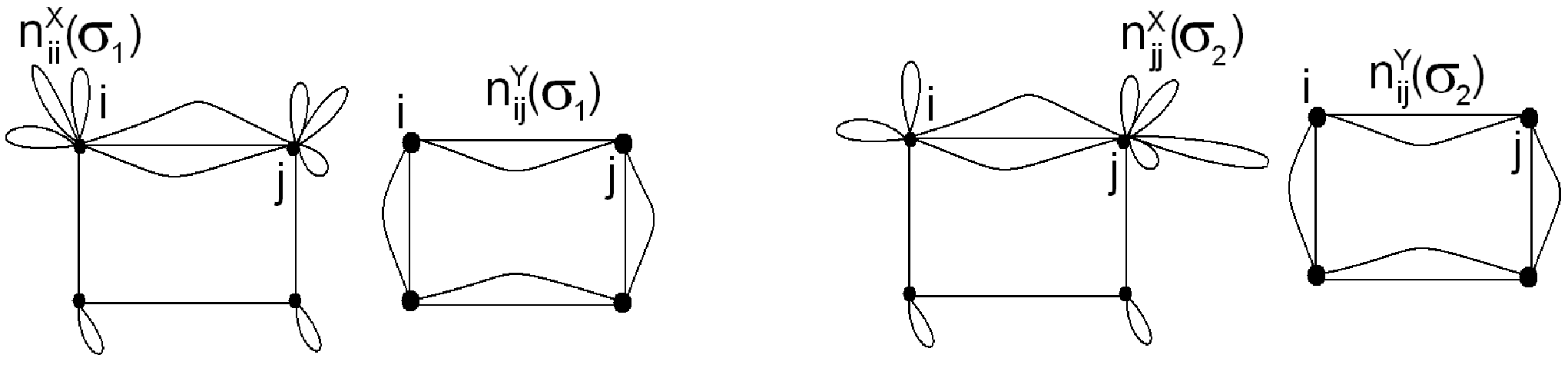
Natural hints for the construction of the Gauss operators come from the AdS/CFT correspondence. Indeed, the correspondence implies an equivalence between quantum states in the quantum gravity and operators in the 𝒩=4\mathcal{N}=4 super-Yang-Mills theory. In particular, the restricted Schur polynomials χR,(t,s,r),μ→​ν→​(X,Y,Z)\chi_{R,(t,s,r),\vec{\mu}\vec{\nu}}(X,Y,Z) are dual to multiple giant graviton systems [33, 34, 35] consisting of large branes in the A​d​S5AdS_{5} space when RR has order one rows each of length order NN, or to systems consisting of large branes in the S5S^{5} space when RR has order one columns each of length order NN. A giant graviton has a compact world volume so that the Gauss Law forces the total charge on the giant’s world volume to vanish. Since the string end points are charged, this gives a constraint on the possible open string configurations that are allowed: the number of strings leaving the giant must equal the number of strings arriving at the giant. The matrices XX and YY generate two species of 1-bit strings [36, 37, 38, 39]. Each row of RR corresponds to a giant graviton. Each open string configuration corresponds to a pair of graphs - one for each open string species. We will refer to these as the XX graph and the YY graph. The vertices of the graph represent the branes and the directed links represent the (oriented) strings. Motivated by [40] a useful combinatoric description of these graphs is to divide each string into two halves and label each half. Using the orientation of the string, label the outgoing ends with numbers {1,⋯,p}\{1,\cdots,p\} for the XX graph or {1,⋯,m}\{1,\cdots,m\} for the YY graph and the ingoing ends with these same numbers. A permutation σ∈Sp×Sm\sigma\in S_{p}\times S_{m} is then determined by how the halves are joined. We will often decompose σ=σX∘σY\sigma=\sigma^{X}\circ\sigma^{Y} with σX∈Sp\sigma^{X}\in S_{p} and σY∈Sm\sigma^{Y}\in S_{m}. Given a permutation, we can reconstruct the graphs. A graph is not associated to a unique permutation because the strings leaving the ii’th vertex are indistinguishable, and the strings arriving at the ii’th vertex are indistinguishable.

Refer to caption
Figure 1: Any open string configuration can be mapped to a pair of labeled graphs. The black graph describes the XX matrices and the red graph the YY matrices. The two bold horizontal lines are identified. The graphs determine a permutation, so each open string configuration is mapped to a permutation. For the graph shown the permutation in cycle notation is σ=(2,4)​(5,3,6)​(8,10,9)\sigma=(2,4)(5,3,6)(8,10,9). The figure shows a configuration for a three giant system with ten open strings attached. Equivalently, this is an operator whose Young diagram describing the ZZ fields has 3 long rows/columns and p=7p=7, m=3m=3. The vectors p→\vec{p} and m→\vec{m} describe the number of strings leaving each node. Thus, p→=(3,2,2)\vec{p}=(3,2,2), m→=(1,1,1)\vec{m}=(1,1,1).

We will make use of two subgroups in what follows

HY=Sm1×⋯×SmgHX=Sp1×⋯×Spg.\displaystyle H_{Y}=S_{m_{1}}\times\cdots\times S_{m_{g}}\qquad H_{X}=S_{p_{1}}\times\cdots\times S_{p_{g}}\,. (3.1)

HXH_{X} acts on boxes in the partly labeled Young diagrams that are labeled with an integer i<p+1i<p+1, i.e. on the boxes associated to XXs. HYH_{Y} acts on boxes associated to YYs. These two subgroups leave all partly labeled Young diagrams invariant. Consequently, the partly labeled Young diagrams belong to Sp×Sm/HX×HYS_{p}\times S_{m}/H_{X}\times H_{Y}. The Gauss graphs themselves are in one-to-one correspondence with elements of the double coset

HX×HY∖Sp×Sm/HX×HY\displaystyle H_{X}\times H_{Y}\setminus S_{p}\times S_{m}/H_{X}\times H_{Y} (3.2)

Introduce the states (these states span V⊗p+mV^{\otimes p+m})

|v,p→,m→⟩≡|v1⊗p1⊗v2⊗p2⊗⋯vg⊗pg⊗vg+1⊗m1⊗vg+2⊗m2⊗⋯v2​g⊗mg⟩.\displaystyle|v,\vec{p},\vec{m}\rangle\equiv|v_{1}^{\otimes p_{1}}\otimes v_{2}^{\otimes p_{2}}\otimes\cdots v_{g}^{\otimes p_{g}}\otimes v_{g+1}^{\otimes m_{1}}\otimes v_{g+2}^{\otimes m_{2}}\otimes\cdots v_{2g}^{\otimes m_{g}}\rangle\,. (3.3)

There is an action of the Sp×SmS_{p}\times S_{m} group defined on this space by

σ|vi1⊗⋯⊗vim+p⟩=|viσ⁡(1)⊗⋯⊗viσ⁡(m+p)⟩.\displaystyle\sigma|v_{i_{1}}\otimes\cdots\otimes v_{i_{m+p}}\rangle=|v_{i_{\sigma(1)}}\otimes\cdots\otimes v_{i_{\sigma(m+p)}}\rangle\,. (3.4)

This can trivially be enlarged to obtain an action of Sp+mS_{p+m}, but we want to consider only permutations that mix XX indices with each other and YY indices with each other, but not XX and YY indices. Introduce the notation |vσ⟩≡σ|v,p→,m→⟩|v_{\sigma}\rangle\equiv\sigma|v,\vec{p},\vec{m}\rangle. Invariance under the HX×HYH_{X}\times H_{Y} subgroup can be written as

|vσ⟩=|vσ​γ⟩γ∈HX×HY\displaystyle|v_{\sigma}\rangle=|v_{\sigma\gamma}\rangle\quad\gamma\in H_{X}\times H_{Y} (3.5)

or even

|vσ⟩=1|HX×HY|​∑γ∈HX×HY|vσ​γ⟩.\displaystyle|v_{\sigma}\rangle={1\over|H_{X}\times H_{Y}|}\sum_{\gamma\in H_{X}\times H_{Y}}|v_{\sigma\gamma}\rangle\,. (3.6)

Recall that the operator that projects onto representation rr of a group 𝒢{\cal G} is given by[41]

Pr=dr|𝒢|​∑g∈𝒢χr​(g)​g.\displaystyle P_{r}={d_{r}\over|{\cal G}|}\sum_{g\in{\cal G}}\chi_{r}(g)g\,. (3.7)

By the identity representation we mean the representation for which all the elements of HX×HYH_{X}\times H_{Y} are represented by 1. We want to project onto the identity representation of HX×HYH_{X}\times H_{Y} within the carrier space (s,t)(s,t) organizing the XXs and YYs. Recall that t⊢pt\vdash p and s⊢ms\vdash m. The characters in the identity representation are of course all equal to 1. The identity representation may appear more than once in (s,t)(s,t). Resolve these different copies with a multiplicity label μ→\vec{\mu}. The multiplicity label has two components, one that refers to ss and one that refers to tt. Introduce branching coefficients that resolve these projectors into a set of projectors onto each of the one dimensional spaces labeled by μ→\vec{\mu}

1|HX×HY|​∑γ∈HX×HYΓ(s,t)​(γ)i​k=∑μ→Bi​μ→(s,t)→1HX×HY​Bk​μ→s→1HX×HY.\displaystyle{1\over|H_{X}\times H_{Y}|}\sum_{\gamma\in H_{X}\times H_{Y}}\Gamma^{(s,t)}(\gamma)_{ik}=\sum_{\vec{\mu}}B^{(s,t)\to 1_{H_{X}\times H_{Y}}}_{i\vec{\mu}}B^{s\to 1_{H_{X}\times H_{Y}}}_{k\vec{\mu}}\,. (3.8)

Thus, for example, Bi​ν→(s,t)→1H​Bk​ν→(s,t)→1HB^{(s,t)\to 1_{H}}_{i\vec{\nu}}B^{(s,t)\to 1_{H}}_{k\vec{\nu}} projects onto the copy ν1\nu_{1} of the identity representation of HXH_{X} in ss and onto the copy ν2\nu_{2} of the identity representation of HYH_{Y} in tt. The branching coefficient Bi​μ→(s,t)→1HX×HYB^{(s,t)\to 1_{H_{X}\times H_{Y}}}_{i\vec{\mu}} can be understood as the one dimensional vector that spans the ν→\vec{\nu} copy of 1HX×HY1_{H_{X}\times H_{Y}} inside the carrier space of (s,t)(s,t)

|v→⟩i=Bi​ν→(s,t)→1HX×HY.\displaystyle|\vec{v}\rangle_{i}=B_{i\vec{\nu}}^{(s,t)\to 1_{H_{X}\times H_{Y}}}\,. (3.9)

Vector orthogonality says

⟨ν→|μ→⟩=δμ→​ν→=∑iBi​μ→(s,t)→1HX×HY​Bi​ν→(s,t)→1HX×HY\displaystyle\langle\vec{\nu}|\vec{\mu}\rangle=\delta_{\vec{\mu}\vec{\nu}}=\sum_{i}B^{(s,t)\to 1_{H_{X}\times H_{Y}}}_{i\vec{\mu}}B^{(s,t)\to 1_{H_{X}\times H_{Y}}}_{i\vec{\nu}} (3.10)

whilst vector completeness says

∑μ→|μ→⟩​⟨μ→|=1HX×HY\displaystyle\sum_{\vec{\mu}}|\vec{\mu}\rangle\langle\vec{\mu}|=1_{H_{X}\times H_{Y}} (3.11)

or, displaying all indices,

∑μ→Bi​μ→(s,t)→1HX×HY​Bj​μ→(s,t)→1HX×HY=(1HX×HY)i​j.\displaystyle\sum_{\vec{\mu}}B^{(s,t)\to 1_{H_{X}\times H_{Y}}}_{i\vec{\mu}}B^{(s,t)\to 1_{H_{X}\times H_{Y}}}_{j\vec{\mu}}=(1_{H_{X}\times H_{Y}})_{ij}\,. (3.12)

Together (3.10) and (3.12) allow us to think of the branching coefficients Bi​μ→(s,t)→1HX×HYB^{(s,t)\to 1_{H_{X}\times H_{Y}}}_{i\vec{\mu}} as a matrix that implements a change of basis

|i⟩=∑μ→Bi​μ→(s,t)→1HX×HY​|μ→⟩|μ→⟩=∑iBi​μ→(s,t)→1HX×HY​|i⟩.\displaystyle|i\rangle=\sum_{\vec{\mu}}B^{(s,t)\to 1_{H_{X}\times H_{Y}}}_{i\vec{\mu}}|\vec{\mu}\rangle\qquad|\vec{\mu}\rangle=\sum_{i}B^{(s,t)\to 1_{H_{X}\times H_{Y}}}_{i\vec{\mu}}|i\rangle\,. (3.13)

We are now ready to argue that the Gauss operators are simply an alternative basis to the restricted Schur polynomials. First, following [27], we will show that the number of restricted Schur polynmials is equal to the number of Gauss operators. Towards this end consider

|v(s,t),i,j⟩=∑σ∈Sm×SpΓi​j(s,t)(σ)σ|v,p→,m→⟩.\displaystyle|v_{(s,t)},i,j\rangle=\sum_{\sigma\in S_{m}\times S_{p}}\Gamma^{(s,t)}_{ij}(\sigma)\sigma|v,\vec{p},\vec{m}\rangle\,. (3.14)

Above we have projected onto the representation (s,t){(s,t)} of Sm×SpS_{m}\times S_{p}. You can think of jj as a label for different vectors and of ii as the components of the vector. According to [25] this space is organized by the Schur-Weyl duality between Sm×SpS_{m}\times S_{p} and U⁡(m)×U⁡(p)U(m)\times U(p). Concretely, we can trade the index jj for a Gelfand-Tsetlin pattern. Thus, using [25] we know that we can decompose this space as

Vg⊗p+m\displaystyle V_{g}^{\otimes p+m} =⊕c1​(s)≤g​c1​(t)≤gs⊢m​t⊢pV(s,t)U⁡(m)×U⁡(p)⊗V(s,t)Sm×Sp\displaystyle=\oplus_{{}^{s\vdash m\,\,t\vdash p}_{c_{1}(s)\leq g\,\,c_{1}(t)\leq g}}V_{(s,t)}^{U(m)\times U(p)}\otimes V_{(s,t)}^{S_{m}\times S_{p}} (3.15)
=⊕c1​(s)≤g​c1​(t)≤gs⊢m​t⊢p⊕m→​p→V(s,t)→(m→,p→)U⁡(g)×U⁡(g)→U​(1)g×U​(1)g⊗V(s,t)Sm×Sp.\displaystyle=\oplus_{{}^{s\vdash m\,\,t\vdash p}_{c_{1}(s)\leq g\,\,c_{1}(t)\leq g}}\oplus_{\vec{m}\,\,\vec{p}}V_{(s,t)\to(\vec{m},\vec{p})}^{U(g)\times U(g)\to U(1)^{g}\times U(1)^{g}}\otimes V_{(s,t)}^{S_{m}\times S_{p}}\,. (3.16)

The first factor in the last line above is the space of Gelfand-Tsetlin patterns. Now, lets consider a different decomposition of this space, as follows[27]

|v(s,t),i,j⟩\displaystyle|v_{(s,t)},i,j\rangle =∑σ∈Sm×SpΓi​j(s,t)(σ)σ|v,p→,m→⟩\displaystyle=\sum_{\sigma\in S_{m}\times S_{p}}\Gamma^{(s,t)}_{ij}(\sigma)\sigma|v,\vec{p},\vec{m}\rangle (3.21)
=∑σ∈Sm×SpΓi​j(s,t)​(σ)​|vσ⟩\displaystyle=\sum_{\sigma\in S_{m}\times S_{p}}\Gamma^{(s,t)}_{ij}(\sigma)|v_{\sigma}\rangle
=1|HX×HY|​∑σ∈Sm×Sp∑γ∈HX×HYΓ(s,t)​(σ​γ)i​j​|vσ⟩\displaystyle={1\over|H_{X}\times H_{Y}|}\sum_{\sigma\in S_{m}\times S_{p}}\sum_{\gamma\in H_{X}\times H_{Y}}\Gamma^{(s,t)}(\sigma\gamma)_{ij}|v_{\sigma}\rangle
=1|HX×HY|​∑σ∈Sm×Sp∑γ∈HX×HYΓ(s,t)​(σ)i​k​Γ(s,t)​(γ)k​j​|vσ⟩\displaystyle={1\over|H_{X}\times H_{Y}|}\sum_{\sigma\in S_{m}\times S_{p}}\sum_{\gamma\in H_{X}\times H_{Y}}\Gamma^{(s,t)}(\sigma)_{ik}\Gamma^{(s,t)}(\gamma)_{kj}|v_{\sigma}\rangle
=∑σ∈Sm×SpΓ(s,t)​(σ)i​k​∑μ→Bk​μ→(s,t)→1HX×HY​Bj​μ→(s,t)→1HX×HY​|vσ⟩.\displaystyle=\sum_{\sigma\in S_{m}\times S_{p}}\Gamma^{(s,t)}(\sigma)_{ik}\sum_{\vec{\mu}}B^{{(s,t)}\to 1_{H_{X}\times H_{Y}}}_{k\vec{\mu}}B^{{(s,t)}\to 1_{H_{X}\times H_{Y}}}_{j\vec{\mu}}|v_{\sigma}\rangle\,.

As we have already discussed, the branching coefficients provide a natural change of basis from one space to the other

|m→,p→,(s,t),μ→;i⟩=∑jBj​μ→(s,t)→1HX×HY∑σ∈Sm×SpΓi​j(s,t)(σ)σ|vσ⟩.\displaystyle|\vec{m},\vec{p},(s,t),\vec{\mu};i\rangle=\sum_{j}B_{j\vec{\mu}}^{(s,t)\to 1_{H_{X}\times H_{Y}}}\sum_{\sigma\in S_{m}\times S_{p}}\Gamma^{(s,t)}_{ij}(\sigma)\sigma|v_{\sigma}\rangle\,. (3.22)

This decomposition is[27]

Vg⊗p+m\displaystyle V_{g}^{\otimes p+m} =⊕c1​(s)≤g​c1​(t)≤gs⊢m​t⊢pV(s,t)U⁡(m)×U⁡(p)⊗V(s,t)Sm×Sp\displaystyle=\oplus_{{}^{s\vdash m\,\,t\vdash p}_{c_{1}(s)\leq g\,\,c_{1}(t)\leq g}}V_{(s,t)}^{U(m)\times U(p)}\otimes V_{(s,t)}^{S_{m}\times S_{p}} (3.23)
=⊕c1​(s)≤g​c1​(t)≤gs⊢m​t⊢p⊕m→​p→V(s,t)→1HX×HYSm×Sp→HX×HY⊗V(s,t)Sm×Sp.\displaystyle=\oplus_{{}^{s\vdash m\,\,t\vdash p}_{c_{1}(s)\leq g\,\,c_{1}(t)\leq g}}\oplus_{\vec{m}\,\,\vec{p}}V_{(s,t)\to 1_{H_{X}\times H_{Y}}}^{S_{m}\times S_{p}\to H_{X}\times H_{Y}}\otimes V_{(s,t)}^{S_{m}\times S_{p}}\,. (3.24)

Comparing (3.16) to (3.24) we conclude that

|V(s,t)→(m→,p→)U⁡(g)×U⁡(g)→U​(1)g×U​(1)g|=|V(s,t)→1HX×HYSm×Sp→HX×HY|.\displaystyle|V_{(s,t)\to(\vec{m},\vec{p})}^{U(g)\times U(g)\to U(1)^{g}\times U(1)^{g}}|=|V_{(s,t)\to 1_{H_{X}\times H_{Y}}}^{S_{m}\times S_{p}\to H_{X}\times H_{Y}}|\,. (3.25)

Using the idea that the branching coefficients provide a transformation between two bases, we easily write the Gauss operators

OR,r​(σX,σY)\displaystyle O_{R,r}(\sigma_{X},\sigma_{Y}) =|HX×HY|m!​p!​∑j​k∑s⊢m∑t⊢p∑μ→∑ν→ds​dt​Γ(s,t)​(σX∘σY)j​k\displaystyle={|H_{X}\times H_{Y}|\over\sqrt{m!p!}}\sum_{jk}\sum_{s\vdash m}\sum_{t\vdash p}\sum_{\vec{\mu}}\sum_{\vec{\nu}}\sqrt{d_{s}d_{t}}\Gamma^{(s,t)}(\sigma_{X}\circ\sigma_{Y})_{jk} (3.26)
×Bj​μ→(s,t)→1HX×HY​Bk​ν→(s,t)→1HX×HY​OR,(t,s,r)​μ→​ν→.\displaystyle\times B_{j\vec{\mu}}^{(s,t)\to 1_{H_{X}\times H_{Y}}}B_{k\vec{\nu}}^{(s,t)\to 1_{H_{X}\times H_{Y}}}O_{R,(t,s,r)\vec{\mu}\vec{\nu}}\,. (3.27)

Note that the factor ds​dt\sqrt{d_{s}d_{t}} can not be determined by group theory alone. It is chosen so that the group theoretic coefficients

Cμ→​ν→(s,t)​(σX∘σY)=|HX×HY|m!​p!​∑j​k∑s⊢m∑t⊢pds​dt​Γ(s,t)​(σX∘σY)j​k​Bj​μ→(s,t)→1HX×HY​Bk​ν→(s,t)→1HX×HY\displaystyle C^{(s,t)}_{\vec{\mu}\vec{\nu}}(\sigma_{X}\circ\sigma_{Y})={|H_{X}\times H_{Y}|\over\sqrt{m!p!}}\sum_{jk}\sum_{s\vdash m}\sum_{t\vdash p}\sqrt{d_{s}d_{t}}\Gamma^{(s,t)}(\sigma_{X}\circ\sigma_{Y})_{jk}B_{j\vec{\mu}}^{(s,t)\to 1_{H_{X}\times H_{Y}}}B_{k\vec{\nu}}^{(s,t)\to 1_{H_{X}\times H_{Y}}} (3.28)

provide an orthogonal transformation between the restricted Schur polynomials and the Gauss graph basis. Indeed,

∑(s,t)∑μ→∑ν→Cμ→​ν→(s,t)​(σX∘σY)​Cμ→​ν→(s,t)​(τX∘τY)=∑γ∈HX×HYδ⁡(γ1​σX∘σY​γ2​τX−1∘τY−1).\displaystyle\sum_{(s,t)}\sum_{\vec{\mu}}\sum_{\vec{\nu}}C^{(s,t)}_{\vec{\mu}\vec{\nu}}(\sigma_{X}\circ\sigma_{Y})C^{(s,t)}_{\vec{\mu}\vec{\nu}}(\tau_{X}\circ\tau_{Y})=\sum_{\gamma\in H_{X}\times H_{Y}}\delta(\gamma_{1}\,\sigma_{X}\circ\sigma_{Y}\,\gamma_{2}\,\tau_{X}^{-1}\circ\tau_{Y}^{-1})\,. (3.30)

There is an important point that is worth stressing here: Our Gauss operators are normalized as

⟨OR,r​(σX,σY)​OR,r​(τX,τY)†⟩=∑γ∈HX×HYδ⁡(γ1​σX∘σY​γ2​τX−1∘τY−1).\displaystyle\langle O_{R,r}(\sigma_{X},\sigma_{Y})O_{R,r}(\tau_{X},\tau_{Y})^{\dagger}\rangle=\sum_{\gamma\in H_{X}\times H_{Y}}\delta(\gamma_{1}\,\sigma_{X}\circ\sigma_{Y}\,\gamma_{2}\,\tau_{X}^{-1}\circ\tau_{Y}^{-1})\,. (3.31)

These operators certainly do not have unit two point function. For example, if we set both σX,σY\sigma_{X},\sigma_{Y} and τX,τY\tau_{X},\tau_{Y} equal to the identity permutation, the right hand side evaluates to |HX×HY||H_{X}\times H_{Y}|. Our final answer is simplest when expressed in terms of normalized operators

O^R,r​(σX,σY)≡1NσX,σY​OR,r​(σX,σY),\displaystyle\hat{O}_{R,r}(\sigma_{X},\sigma_{Y})\equiv{1\over N_{\sigma_{X},\sigma_{Y}}}O_{R,r}(\sigma_{X},\sigma_{Y})\,, (3.32)
NσX,σY2=⟨OR,r​(σX,σY)​OR,r​(σX,σY)†⟩.\displaystyle N_{\sigma_{X},\sigma_{Y}}^{2}=\langle O_{R,r}(\sigma_{X},\sigma_{Y})O_{R,r}(\sigma_{X},\sigma_{Y})^{\dagger}\rangle\,. (3.33)

We will not obtain or need the explicit form of NσX,σYN_{\sigma_{X},\sigma_{Y}}.

4 Dilatation Operator in the Gauss Graph Basis

We will now write the term in the dilatation operator that mixes XX and YY in the Gauss graph basis, i.e. we will write this term in the basis provided by (3.27). We already know that the other two terms are diagonal in this basis and we know their detailed form[25, 27].

Towards this end, transform the intertwining operator used to construct the restricted Schur polynomial

PR,(t,s,r)​μ→​ν→=∑i|m→,p→,(s,t),μ→;i⟩⟨m→,p→,(s,t),ν→;i|⊗𝟏r\displaystyle P_{R,(t,s,r)\vec{\mu}\vec{\nu}}=\sum_{i}\,\,|\vec{m},\vec{p},(s,t),\vec{\mu};i\rangle\langle\vec{m},\vec{p},(s,t),\vec{\nu};i|\otimes{\bf 1}_{r} (4.1)

to the Gauss graph basis. Of course, it is only

p(t,s)​μ→​ν→m→​p→=∑i|m→,p→,(s,t),μ→;i⟩⟨m→,p→,(s,t),ν→;i|\displaystyle p^{\vec{m}\vec{p}}_{(t,s)\vec{\mu}\vec{\nu}}=\sum_{i}\,\,|\vec{m},\vec{p},(s,t),\vec{\mu};i\rangle\langle\vec{m},\vec{p},(s,t),\vec{\nu};i| (4.2)

that we need to consider. The transformation is a simple computation

∑(s,t)|m→,p→,(s,t),μ→;i⟩⟨m→,p→,(s,t),ν→;i|Bl​ν→(s,t)→1HX×HYBm​μ→(s,t)→1HX×HYΓl​m(s,t)(σ2)\displaystyle\sum_{(s,t)}|\vec{m},\vec{p},(s,t),\vec{\mu};i\rangle\langle\vec{m},\vec{p},(s,t),\vec{\nu};i|B_{l\vec{\nu}}^{(s,t)\to 1_{H_{X}\times H_{Y}}}B_{m\vec{\mu}}^{(s,t)\to 1_{H_{X}\times H_{Y}}}\Gamma_{lm}^{(s,t)}(\sigma_{2}) (4.3)
=1|HX×HY|​m!​p!​∑(s,t)∑σ,τ∈Sm×Spds​dt​Bj​μ→(s,t)→1HX×HY​Γb​j(s,t)​(σ)​|vσ⟩​⟨vτ|​Γb​k(s,t)​(τ)​Bk​ν→(s,t)→1HX×HY\displaystyle={1\over|H_{X}\times H_{Y}|m!p!}\sum_{(s,t)}\sum_{\sigma,\tau\in S_{m}\times S_{p}}d_{s}d_{t}~~B^{(s,t)\to 1_{H_{X}\times H_{Y}}}_{j\vec{\mu}}\Gamma^{(s,t)}_{bj}(\sigma)|v_{\sigma}\rangle\langle v_{\tau}|\Gamma^{(s,t)}_{bk}(\tau)B^{(s,t)\to 1_{H_{X}\times H_{Y}}}_{k\vec{\nu}} (4.4)
×Bl​ν→(s,t)→1HX×HY​Bm​μ→(s,t)→1HX×HY​Γl​m(s,t)​(σ2)\displaystyle\qquad\times B_{l\vec{\nu}}^{(s,t)\to 1_{H_{X}\times H_{Y}}}B_{m\vec{\mu}}^{(s,t)\to 1_{H_{X}\times H_{Y}}}\Gamma_{lm}^{(s,t)}(\sigma_{2}) (4.5)
=1|HX×HY|​m!​p!​∑(s,t)∑σ,τ∈Sm×Spds​dt​|vσ⟩​⟨vτ|​Γj​k(s,t)​(σ−1​τ)​Bj​μ→(s,t)→1HX×HY​Bk​ν→(s,t)→1HX×HY\displaystyle={1\over|H_{X}\times H_{Y}|m!p!}\sum_{(s,t)}\sum_{\sigma,\tau\in S_{m}\times S_{p}}d_{s}d_{t}~~|v_{\sigma}\rangle\langle v_{\tau}|\Gamma^{(s,t)}_{jk}(\sigma^{-1}\tau)B^{(s,t)\to 1_{H_{X}\times H_{Y}}}_{j\vec{\mu}}B^{(s,t)\to 1_{H_{X}\times H_{Y}}}_{k\vec{\nu}} (4.6)
Bl​ν→(s,t)→1HX×HY​Bm​μ→(s,t)→1HX×HY​Γl​m​(σ2)\displaystyle\qquad B^{(s,t)\to 1_{H_{X}\times H_{Y}}}_{l\vec{\nu}}B^{(s,t)\to 1_{H_{X}\times H_{Y}}}_{m\vec{\mu}}\Gamma_{lm}(\sigma_{2}) (4.7)
=1|HX×HY|​m!​p!​∑(s,t)∑σ,τ∈Sm×Sp1|HX×HY|2​∑γ1,γ2∈HX×HYds​dt​Γj​m(s,t)​(γ1)​Γk​l(s,t)​(γ2)​Γl​m(s,t)​(σ2)\displaystyle={1\over|H_{X}\times H_{Y}|m!p!}\sum_{(s,t)}\sum_{\sigma,\tau\in S_{m}\times S_{p}}{1\over|H_{X}\times H_{Y}|^{2}}\sum_{\gamma_{1},\gamma_{2}\in H_{X}\times H_{Y}}d_{s}d_{t}\Gamma_{jm}^{(s,t)}(\gamma_{1})\Gamma_{kl}^{(s,t)}(\gamma_{2})\Gamma_{lm}^{(s,t)}(\sigma_{2}) (4.8)
×Γj​k(s,t)​(σ−1​τ)​|vσ⟩​⟨vτ|\displaystyle\qquad\times\Gamma_{jk}^{(s,t)}(\sigma^{-1}\tau)|v_{\sigma}\rangle\langle v_{\tau}| (4.9)
=1m!​p!​|HX×HY|​∑(s,t)∑σ,τ∈Sm×Sp1|HX×HY|2​∑γ1,γ2∈HX×HYds​dt​χu​(γ1​σ2−1​γ2−1​τ−1​σ)​|vσ⟩​⟨vτ|\displaystyle={1\over m!p!|H_{X}\times H_{Y}|}\sum_{(s,t)}\sum_{\sigma,\tau\in S_{m}\times S_{p}}{1\over|H_{X}\times H_{Y}|^{2}}\sum_{\gamma_{1},\gamma_{2}\in H_{X}\times H_{Y}}d_{s}d_{t}\chi_{u}(\gamma_{1}\sigma_{2}^{-1}\gamma_{2}^{-1}\tau^{-1}\sigma)|v_{\sigma}\rangle\langle v_{\tau}| (4.10)
=1|HX×HY|3​∑σ,τ∈Sm×Sp∑γ1,γ2∈HX×HYδ⁡(γ1​σ2−1​γ2−1​τ−1​σ)​|vσ⟩​⟨vτ|.\displaystyle={1\over|H_{X}\times H_{Y}|^{3}}\sum_{\sigma,\tau\in S_{m}\times S_{p}}\sum_{\gamma_{1},\gamma_{2}\in H_{X}\times H_{Y}}\delta(\gamma_{1}\sigma_{2}^{-1}\gamma_{2}^{-1}\tau^{-1}\sigma)|v_{\sigma}\rangle\langle v_{\tau}|\,. (4.11)

Notice that up to normalization this is a sum over all σ,τ∈Sm×Sp\sigma,\tau\in S_{m}\times S_{p} of |vσ⟩​⟨vτ||v_{\sigma}\rangle\langle v_{\tau}| with the condition that τ−1​σ\tau^{-1}\sigma belongs to the same coset as σ2\sigma_{2} does. With this result in hand, we easily find

⟨OT,w†​(σ2)​DX​Y​OR,r​(σ1)⟩=\displaystyle\langle O^{\dagger}_{T,w}(\sigma_{2})D_{XY}O_{R,r}(\sigma_{1})\rangle\qquad\qquad= (4.12)
=|HX×HY|​|HX′×HY′|m!​p!​∑j​k∑s⊢m∑t⊢p∑μ→​ν→∑l​m∑x⊢m∑y⊢p∑α→​β→ds​dt​dx​dy​Γ(s,t)​(σ1)j​k​Γ(x,y)​(σ2)l​m\displaystyle={|H_{X}\times H_{Y}||H^{\prime}_{X}\times H^{\prime}_{Y}|\over m!p!}\sum_{jk}\sum_{s\vdash m}\sum_{t\vdash p}\sum_{\vec{\mu}\vec{\nu}}\sum_{lm}\sum_{x\vdash m}\sum_{y\vdash p}\sum_{\vec{\alpha}\vec{\beta}}\sqrt{d_{s}d_{t}}\sqrt{d_{x}d_{y}}\Gamma^{(s,t)}(\sigma_{1})_{jk}\Gamma^{(x,y)}(\sigma_{2})_{lm} (4.13)
×Bj​μ→(s,t)→1HX×HY​Bk​ν→(s,t)→1HX×HY​Bl​α→(x,y)→1HX′×HY′​Bm​β→(x,y)→1HX′×HY′​⟨OT,(y,x,w)​α→​β→†​DX​Y​OR,(t,s,r)​μ→​ν→⟩\displaystyle\times B^{(s,t)\to 1_{H_{X}\times H_{Y}}}_{j\vec{\mu}}B^{(s,t)\to 1_{H_{X}\times H_{Y}}}_{k\vec{\nu}}B^{(x,y)\to 1_{H^{\prime}_{X}\times H^{\prime}_{Y}}}_{l\vec{\alpha}}B^{(x,y)\to 1_{H^{\prime}_{X}\times H^{\prime}_{Y}}}_{m\vec{\beta}}\langle O^{\dagger}_{T,(y,x,w)\vec{\alpha}\vec{\beta}}D_{XY}O_{R,(t,s,r)\vec{\mu}\vec{\nu}}\rangle (4.14)
(4.15)
=|HX×HY|​|HX′×HY′|m!​p!​∑j​k∑s⊢m∑t⊢p∑μ→​ν→∑l​m∑x⊢m∑y⊢p∑α→​β→ds​dt​dx​dy​Γ(s,t)​(σ1)j​k​Γ(x,y)​(σ2)l​m\displaystyle={|H_{X}\times H_{Y}||H^{\prime}_{X}\times H^{\prime}_{Y}|\over m!p!}\sum_{jk}\sum_{s\vdash m}\sum_{t\vdash p}\sum_{\vec{\mu}\vec{\nu}}\sum_{lm}\sum_{x\vdash m}\sum_{y\vdash p}\sum_{\vec{\alpha}\vec{\beta}}\sqrt{d_{s}d_{t}}\sqrt{d_{x}d_{y}}\Gamma^{(s,t)}(\sigma_{1})_{jk}\Gamma^{(x,y)}(\sigma_{2})_{lm} (4.16)
×Bj​μ→(s,t)→1HX×HY​Bk​ν→(s,t)→1HX×HY​Bl​α→(x,y)→1HX′×HY′​Bm​β→(x,y)→1HX′×HY′\displaystyle\times B^{(s,t)\to 1_{H_{X}\times H_{Y}}}_{j\vec{\mu}}B^{(s,t)\to 1_{H_{X}\times H_{Y}}}_{k\vec{\nu}}B^{(x,y)\to 1_{H^{\prime}_{X}\times H^{\prime}_{Y}}}_{l\vec{\alpha}}B^{(x,y)\to 1_{H^{\prime}_{X}\times H^{\prime}_{Y}}}_{m\vec{\beta}} (4.17)
×∑R′cR​R′​dT​m​pdx​dy​(n+m+p)​dR′​fT​hooksT​hookss​hookstfR​hooksR​hooksx​hooksy​δr​w\displaystyle\times\sum_{R^{\prime}}c_{RR^{\prime}}{d_{T}mp\over d_{x}d_{y}(n+m+p)d_{R^{\prime}}}\sqrt{f_{T}{\rm hooks}_{T}{\rm hooks}_{s}{\rm hooks}_{t}\over f_{R}{\rm hooks}_{R}{\rm hooks}_{x}{\rm hooks}_{y}}\delta_{rw} (4.18)
×(⟨p→,t,ν1;a​|El​j(1)|​p→′,y,α1;b⟩​⟨p→′,y,β1;b​|Ek​i(1)|​p→,t,μ1;a⟩CLOSE\displaystyle\times\Big(\langle\vec{p},t,\nu_{1};a|E^{(1)}_{lj}|\vec{p}^{\prime},y,\alpha_{1};b\rangle\langle\vec{p}^{\prime},y,\beta_{1};b|E^{(1)}_{ki}|\vec{p},t,\mu_{1};a\rangle (4.19)
×⟨m→,s,ν2;c​|Ei​l(p+1)|​m→′,x,α2;d⟩​⟨m→′,x,β2;d​|Ej​k(p+1)|​m→,s,μ2;c⟩\displaystyle\qquad\times\langle\vec{m},s,\nu_{2};c|E^{(p+1)}_{il}|\vec{m}^{\prime},x,\alpha_{2};d\rangle\langle\vec{m}^{\prime},x,\beta_{2};d|E^{(p+1)}_{jk}|\vec{m},s,\mu_{2};c\rangle (4.20)
−δp→​p→′​δy​t​δν1​α1​δm→​m→′​δs​x​δβ2​μ2​⟨p→′,y,β1;b​|Ej​i(1)|​p→,t,μ1;a⟩​⟨m→,s,ν2;c​|Ei​j(p+1)|​m→′,x,α2;d⟩\displaystyle-\delta_{\vec{p}\vec{p}^{\prime}}\delta_{yt}\delta_{\nu_{1}\alpha_{1}}\delta_{\vec{m}\vec{m}^{\prime}}\delta_{sx}\delta_{\beta_{2}\mu_{2}}\langle\vec{p}^{\prime},y,\beta_{1};b|E^{(1)}_{ji}|\vec{p},t,\mu_{1};a\rangle\langle\vec{m},s,\nu_{2};c|E^{(p+1)}_{ij}|\vec{m}^{\prime},x,\alpha_{2};d\rangle (4.21)
−δp→​p→′​δy​t​δμ1​β1​δm→​m→′​δs​x​δα2​ν2​⟨p→,t,ν1;a​|Ei​j(1)|​p→′,y,α1;b⟩​⟨m→′,x,β2;d​|Ej​i(p+1)|​m→,s,μ2;c⟩\displaystyle-\delta_{\vec{p}\vec{p}^{\prime}}\delta_{yt}\delta_{\mu_{1}\beta_{1}}\delta_{\vec{m}\vec{m}^{\prime}}\delta_{sx}\delta_{\alpha_{2}\nu_{2}}\langle\vec{p},t,\nu_{1};a|E^{(1)}_{ij}|\vec{p}^{\prime},y,\alpha_{1};b\rangle\langle\vec{m}^{\prime},x,\beta_{2};d|E^{(p+1)}_{ji}|\vec{m},s,\mu_{2};c\rangle (4.22)
+⟨p→,t,ν1;a​|Ei​l(1)|​p→′,y,α1;b⟩​⟨p→′,y,β1;b​|Ej​k(1)|​p→,t,μ1;a⟩\displaystyle+\langle\vec{p},t,\nu_{1};a|E^{(1)}_{il}|\vec{p}^{\prime},y,\alpha_{1};b\rangle\langle\vec{p}^{\prime},y,\beta_{1};b|E^{(1)}_{jk}|\vec{p},t,\mu_{1};a\rangle (4.23)
×⟨m→,s,ν2;c|El​j(p+1)|m→′,x,α2;d⟩⟨m→′,x,β2;d|Ek​i(p+1)|m→,s,μ2;c⟩)\displaystyle\qquad\times\langle\vec{m},s,\nu_{2};c|E^{(p+1)}_{lj}|\vec{m}^{\prime},x,\alpha_{2};d\rangle\langle\vec{m}^{\prime},x,\beta_{2};d|E^{(p+1)}_{ki}|\vec{m},s,\mu_{2};c\rangle\Big) (4.24)
(4.25)
=|HX×HY|​|HX′×HY′|m!​p!​∑j​k∑s⊢m∑t⊢p∑μ→​ν→∑l​m∑x⊢m∑y⊢p∑α→​β→Γ(s,t)​(σ1)j​k​Γ(x,y)​(σ2)l​m\displaystyle={|H_{X}\times H_{Y}||H^{\prime}_{X}\times H^{\prime}_{Y}|\over m!p!}\sum_{jk}\sum_{s\vdash m}\sum_{t\vdash p}\sum_{\vec{\mu}\vec{\nu}}\sum_{lm}\sum_{x\vdash m}\sum_{y\vdash p}\sum_{\vec{\alpha}\vec{\beta}}\Gamma^{(s,t)}(\sigma_{1})_{jk}\Gamma^{(x,y)}(\sigma_{2})_{lm} (4.26)
×Bj​μ→(s,t)→1HX×HY​Bk​ν→(s,t)→1HX×HY​Bl​α→(x,y)→1HX′×HY′​Bm​β→(x,y)→1HX′×HY′\displaystyle\times B^{(s,t)\to 1_{H_{X}\times H_{Y}}}_{j\vec{\mu}}B^{(s,t)\to 1_{H_{X}\times H_{Y}}}_{k\vec{\nu}}B^{(x,y)\to 1_{H^{\prime}_{X}\times H^{\prime}_{Y}}}_{l\vec{\alpha}}B^{(x,y)\to 1_{H^{\prime}_{X}\times H^{\prime}_{Y}}}_{m\vec{\beta}} (4.27)
∑R′cR​R′​dT​m​p(n+m+p)​dR′​fT​hooksTfR​hooksR​δr​w​(⟨p→,t,ν1;a​|El​j(1)|​p→′,y,α1;b⟩​⟨p→′,y,β1;b​|Ek​i(1)|​p→,t,μ1;a⟩CLOSE\displaystyle\sum_{R^{\prime}}c_{RR^{\prime}}{d_{T}mp\over(n+m+p)d_{R^{\prime}}}\sqrt{f_{T}{\rm hooks}_{T}\over f_{R}{\rm hooks}_{R}}\delta_{rw}\Big(\langle\vec{p},t,\nu_{1};a|E^{(1)}_{lj}|\vec{p}^{\prime},y,\alpha_{1};b\rangle\langle\vec{p}^{\prime},y,\beta_{1};b|E^{(1)}_{ki}|\vec{p},t,\mu_{1};a\rangle (4.28)
×⟨m→,s,ν2;c​|Ei​l(p+1)|​m→′,x,α2;d⟩​⟨m→′,x,β2;d​|Ej​k(p+1)|​m→,s,μ2;c⟩\displaystyle\qquad\times\langle\vec{m},s,\nu_{2};c|E^{(p+1)}_{il}|\vec{m}^{\prime},x,\alpha_{2};d\rangle\langle\vec{m}^{\prime},x,\beta_{2};d|E^{(p+1)}_{jk}|\vec{m},s,\mu_{2};c\rangle (4.29)
−δp→​p→′​δy​t​δν1​α1​δm→​m→′​δs​x​δβ2​μ2​⟨p→′,y,β1;b​|Ej​i(1)|​p→,t,μ1;a⟩​⟨m→,s,ν2;c​|Ei​j(p+1)|​m→′,x,α2;d⟩\displaystyle-\delta_{\vec{p}\vec{p}^{\prime}}\delta_{yt}\delta_{\nu_{1}\alpha_{1}}\delta_{\vec{m}\vec{m}^{\prime}}\delta_{sx}\delta_{\beta_{2}\mu_{2}}\langle\vec{p}^{\prime},y,\beta_{1};b|E^{(1)}_{ji}|\vec{p},t,\mu_{1};a\rangle\langle\vec{m},s,\nu_{2};c|E^{(p+1)}_{ij}|\vec{m}^{\prime},x,\alpha_{2};d\rangle (4.30)
−δp→​p→′​δy​t​δμ1​β1​δm→​m→′​δs​x​δα2​ν2​⟨p→,t,ν1;a​|Ei​j(1)|​p→′,y,α1;b⟩​⟨m→′,x,β2;d​|Ej​i(p+1)|​m→,s,μ2;c⟩\displaystyle-\delta_{\vec{p}\vec{p}^{\prime}}\delta_{yt}\delta_{\mu_{1}\beta_{1}}\delta_{\vec{m}\vec{m}^{\prime}}\delta_{sx}\delta_{\alpha_{2}\nu_{2}}\langle\vec{p},t,\nu_{1};a|E^{(1)}_{ij}|\vec{p}^{\prime},y,\alpha_{1};b\rangle\langle\vec{m}^{\prime},x,\beta_{2};d|E^{(p+1)}_{ji}|\vec{m},s,\mu_{2};c\rangle (4.31)
+⟨p→,t,ν1;a​|Ei​l(1)|​p→′,y,α1;b⟩​⟨p→′,y,β1;b​|Ej​k(1)|​p→,t,μ1;a⟩\displaystyle+\langle\vec{p},t,\nu_{1};a|E^{(1)}_{il}|\vec{p}^{\prime},y,\alpha_{1};b\rangle\langle\vec{p}^{\prime},y,\beta_{1};b|E^{(1)}_{jk}|\vec{p},t,\mu_{1};a\rangle (4.32)
×⟨m→,s,ν2;c|El​j(p+1)|m→′,x,α2;d⟩⟨m→′,x,β2;d|Ek​i(p+1)|m→,s,μ2;c⟩).\displaystyle\qquad\times\langle\vec{m},s,\nu_{2};c|E^{(p+1)}_{lj}|\vec{m}^{\prime},x,\alpha_{2};d\rangle\langle\vec{m}^{\prime},x,\beta_{2};d|E^{(p+1)}_{ki}|\vec{m},s,\mu_{2};c\rangle\Big)\,.

There are four terms in the above expression. We will deal with each term, one at a time.

4.1 First term

Focus on the first term for now

=|HX×HY|​|HX′×HY′|m!​p!​∑j​k∑s⊢m∑t⊢p∑μ→​ν→∑l​m∑x⊢m∑y⊢p∑α→​β→Γ(s,t)​(σ1)j​k​Γ(x,y)​(σ2)l​m\displaystyle={|H_{X}\times H_{Y}||H^{\prime}_{X}\times H^{\prime}_{Y}|\over m!p!}\sum_{jk}\sum_{s\vdash m}\sum_{t\vdash p}\sum_{\vec{\mu}\vec{\nu}}\sum_{lm}\sum_{x\vdash m}\sum_{y\vdash p}\sum_{\vec{\alpha}\vec{\beta}}\Gamma^{(s,t)}(\sigma_{1})_{jk}\Gamma^{(x,y)}(\sigma_{2})_{lm} (4.33)
×Bj​μ→(s,t)→1HX×HY​Bk​ν→(s,t)→1HX×HY​Bl​α→(x,y)→1HX′×HY′​Bm​β→(x,y)→1HX′×HY′\displaystyle\times B^{(s,t)\to 1_{H_{X}\times H_{Y}}}_{j\vec{\mu}}B^{(s,t)\to 1_{H_{X}\times H_{Y}}}_{k\vec{\nu}}B^{(x,y)\to 1_{H^{\prime}_{X}\times H^{\prime}_{Y}}}_{l\vec{\alpha}}B^{(x,y)\to 1_{H^{\prime}_{X}\times H^{\prime}_{Y}}}_{m\vec{\beta}} (4.34)
∑R′cR​R′​dT​m​p(n+m+p)​dR′​fT​hooksTfR​hooksR​δr​w​⟨p→,t,ν1;a​|El​j(1)|​p→′,y,α1;b⟩​⟨p→′,y,β1;b​|Ek​i(1)|​p→,t,μ1;a⟩\displaystyle\sum_{R^{\prime}}c_{RR^{\prime}}{d_{T}mp\over(n+m+p)d_{R^{\prime}}}\sqrt{f_{T}{\rm hooks}_{T}\over f_{R}{\rm hooks}_{R}}\delta_{rw}\langle\vec{p},t,\nu_{1};a|E^{(1)}_{lj}|\vec{p}^{\prime},y,\alpha_{1};b\rangle\langle\vec{p}^{\prime},y,\beta_{1};b|E^{(1)}_{ki}|\vec{p},t,\mu_{1};a\rangle (4.35)
×⟨m→,s,ν2;c​|Ei​l(p+1)|​m→′,x,α2;d⟩​⟨m→′,x,β2;d​|Ej​k(p+1)|​m→,s,μ2;c⟩\displaystyle\hskip 18.49988pt\times\langle\vec{m},s,\nu_{2};c|E^{(p+1)}_{il}|\vec{m}^{\prime},x,\alpha_{2};d\rangle\langle\vec{m}^{\prime},x,\beta_{2};d|E^{(p+1)}_{jk}|\vec{m},s,\mu_{2};c\rangle (4.36)
=1|HX×HY|2​|HX′×HY′|2​m!​p!\displaystyle={1\over|H_{X}\times H_{Y}|^{2}|H^{\prime}_{X}\times H^{\prime}_{Y}|^{2}m!p!} (4.37)
∑R′cR​R′hooksR′mpfTfR​hooksR​hooksTδr​w∑τ∈Sm×Sp∑ϕ∈Sm×Sp∑γ1,γ2∈HX′×HY′∑β1,β2∈HX×HY\displaystyle\sum_{R^{\prime}}c_{RR^{\prime}}{\rm hooks}_{R^{\prime}}mp\sqrt{f_{T}\over f_{R}{\rm hooks}_{R}{\rm hooks}_{T}}\delta_{rw}\sum_{\tau\in S_{m}\times S_{p}}\sum_{\phi\in S_{m}\times S_{p}}\sum_{\gamma_{1},\gamma_{2}\in H_{X}^{\prime}\times H_{Y}^{\prime}}\sum_{\beta_{1},\beta_{2}\in H_{X}\times H_{Y}} (4.38)
×⟨v,p→′,m→′​|Ej​iτ−1​(p+1)​τ−1​(1,p+1)​ϕ​β2​σ2​β1−1|​v,p→,m→⟩​⟨v,p→,m→​|Ei​jϕ−1​(p+1)​ϕ−1​(1,p+1)​τ​γ2​σ1​γ1−1|​v,p→′,m→′⟩\displaystyle\times\langle v,\vec{p}^{\prime},\vec{m}^{\prime}|E^{\tau^{-1}(p+1)}_{ji}\tau^{-1}\,(1,p+1)\,\phi\beta_{2}\sigma_{2}\beta_{1}^{-1}|v,\vec{p},\vec{m}\rangle\langle v,\vec{p},\vec{m}|E^{\phi^{-1}(p+1)}_{ij}\phi^{-1}\,(1,p+1)\,\tau\gamma_{2}\sigma_{1}\gamma_{1}^{-1}|v,\vec{p}^{\prime},\vec{m}^{\prime}\rangle

Now, lets study the case that i=ji=j. To find a simple condition on p→′,m→′\vec{p}^{\prime},\vec{m}^{\prime} and p→,m→\vec{p},\vec{m} that tells us when this matrix element is non-zero, focus on

⟨vτ|Ej​i(p+1)​(1,p+1)|vψ⟩​⟨vϕ|(1,p+1)​Ei​j(1)|vσ⟩.\displaystyle\langle v_{\tau}|E^{(p+1)}_{ji}\,(1,p+1)\,|v_{\psi}\rangle\langle v_{\phi}|\,(1,p+1)\,E^{(1)}_{ij}|v_{\sigma}\rangle\,. (4.39)

If i=ji=j, the matrix element ⟨v,p→′,m→′​|τ−1​Ej​i(p+1)​(1,p+1)​ψ|​v,p→,m→⟩\langle v,\vec{p}^{\prime},\vec{m}^{\prime}|\tau^{-1}E^{(p+1)}_{ji}\,(1,p+1)\,\psi|v,\vec{p},\vec{m}\rangle forces p→+m→=p→′+m→′\vec{p}+\vec{m}=\vec{p}^{\prime}+\vec{m}^{\prime}. Indeed, Ei​i(p+1)E^{(p+1)}_{ii} is one if the vector in the first slot of ψ|v,p→,m→⟩\psi|v,\vec{p},\vec{m}\rangle is v1v_{1} and it is zero otherwise, so it clearly does not change the identity of any vectors. The remaining elements between the two states (i.e. τ−1\tau^{-1} and (1,p+1)​ψ(1,p+1)\,\psi) can swap vectors around but not change the identity of any vector. Thus, the identity of the collection of vectors used to construct |v,p→,m→⟩|v,\vec{p},\vec{m}\rangle must match the identity of the collection of vectors used to construct |v,p→′,m→′⟩|v,\vec{p}^{\prime},\vec{m}^{\prime}\rangle. This then proves that p→+m→=p→′+m→′\vec{p}+\vec{m}=\vec{p}^{\prime}+\vec{m}^{\prime}. We can argue for this conclusion in a second way: recall that we obtain R′R^{\prime} from RR by dropping box in row ii and we obtain T′T^{\prime} from TT by dropping a box in row jj. Thus, if i=ji=j, since R′=T′R^{\prime}=T^{\prime} we are saying that R=TR=T. We already know that r=wr=w. p→+m→\vec{p}+\vec{m} tells us the collection of boxes that needs to be dropped from RR to get rr and p→′+m→′\vec{p}^{\prime}+\vec{m}^{\prime} tells us the collection of boxes that needs to be dropped from TT to get ww. Since R=TR=T and r=wr=w, this then again proves that p→+m→=p→′+m→′\vec{p}+\vec{m}=\vec{p}^{\prime}+\vec{m}^{\prime}. We can say a bit more. Consider

⟨v,p→,m→​|ϕ−1​(1,p+1)​Ei​i(1)​σ|​v,p→′,m→′⟩.\displaystyle\langle v,\vec{p},\vec{m}|\phi^{-1}\,(1,p+1)\,E^{(1)}_{ii}\sigma|v,\vec{p}^{\prime},\vec{m}^{\prime}\rangle\,. (4.40)

This tells you that if you take the state |v,p→′,m→′⟩|v,\vec{p}^{\prime},\vec{m}^{\prime}\rangle and shuffle some of the XX slots amongst each other and some of the YY slots amongst each other (σ\sigma does this shuffling) keeping only states with vector viv_{i} in their first slot, and then swapping the vectors in slots 11 and p+1p+1, we can get the vector |v,p→,m→⟩|v,\vec{p},\vec{m}\rangle by shuffling (according to ϕ−1\phi^{-1}) what we have. Thus, to get |v,p→,m→⟩|v,\vec{p},\vec{m}\rangle from |v,p→′,m→′⟩|v,\vec{p}^{\prime},\vec{m}^{\prime}\rangle we removed viv_{i} from an XX slot of |v,p→′,m→′⟩|v,\vec{p}^{\prime},\vec{m}^{\prime}\rangle and inserted it into a YY slot of |v,p→,m→⟩|v,\vec{p},\vec{m}\rangle.

Now consider

⟨v,p→′,m→′​|τ−1​Ei​i(p+1)​(1,p+1)​ψ|​v,p→,m→⟩.\displaystyle\langle v,\vec{p}^{\prime},\vec{m}^{\prime}|\tau^{-1}E^{(p+1)}_{ii}\,(1,p+1)\psi|v,\vec{p},\vec{m}\rangle\,. (4.41)

This tells you that if you take the state |v,p→,m→⟩|v,\vec{p},\vec{m}\rangle and shuffle some of the XX slots amongst each other and some of the YY slots amongst each other (ψ\psi does this shuffling) keeping only states with vector viv_{i} in their first slot, and then, swapping the vectors in slots 11 and p+1p+1, we can get the vector |v,p→′,m→′⟩|v,\vec{p}^{\prime},\vec{m}^{\prime}\rangle by shuffling (according to τ−1\tau^{-1}) what we have. Thus, to get |v,p→′,m→′⟩|v,\vec{p}^{\prime},\vec{m}^{\prime}\rangle from |v,p→,m→⟩|v,\vec{p},\vec{m}\rangle we removed viv_{i} from an XX slot of |v,p→,m→⟩|v,\vec{p},\vec{m}\rangle and inserted it into a YY slot of |v,p→,m→⟩|v,\vec{p},\vec{m}\rangle.

Thus, the two vectors we are swapping have the same identity. This implies that we must have p→=p→′\vec{p}=\vec{p}^{\prime} and m→=m→′\vec{m}=\vec{m}^{\prime}. Since we must have p→=p→′\vec{p}=\vec{p}^{\prime} and m→=m→′\vec{m}=\vec{m}^{\prime} we find

=1|HX×HY|4​m!​p!∑R′cR​R′hooksR′mpfTfR​hooksR​hooksTδr​w∑τ∈Sm×Sp∑ϕ∈Sm×Sp∑γ1,γ2,β1,β2∈HX×HY\displaystyle={1\over|H_{X}\times H_{Y}|^{4}m!p!}\sum_{R^{\prime}}c_{RR^{\prime}}{\rm hooks}_{R^{\prime}}mp\sqrt{f_{T}\over f_{R}{\rm hooks}_{R}{\rm hooks}_{T}}\delta_{rw}\sum_{\tau\in S_{m}\times S_{p}}\sum_{\phi\in S_{m}\times S_{p}}\sum_{\gamma_{1},\gamma_{2},\beta_{1},\beta_{2}\in H_{X}\times H_{Y}} (4.42)
×⟨v,p→,m→​|Ej​iτ−1​(p+1)​τ−1​(1,p+1)​ϕ​β2​σ2​β1−1|​v,p→,m→⟩​⟨v,p→,m→​|Ei​jϕ−1​(p+1)​ϕ−1​(1,p+1)​τ​γ2​σ1​γ1−1|​v,p→,m→⟩\displaystyle\times\langle v,\vec{p},\vec{m}|E^{\tau^{-1}(p+1)}_{ji}\tau^{-1}\,(1,p+1)\,\phi\beta_{2}\sigma_{2}\beta_{1}^{-1}|v,\vec{p},\vec{m}\rangle\langle v,\vec{p},\vec{m}|E^{\phi^{-1}(p+1)}_{ij}\phi^{-1}\,(1,p+1)\,\tau\gamma_{2}\sigma_{1}\gamma_{1}^{-1}|v,\vec{p},\vec{m}\rangle (4.43)
=1|HX×HY|4​m!​p!∑R′cR​R′hooksR′mpfTfR​hooksR​hooksTδr​w∑τ∈Sm×Sp∑ϕ∈Sm×Sp∑γ1,γ2,β1,β2,ρ1,ρ2∈HX×HY\displaystyle={1\over|H_{X}\times H_{Y}|^{4}m!p!}\sum_{R^{\prime}}c_{RR^{\prime}}{\rm hooks}_{R^{\prime}}mp\sqrt{f_{T}\over f_{R}{\rm hooks}_{R}{\rm hooks}_{T}}\delta_{rw}\sum_{\tau\in S_{m}\times S_{p}}\sum_{\phi\in S_{m}\times S_{p}}\sum_{\gamma_{1},\gamma_{2},\beta_{1},\beta_{2},\rho_{1},\rho_{2}\in H_{X}\times H_{Y}} (4.44)
×δ⁡(τ−1​ϕ​β2​σ2​β1−1​ρ1)​δ​(ϕ−1​τ​γ2​σ1​γ1−1​ρ2)\displaystyle\times\delta(\tau^{-1}\,\phi\beta_{2}\sigma_{2}\beta_{1}^{-1}\rho_{1})\delta(\phi^{-1}\,\tau\gamma_{2}\sigma_{1}\gamma_{1}^{-1}\rho_{2}) (4.45)
×∑k,q∈Si,m∑l,r∈Si,pδ⁡(τ−1​(p+1),k)​δ​(τ−1​(1),l)​δ​(ϕ−1​(p+1),q)​δ​(ϕ−1​(1),r).\displaystyle\times\sum_{k,q\in S_{i,m}}\sum_{l,r\in S_{i,p}}\delta(\tau^{-1}(p+1),k)\delta(\tau^{-1}(1),l)\delta(\phi^{-1}(p+1),q)\delta(\phi^{-1}(1),r)\,.

Now, set τ=α​τ~\tau=\alpha\tilde{\tau} and β=α​β~\beta=\alpha\tilde{\beta} with α∈Zm×Zp\alpha\in Z_{m}\times Z_{p}, with Zm×ZpZ_{m}\times Z_{p} a product of cyclic groups. The above expression becomes

=1|HX×HY|4​m!​p!∑R′cR​R′hooksR′mpfTfR​hooksR​hooksTδr​w∑τ∈Sm×Sp∑ϕ∈Sm×Sp\displaystyle={1\over|H_{X}\times H_{Y}|^{4}m!p!}\sum_{R^{\prime}}c_{RR^{\prime}}{\rm hooks}_{R^{\prime}}mp\sqrt{f_{T}\over f_{R}{\rm hooks}_{R}{\rm hooks}_{T}}\delta_{rw}\sum_{\tau\in S_{m}\times S_{p}}\sum_{\phi\in S_{m}\times S_{p}} (4.46)
×∑γ1,γ2,β1,β2,ρ1,ρ2∈HX×HYδ⁡(τ−1​ϕ​β2​σ2​β1−1​ρ1)​δ​(ϕ−1​τ​γ2​σ1​γ1−1​ρ2)\displaystyle\times\sum_{\gamma_{1},\gamma_{2},\beta_{1},\beta_{2},\rho_{1},\rho_{2}\in H_{X}\times H_{Y}}\delta(\tau^{-1}\,\phi\beta_{2}\sigma_{2}\beta_{1}^{-1}\rho_{1})\delta(\phi^{-1}\,\tau\gamma_{2}\sigma_{1}\gamma_{1}^{-1}\rho_{2}) (4.47)
×∑k,q∈Si,m∑l,r∈Si,pδ⁡(τ−1​(α⁡(p+1)),k)​δ​(τ−1​(α⁡(1)),l)​δ​(ϕ−1​(α⁡(p+1)),q)​δ​(ϕ−1​(α⁡(1)),r)\displaystyle\times\sum_{k,q\in S_{i,m}}\sum_{l,r\in S_{i,p}}\delta(\tau^{-1}(\alpha(p+1)),k)\delta(\tau^{-1}(\alpha(1)),l)\delta(\phi^{-1}(\alpha(p+1)),q)\delta(\phi^{-1}(\alpha(1)),r) (4.48)
=∑α∈Zm×Zp1|HX×HY|4​m!​p!∑R′cR​R′hooksR′fTfR​hooksR​hooksTδr​w∑τ∈Sm×Sp∑ϕ∈Sm×Sp\displaystyle=\sum_{\alpha\in Z_{m}\times Z_{p}}{1\over|H_{X}\times H_{Y}|^{4}m!p!}\sum_{R^{\prime}}c_{RR^{\prime}}{\rm hooks}_{R^{\prime}}\sqrt{f_{T}\over f_{R}{\rm hooks}_{R}{\rm hooks}_{T}}\delta_{rw}\sum_{\tau\in S_{m}\times S_{p}}\sum_{\phi\in S_{m}\times S_{p}} (4.49)
×∑γ1,γ2,β1,β2,ρ1,ρ2∈HX×HYδ⁡(τ−1​ϕ​β2​σ2​β1−1​ρ1)​δ​(ϕ−1​τ​γ2​σ1​γ1−1​ρ2)\displaystyle\times\sum_{\gamma_{1},\gamma_{2},\beta_{1},\beta_{2},\rho_{1},\rho_{2}\in H_{X}\times H_{Y}}\delta(\tau^{-1}\,\phi\beta_{2}\sigma_{2}\beta_{1}^{-1}\rho_{1})\delta(\phi^{-1}\,\tau\gamma_{2}\sigma_{1}\gamma_{1}^{-1}\rho_{2}) (4.50)
×∑k,q∈Si,m∑l,r∈Si,pδ⁡(τ−1​(α⁡(p+1)),k)​δ​(τ−1​(α⁡(1)),l)​δ​(ϕ−1​(α⁡(p+1)),q)​δ​(ϕ−1​(α⁡(1)),r)\displaystyle\times\sum_{k,q\in S_{i,m}}\sum_{l,r\in S_{i,p}}\delta(\tau^{-1}(\alpha(p+1)),k)\delta(\tau^{-1}(\alpha(1)),l)\delta(\phi^{-1}(\alpha(p+1)),q)\delta(\phi^{-1}(\alpha(1)),r) (4.51)
=1|HX×HY|4​m!​p!∑R′cR​R′hooksR′fTfR​hooksR​hooksTδr​w∑τ∈Sm×Sp∑ϕ∈Sm×Sp\displaystyle={1\over|H_{X}\times H_{Y}|^{4}m!p!}\sum_{R^{\prime}}c_{RR^{\prime}}{\rm hooks}_{R^{\prime}}\sqrt{f_{T}\over f_{R}{\rm hooks}_{R}{\rm hooks}_{T}}\delta_{rw}\sum_{\tau\in S_{m}\times S_{p}}\sum_{\phi\in S_{m}\times S_{p}} (4.52)
×∑γ1,γ2,β1,β2,ρ1,ρ2∈HX×HYδ⁡(τ−1​ϕ​β2​σ2​β1−1​ρ1)​δ​(ϕ−1​τ​γ2​σ1​γ1−1​ρ2)\displaystyle\times\sum_{\gamma_{1},\gamma_{2},\beta_{1},\beta_{2},\rho_{1},\rho_{2}\in H_{X}\times H_{Y}}\delta(\tau^{-1}\,\phi\beta_{2}\sigma_{2}\beta_{1}^{-1}\rho_{1})\delta(\phi^{-1}\,\tau\gamma_{2}\sigma_{1}\gamma_{1}^{-1}\rho_{2}) (4.53)
×∑k,q∈Si,m∑l,r∈Si,pδ⁡(τ−1​(ϕ⁡(q)),k)​δ​(τ−1​(ϕ⁡(r)),l)\displaystyle\times\sum_{k,q\in S_{i,m}}\sum_{l,r\in S_{i,p}}\delta(\tau^{-1}(\phi(q)),k)\delta(\tau^{-1}(\phi(r)),l) (4.54)
=1|HX×HY|4∑R′cR​R′hooksR′fTfR​hooksR​hooksTδr​w∑ϕ∈Sm×Sp\displaystyle={1\over|H_{X}\times H_{Y}|^{4}}\sum_{R^{\prime}}c_{RR^{\prime}}{\rm hooks}_{R^{\prime}}\sqrt{f_{T}\over f_{R}{\rm hooks}_{R}{\rm hooks}_{T}}\delta_{rw}\sum_{\phi\in S_{m}\times S_{p}} (4.55)
×∑γ1,γ2,β1,β2,ρ1,ρ2∈HX×HYδ⁡(ϕ​β2​σ2​β1−1​ρ1)​δ​(ϕ−1​γ2​σ1​γ1−1​ρ2)​∑k,q∈Si,m∑l,r∈Si,pδ⁡(ϕ⁡(q),k)​δ​(ϕ⁡(r),l)\displaystyle\times\sum_{\gamma_{1},\gamma_{2},\beta_{1},\beta_{2},\rho_{1},\rho_{2}\in H_{X}\times H_{Y}}\delta(\phi\beta_{2}\sigma_{2}\beta_{1}^{-1}\rho_{1})\delta(\phi^{-1}\,\gamma_{2}\sigma_{1}\gamma_{1}^{-1}\rho_{2})\sum_{k,q\in S_{i,m}}\sum_{l,r\in S_{i,p}}\delta(\phi(q),k)\delta(\phi(r),l) (4.56)
=1|HX×HY|2∑R′cR​R′hooksR′fTfR​hooksR​hooksTδr​w∑ϕ∈Sm×Sp∑γ1,γ2,β1,β2∈HX×HY\displaystyle={1\over|H_{X}\times H_{Y}|^{2}}\sum_{R^{\prime}}c_{RR^{\prime}}{\rm hooks}_{R^{\prime}}\sqrt{f_{T}\over f_{R}{\rm hooks}_{R}{\rm hooks}_{T}}\delta_{rw}\sum_{\phi\in S_{m}\times S_{p}}\sum_{\gamma_{1},\gamma_{2},\beta_{1},\beta_{2}\in H_{X}\times H_{Y}} (4.57)
×δ⁡(ϕ​β2​σ2​β1−1)​δ​(ϕ−1​γ2​σ1​γ1−1)​∑k,q∈Si,m∑l,r∈Si,pδ⁡(ϕ⁡(q),k)​δ​(ϕ⁡(r),l)\displaystyle\times\delta(\phi\beta_{2}\sigma_{2}\beta_{1}^{-1})\delta(\phi^{-1}\,\gamma_{2}\sigma_{1}\gamma_{1}^{-1})\sum_{k,q\in S_{i,m}}\sum_{l,r\in S_{i,p}}\delta(\phi(q),k)\delta(\phi(r),l) (4.58)
=1|HX×HY|2∑R′cR​R′hooksR′fTfR​hooksR​hooksTδr​w∑γ1,γ2,β1,β2∈HX×HY\displaystyle={1\over|H_{X}\times H_{Y}|^{2}}\sum_{R^{\prime}}c_{RR^{\prime}}{\rm hooks}_{R^{\prime}}\sqrt{f_{T}\over f_{R}{\rm hooks}_{R}{\rm hooks}_{T}}\delta_{rw}\sum_{\gamma_{1},\gamma_{2},\beta_{1},\beta_{2}\in H_{X}\times H_{Y}} (4.59)
×δ⁡(γ2​σ1​γ1−1​β2​σ2​β1−1)​ni​iX​(σ1)​ni​iY​(σ1)\displaystyle\times\delta(\gamma_{2}\sigma_{1}\gamma_{1}^{-1}\beta_{2}\sigma_{2}\beta_{1}^{-1})n_{ii}^{X}(\sigma_{1})n_{ii}^{Y}(\sigma_{1}) (4.60)
=∑R′cR​R′​hooksR′​fTfR​hooksR​hooksT​δr​w​∑β1,β2∈HX×HYδ⁡(σ1​β2​σ2​β1−1)​ni​iX​(σ1)​ni​iY​(σ1).\displaystyle=\sum_{R^{\prime}}c_{RR^{\prime}}{\rm hooks}_{R^{\prime}}\sqrt{f_{T}\over f_{R}{\rm hooks}_{R}{\rm hooks}_{T}}\delta_{rw}\sum_{\beta_{1},\beta_{2}\in H_{X}\times H_{Y}}\delta(\sigma_{1}\beta_{2}\sigma_{2}\beta_{1}^{-1})n_{ii}^{X}(\sigma_{1})n_{ii}^{Y}(\sigma_{1})\,. (4.61)

Now, return to the case that i≠ji\neq j. The matrix element ⟨v,p→′,m→′​|τ−1​Ej​i(p+1)​(1,p+1)​ψ|​v,p→,m→⟩\langle v,\vec{p}^{\prime},\vec{m}^{\prime}|\tau^{-1}E^{(p+1)}_{ji}\,(1,p+1)\,\psi|v,\vec{p},\vec{m}\rangle forces p→+m→≠p→′+m→′\vec{p}+\vec{m}\neq\vec{p}^{\prime}+\vec{m}^{\prime}. Indeed, (1,p+1)​ψ(1,p+1)\,\psi shuffles vectors, Ej​i(p+1)E^{(p+1)}_{ji} removes viv_{i} and inserts vjv_{j} and τ−1\tau^{-1} does some more shuffling. Thus, using an obvious notation, we have

p→+m→−i^=p→′+m→′−j^.\displaystyle\vec{p}+\vec{m}-\hat{i}=\vec{p}^{\prime}+\vec{m}^{\prime}-\hat{j}\,. (4.63)

We can also see this by noting that since i≠ji\neq j we know that R≠TR\neq T. We still have r=wr=w so that the collection of boxes that needs to be dropped from RR to get rr (described by p→+m→\vec{p}+\vec{m}) and the collection of boxes that needs to be dropped from TT to get ww (described by p→′+m→′\vec{p}^{\prime}+\vec{m}^{\prime}) can’t possibly be equal.

Again, we can say more. Consider

⟨v,p→,m→​|ϕ−1​(1,p+1)​Ei​j(1)​σ|​v,p→′,m→′⟩.\displaystyle\langle v,\vec{p},\vec{m}|\phi^{-1}\,(1,p+1)\,E^{(1)}_{ij}\sigma|v,\vec{p}^{\prime},\vec{m}^{\prime}\rangle\,. (4.64)

This tells you that if you take the state |v,p→′,m→′⟩|v,\vec{p}^{\prime},\vec{m}^{\prime}\rangle and shuffle some of the XX slots amongst each other and some of the YY slots amongst each other (σ\sigma does this shuffling) keeping only states with vector vjv_{j} in their first slot, replacing this vector vjv_{j} with another vector viv_{i} and then swapping the vectors in slots 11 and p+1p+1, we can get the vector |v,p→,m→⟩|v,\vec{p},\vec{m}\rangle by shuffling (according to ϕ−1\phi^{-1}) what we have. We can summarize this as

p→′−j^=p→−a^\displaystyle\vec{p}^{\prime}-\hat{j}=\vec{p}-\hat{a} (4.65)
m→′−a^=m→−i^.\displaystyle\vec{m}^{\prime}-\hat{a}=\vec{m}-\hat{i}\,. (4.66)

Now consider

⟨v,p→′,m→′​|τ−1​Ej​i(p+1)​(1,p+1)​ψ|​v,p→,m→⟩.\displaystyle\langle v,\vec{p}^{\prime},\vec{m}^{\prime}|\tau^{-1}E^{(p+1)}_{ji}\,(1,p+1)\psi|v,\vec{p},\vec{m}\rangle\,. (4.67)

This tells you that if you take the state |v,p→,m→⟩|v,\vec{p},\vec{m}\rangle and shuffle some of the XX slots amongst each other and some of the YY slots amongst each other (ψ\psi does this shuffling) keeping only states with vector viv_{i} in their first slot, replacing this vector viv_{i} with vjv_{j} and then, swapping the vectors in slots 11 and p+1p+1, we can get the vector |v,p→′,m→′⟩|v,\vec{p}^{\prime},\vec{m}^{\prime}\rangle by shuffling (according to τ−1\tau^{-1}) what we have. We can summarize this as

p→−i^=p→′−b^\displaystyle\vec{p}-\hat{i}=\vec{p}^{\prime}-\hat{b} (4.68)
m→−b^=m→′−j^.\displaystyle\vec{m}-\hat{b}=\vec{m}^{\prime}-\hat{j}\,. (4.69)

The equations (4.66) and (4.69) only have two solutions. If we choose a^=i^\hat{a}=\hat{i}, we must have b^=j^\hat{b}=\hat{j} and then

m→=m→′\displaystyle\vec{m}=\vec{m}^{\prime} (4.70)
p→−i^=p→′−j^.\displaystyle\vec{p}-\hat{i}=\vec{p}^{\prime}-\hat{j}\,. (4.71)

If we choose a^=j^\hat{a}=\hat{j}, we must have b^=i^\hat{b}=\hat{i} and then

p→=p→′\displaystyle\vec{p}=\vec{p}^{\prime} (4.72)
m→−i^=m→′−j^.\displaystyle\vec{m}-\hat{i}=\vec{m}^{\prime}-\hat{j}\,. (4.73)

Thus, only m→\vec{m} or p→\vec{p} can change - but not both. In fact, only one of the Gauss graphs (there is one graph for the XXs and one for the YYs) change - but not both.

It is now rather simple to write the relation between |v,p→′,m→′⟩|v,\vec{p}^{\prime},\vec{m}^{\prime}\rangle and |v,p→,m→⟩|v,\vec{p},\vec{m}\rangle. Consider for example, (4.71). Let Sj,pS_{j,p} denote the collection of slots that (i) are XX slots and (ii) are occupied by vjv_{j}. There are similar definitions for Sj,mS_{j,m}, Sj,p′S^{\prime}_{j,p} and Sj,m′S^{\prime}_{j,m}. To go from p→\vec{p} to p→′\vec{p}^{\prime}, we want to remove a viv_{i} and replace it with a vjv_{j} and then reorder the slots into the order prescribed by (3.3). We can do this as

|v,p→′,m→′⟩=ζEj​i(q)|v,p→,m→⟩q∈Si,pζ∈Sm×Sp.\displaystyle|v,\vec{p}^{\prime},\vec{m}^{\prime}\rangle=\zeta E^{(q)}_{ji}|v,\vec{p},\vec{m}\rangle\qquad q\in S_{i,p}\quad\zeta\in S_{m}\times S_{p}\,. (4.74)

Consequently we can again write a definite relation between |v,p→′,m→′⟩|v,\vec{p}^{\prime},\vec{m}^{\prime}\rangle and |v,p→,m→⟩|v,\vec{p},\vec{m}\rangle. This allows us to simplify the matrix element expressions to the structure of elements we have already evaluated. Now, consider

A=1|HX×HY|2​|HX′×HY′|2​m!​p!​∑R′cR​R′​hooksR′​m​p\displaystyle A={1\over|H_{X}\times H_{Y}|^{2}|H^{\prime}_{X}\times H^{\prime}_{Y}|^{2}m!p!}\sum_{R^{\prime}}c_{RR^{\prime}}{\rm hooks}_{R^{\prime}}mp (4.75)
fTfR​hooksR​hooksTδr​w∑τ∈Sm×Sp∑ϕ∈Sm×Sp∑γ1,γ2∈HX′×HY′∑β1,β2∈HX×HY\displaystyle\sqrt{f_{T}\over f_{R}{\rm hooks}_{R}{\rm hooks}_{T}}\delta_{rw}\sum_{\tau\in S_{m}\times S_{p}}\sum_{\phi\in S_{m}\times S_{p}}\sum_{\gamma_{1},\gamma_{2}\in H_{X}^{\prime}\times H_{Y}^{\prime}}\sum_{\beta_{1},\beta_{2}\in H_{X}\times H_{Y}} (4.76)
×⟨v,p→′,m→′​|Ej​iτ−1​(p+1)​τ−1​(1,p+1)​ϕ​β2​σ2​β1−1|​v,p→,m→⟩\displaystyle\times\langle v,\vec{p}^{\prime},\vec{m}^{\prime}|E^{\tau^{-1}(p+1)}_{ji}\tau^{-1}\,(1,p+1)\,\phi\beta_{2}\sigma_{2}\beta_{1}^{-1}|v,\vec{p},\vec{m}\rangle (4.77)
×⟨v,p→,m→​|Ei​jϕ−1​(p+1)​ϕ−1​(1,p+1)​τ​γ2​σ1​γ1−1|​v,p→′,m→′⟩\displaystyle\times\langle v,\vec{p},\vec{m}|E^{\phi^{-1}(p+1)}_{ij}\phi^{-1}\,(1,p+1)\,\tau\gamma_{2}\sigma_{1}\gamma_{1}^{-1}|v,\vec{p}^{\prime},\vec{m}^{\prime}\rangle (4.78)
=1|HX×HY|2​|HX′×HY′|2​m!​p!​∑R′cR​R′​cT​R′\displaystyle={1\over|H_{X}\times H_{Y}|^{2}|H^{\prime}_{X}\times H^{\prime}_{Y}|^{2}m!p!}\sum_{R^{\prime}}\sqrt{c_{RR^{\prime}}c_{TR^{\prime}}} (4.79)
×hooksR′hooksR​hooksTmpδr​w∑τ,ϕ∈Sm×Sp∑γ1,γ2∈HX′×HY′∑β1,β2∈HX×HY\displaystyle\times{{\rm hooks}_{R^{\prime}}\over\sqrt{{\rm hooks}_{R}{\rm hooks}_{T}}}mp\delta_{rw}\sum_{\tau,\phi\in S_{m}\times S_{p}}\sum_{\gamma_{1},\gamma_{2}\in H_{X}^{\prime}\times H_{Y}^{\prime}}\sum_{\beta_{1},\beta_{2}\in H_{X}\times H_{Y}} (4.80)
×⟨v,p→′,m→′​|Ej​iτ−1​(p+1)​τ−1​(1,p+1)​ϕ​β2​σ2​β1−1|​v,p→,m→⟩\displaystyle\times\langle v,\vec{p}^{\prime},\vec{m}^{\prime}|E^{\tau^{-1}(p+1)}_{ji}\tau^{-1}\,(1,p+1)\,\phi\beta_{2}\sigma_{2}\beta_{1}^{-1}|v,\vec{p},\vec{m}\rangle (4.81)
×⟨v,p→,m→​|Ei​jϕ−1​(p+1)​ϕ−1​(1,p+1)​τ​γ2​σ1​γ1−1|​v,p→′,m→′⟩.\displaystyle\times\langle v,\vec{p},\vec{m}|E^{\phi^{-1}(p+1)}_{ij}\phi^{-1}\,(1,p+1)\,\tau\gamma_{2}\sigma_{1}\gamma_{1}^{-1}|v,\vec{p}^{\prime},\vec{m}^{\prime}\rangle\,. (4.82)

To start, study

⟨v,p→′,m→′​|Ej​iτ−1​(p+1)​τ−1​(1,p+1)​ϕ​β2​σ2​β1−1|​v,p→,m→⟩\displaystyle\langle v,\vec{p}^{\prime},\vec{m}^{\prime}|E^{\tau^{-1}(p+1)}_{ji}\tau^{-1}\,(1,p+1)\,\phi\beta_{2}\sigma_{2}\beta_{1}^{-1}|v,\vec{p},\vec{m}\rangle (4.83)
=⟨v,p→′,m→′​|τ−1​Ej​i(p+1)​(1,p+1)​ϕ​β2​σ2​β1−1|​v,p→,m→⟩\displaystyle=\langle v,\vec{p}^{\prime},\vec{m}^{\prime}|\tau^{-1}E^{(p+1)}_{ji}\,(1,p+1)\,\phi\beta_{2}\sigma_{2}\beta_{1}^{-1}|v,\vec{p},\vec{m}\rangle (4.84)

and consider a matrix element for which m→=m→′\vec{m}=\vec{m}^{\prime} and p→=p→′−j^+i^\vec{p}=\vec{p}^{\prime}-\hat{j}+\hat{i}. In this case, we know that we can write

|v,p→′,m→′⟩=ζEj​i(q)|v,p→,m→⟩ζ∈Spq∈Si,p\displaystyle|v,\vec{p}^{\prime},\vec{m}^{\prime}\rangle=\zeta E^{(q)}_{ji}|v,\vec{p},\vec{m}\rangle\qquad\zeta\in S_{p}\qquad q\in S_{i,p} (4.85)

We can choose any basis for the vectors |v,p→,m→⟩|v,\vec{p},\vec{m}\rangle, |v,p→′,m→′⟩|v,\vec{p}^{\prime},\vec{m}^{\prime}\rangle that we like - the result will be independent of the choice we make. In (3.3) choose the ii and jj vectors to sit in adjacent slots, and always choose qq to lie on the border between the two. In this case we can always choose ζq\zeta_{q} to be the identity. With this choice understood, we have

|v,p→′,m→′⟩=Ej​i(q)|v,p→,m→⟩q∈Si,p.\displaystyle|v,\vec{p}^{\prime},\vec{m}^{\prime}\rangle=E^{(q)}_{ji}|v,\vec{p},\vec{m}\rangle\qquad q\in S_{i,p}\,. (4.86)

In a similar way

⟨v,p→,m→​|Ei​jϕ−1​(p+1)​ϕ−1​(1,p+1)​τ​γ2​σ1​γ1−1|​v,p→′,m→′⟩\displaystyle\langle v,\vec{p},\vec{m}|E^{\phi^{-1}(p+1)}_{ij}\phi^{-1}\,(1,p+1)\,\tau\gamma_{2}\sigma_{1}\gamma_{1}^{-1}|v,\vec{p}^{\prime},\vec{m}^{\prime}\rangle (4.87)
=⟨v,p→,m→​|ϕ−1​Ei​j(p+1)​(1,p+1)​τ​γ2​σ1​γ1−1|​v,p→′,m→′⟩\displaystyle=\langle v,\vec{p},\vec{m}|\phi^{-1}E^{(p+1)}_{ij}\,(1,p+1)\,\tau\gamma_{2}\sigma_{1}\gamma_{1}^{-1}|v,\vec{p}^{\prime},\vec{m}^{\prime}\rangle (4.88)

and, from (4.86) we have

|v,p→,m→⟩=Ei​j(q)|v,p→′,m→′⟩.\displaystyle|v,\vec{p},\vec{m}\rangle=E^{(q)}_{ij}|v,\vec{p}^{\prime},\vec{m}^{\prime}\rangle\,. (4.89)

Consequently

A=1|HX×HY|2​|HX′×HY′|2​m!​p!∑R′cR​R′​cT​R′hooksR′hooksR​hooksTmpδr​w∑γ1,γ2∈HX′×HY′\displaystyle A={1\over|H_{X}\times H_{Y}|^{2}|H^{\prime}_{X}\times H^{\prime}_{Y}|^{2}m!p!}\sum_{R^{\prime}}\sqrt{c_{RR^{\prime}}c_{TR^{\prime}}}{{\rm hooks}_{R^{\prime}}\over\sqrt{{\rm hooks}_{R}{\rm hooks}_{T}}}mp\delta_{rw}\sum_{\gamma_{1},\gamma_{2}\in H_{X}^{\prime}\times H_{Y}^{\prime}} (4.90)
×∑β1,β2∈HX×HY∑τ,ϕ∈Sm×Sp⟨v,p→′,m→′​|τ−1​Ej​i(p+1)​(1,p+1)​ϕ​β2​σ2​β1−1|​v,p→,m→⟩\displaystyle\times\sum_{\beta_{1},\beta_{2}\in H_{X}\times H_{Y}}\sum_{\tau,\phi\in S_{m}\times S_{p}}\langle v,\vec{p}^{\prime},\vec{m}^{\prime}|\tau^{-1}E^{(p+1)}_{ji}\,(1,p+1)\,\phi\beta_{2}\sigma_{2}\beta_{1}^{-1}|v,\vec{p},\vec{m}\rangle (4.91)
×⟨v,p→,m→​|ϕ−1​Ei​j(p+1)​(1,p+1)​τ​γ2​σ1​γ1−1|​v,p→′,m→′⟩\displaystyle\times\langle v,\vec{p},\vec{m}|\phi^{-1}E^{(p+1)}_{ij}\,(1,p+1)\,\tau\gamma_{2}\sigma_{1}\gamma_{1}^{-1}|v,\vec{p}^{\prime},\vec{m}^{\prime}\rangle (4.92)
=1|HX×HY|2​|HX′×HY′|2​m!​p!∑R′cR​R′​cT​R′hooksR′hooksR​hooksTmpδr​w∑γ1,γ2∈HX′×HY′\displaystyle={1\over|H_{X}\times H_{Y}|^{2}|H^{\prime}_{X}\times H^{\prime}_{Y}|^{2}m!p!}\sum_{R^{\prime}}\sqrt{c_{RR^{\prime}}c_{TR^{\prime}}}{{\rm hooks}_{R^{\prime}}\over\sqrt{{\rm hooks}_{R}{\rm hooks}_{T}}}mp\delta_{rw}\sum_{\gamma_{1},\gamma_{2}\in H_{X}^{\prime}\times H_{Y}^{\prime}} (4.93)
×∑β1,β2∈HX×HY∑τ,ϕ∈Sm×Sp⟨v,p→,m→​|Ei​j(q)​τ−1​Ej​i(p+1)​(1,p+1)​ϕ​β2​σ2​β1−1|​v,p→,m→⟩\displaystyle\times\sum_{\beta_{1},\beta_{2}\in H_{X}\times H_{Y}}\sum_{\tau,\phi\in S_{m}\times S_{p}}\langle v,\vec{p},\vec{m}|E^{(q)}_{ij}\tau^{-1}E^{(p+1)}_{ji}\,(1,p+1)\,\phi\beta_{2}\sigma_{2}\beta_{1}^{-1}|v,\vec{p},\vec{m}\rangle (4.94)
×⟨v,p→′,m→′​|Ej​i(q)​ϕ−1​Ei​j(p+1)​(1,p+1)​τ​γ2​σ1​γ1−1|​v,p→′,m→′⟩\displaystyle\times\langle v,\vec{p}^{\prime},\vec{m}^{\prime}|E^{(q)}_{ji}\phi^{-1}E^{(p+1)}_{ij}\,(1,p+1)\,\tau\gamma_{2}\sigma_{1}\gamma_{1}^{-1}|v,\vec{p}^{\prime},\vec{m}^{\prime}\rangle (4.95)
=1|HX×HY|2​|HX′×HY′|2​m!​p!∑R′cR​R′​cT​R′hooksR′hooksR​hooksTmpδr​w∑γ1,γ2∈HX′×HY′\displaystyle={1\over|H_{X}\times H_{Y}|^{2}|H^{\prime}_{X}\times H^{\prime}_{Y}|^{2}m!p!}\sum_{R^{\prime}}\sqrt{c_{RR^{\prime}}c_{TR^{\prime}}}{{\rm hooks}_{R^{\prime}}\over\sqrt{{\rm hooks}_{R}{\rm hooks}_{T}}}mp\delta_{rw}\sum_{\gamma_{1},\gamma_{2}\in H_{X}^{\prime}\times H_{Y}^{\prime}} (4.96)
×∑β1,β2∈HX×HY∑τ,ϕ∈Sm×Sp⟨v,p→,m→​|τ−1​Ei​jτ⁡(q)​Ej​i(p+1)​(1,p+1)​ϕ​β2​σ2​β1−1|​v,p→,m→⟩\displaystyle\times\sum_{\beta_{1},\beta_{2}\in H_{X}\times H_{Y}}\sum_{\tau,\phi\in S_{m}\times S_{p}}\langle v,\vec{p},\vec{m}|\tau^{-1}E^{\tau(q)}_{ij}E^{(p+1)}_{ji}\,(1,p+1)\,\phi\beta_{2}\sigma_{2}\beta_{1}^{-1}|v,\vec{p},\vec{m}\rangle (4.97)
×⟨v,p→′,m→′​|ϕ−1​Ej​iϕ⁡(q)​Ei​j(p+1)​(1,p+1)​τ​γ2​σ1​γ1−1|​v,p→′,m→′⟩\displaystyle\times\langle v,\vec{p}^{\prime},\vec{m}^{\prime}|\phi^{-1}E^{\phi(q)}_{ji}E^{(p+1)}_{ij}\,(1,p+1)\,\tau\gamma_{2}\sigma_{1}\gamma_{1}^{-1}|v,\vec{p}^{\prime},\vec{m}^{\prime}\rangle (4.98)
=1|HX×HY|2​|HX′×HY′|2​m!​p!∑R′cR​R′​cT​R′hooksR′hooksR​hooksTmpδr​w∑γ1,γ2∈HX′×HY′\displaystyle={1\over|H_{X}\times H_{Y}|^{2}|H^{\prime}_{X}\times H^{\prime}_{Y}|^{2}m!p!}\sum_{R^{\prime}}\sqrt{c_{RR^{\prime}}c_{TR^{\prime}}}{{\rm hooks}_{R^{\prime}}\over\sqrt{{\rm hooks}_{R}{\rm hooks}_{T}}}mp\delta_{rw}\sum_{\gamma_{1},\gamma_{2}\in H_{X}^{\prime}\times H_{Y}^{\prime}} (4.99)
OPEN∑β1,β2∈HX×HY∑τ,ϕ∈Sm×Sp⟨vτ|Ei​jτ⁡(q)​Ej​i(p+1)​(1,p+1)​ϕ​β2​σ2​β1−1​τ−1|vτ⟩)\displaystyle\sum_{\beta_{1},\beta_{2}\in H_{X}\times H_{Y}}\sum_{\tau,\phi\in S_{m}\times S_{p}}\langle v_{\tau}|E^{\tau(q)}_{ij}E^{(p+1)}_{ji}\,(1,p+1)\,\phi\beta_{2}\sigma_{2}\beta_{1}^{-1}\tau^{-1}|v_{\tau}\rangle) (4.100)
×⟨vϕ′|Ej​iϕ⁡(q)​Ei​j(p+1)​(1,p+1)​τ​γ2​σ1​γ1−1​ϕ−1|vϕ′⟩\displaystyle\times\langle v^{\prime}_{\phi}|E^{\phi(q)}_{ji}E^{(p+1)}_{ij}\,(1,p+1)\,\tau\gamma_{2}\sigma_{1}\gamma_{1}^{-1}\phi^{-1}|v^{\prime}_{\phi}\rangle (4.101)
(4.102)

We need to understand ⟨vτ|​Ei​jτ⁡(q)​Ej​i(p+1)​(1,p+1)\langle v_{\tau}|E^{\tau(q)}_{ij}E^{(p+1)}_{ji}\,(1,p+1) and ⟨vϕ′|​Ej​iϕ⁡(q)​Ei​j(p+1)​(1,p+1)\langle v^{\prime}_{\phi}|E^{\phi(q)}_{ji}E^{(p+1)}_{ij}\,(1,p+1) better. Consider ⟨vτ|​Ei​jτ⁡(q)​Ej​i(p+1)​(1,p+1)\langle v_{\tau}|E^{\tau(q)}_{ij}E^{(p+1)}_{ji}\,(1,p+1) first. Turn this into a ket state

(1,p+1)​Ei​j(p+1)​Ej​iτ⁡(q)​τ​|v⟩=(1,p+1)​τ​Ei​jτ−1​(p+1)​Ej​i(q)​|v⟩\displaystyle(1,p+1)\,E^{(p+1)}_{ij}E^{\tau(q)}_{ji}\tau|v\rangle=(1,p+1)\,\tau\,E^{\tau^{-1}(p+1)}_{ij}E^{(q)}_{ji}|v\rangle (4.103)
=τ⁡(τ−1​(1),τ−1​(p+1))​Ei​jτ−1​(p+1)​Ej​i(q)​|v⟩\displaystyle=\tau\,(\tau^{-1}(1),\tau^{-1}(p+1))\,E^{\tau^{-1}(p+1)}_{ij}E^{(q)}_{ji}|v\rangle (4.104)

Now, there are a few things we should note. First, recall that i≠ji\neq j. In the matrix element

⟨vτ|Ei​jτ⁡(q)​Ej​i(p+1)​(1,p+1)​ϕ​β2​σ2​β1−1​τ−1|vτ⟩\displaystyle\langle v_{\tau}|E^{\tau(q)}_{ij}E^{(p+1)}_{ji}\,(1,p+1)\,\phi\beta_{2}\sigma_{2}\beta_{1}^{-1}\tau^{-1}|v_{\tau}\rangle (4.105)

we know that ϕ​β2​σ2​β1−1​τ−1\phi\beta_{2}\sigma_{2}\beta_{1}^{-1}\tau^{-1} is an element in Sm×SpS_{m}\times S_{p} and thus it is not able to swap vectors between the YY and XX slots. The product Ei​jτ⁡(q)​Ej​i(p+1)E^{\tau(q)}_{ij}E^{(p+1)}_{ji} makes an XX slot change as (imagine acting to the right) j→ij\to i and a YY slot change as i→ji\to j. This amounts to exchanging an ii vector from XX with a jj vector from YY. The only way that the above matrix element can be non-zero, is if (1,p+1)(1,p+1) is able to swap these two back again. Thus, we can write

τ⁡(τ−1​(1),τ−1​(p+1))​Ei​jτ−1​(p+1)​Ej​i(q)​|v⟩=τ​Ei​jτ−1​(1)​Ej​iτ−1​(p+1)​Ei​jτ−1​(p+1)​Ej​i(q)​|v⟩\displaystyle\tau\,(\tau^{-1}(1),\tau^{-1}(p+1))\,E^{\tau^{-1}(p+1)}_{ij}E^{(q)}_{ji}|v\rangle=\tau\,E^{\tau^{-1}(1)}_{ij}E^{\tau^{-1}(p+1)}_{ji}\,E^{\tau^{-1}(p+1)}_{ij}E^{(q)}_{ji}|v\rangle (4.106)
=∑l∈Sj,mδ⁡(τ−1​(p+1),l)​τ​Ei​jτ−1​(1)​Ej​i(q)​|v⟩\displaystyle=\sum_{l\in S_{j,m}}\delta(\tau^{-1}(p+1),l)\tau\,E^{\tau^{-1}(1)}_{ij}E^{(q)}_{ji}|v\rangle (4.107)
=∑l∈Sj,mδ⁡(τ−1​(p+1),l)​(δ⁡(τ−1​(1),q)+∑r∈Sj,pδ⁡(τ−1​(1),r)​(q,r))​τ​|v⟩.\displaystyle=\sum_{l\in S_{j,m}}\delta(\tau^{-1}(p+1),l)\left(\delta(\tau^{-1}(1),q)+\sum_{r\in S_{j,p}}\delta(\tau^{-1}(1),r)\,(q,r)\,\right)\,\tau\,|v\rangle\,. (4.108)

Now, each of the terms in round brackets for which index rr belongs to a string that loops back to node jj above makes the same contribution so that we have

(1,p+1)​Ei​j(p+1)​Ej​iτ⁡(q)​|vτ⟩=nj​jX​(σ2)​∑l∈Sj,mδ⁡(τ−1​(p+1),l)​δ​(τ−1​(1),q)​|vτ⟩.\displaystyle(1,p+1)\,E^{(p+1)}_{ij}E^{\tau(q)}_{ji}|v_{\tau}\rangle=n_{jj}^{X}(\sigma_{2})\sum_{l\in S_{j,m}}\delta(\tau^{-1}(p+1),l)\delta(\tau^{-1}(1),q)|v_{\tau}\rangle\,. (4.109)

The above equation is not exactly true (certain terms on the RHS have been dropped) but it gives the correct result when plugged into (4.102). A very similar argument implies that we can replace

(1,p+1)​Ej​i(p+1)​Ei​j(ϕ​ζq)​(q)​|vϕ′⟩=ni​iX​(σ1)​∑w∈Si,m′δ⁡(ϕ−1​(p+1),w)​δ​(ϕ−1​(1),ζq​(q))​|vϕ′⟩\displaystyle(1,p+1)\,E^{(p+1)}_{ji}E^{(\phi\zeta_{q})(q)}_{ij}|v^{\prime}_{\phi}\rangle=n_{ii}^{X}(\sigma_{1})\sum_{w\in S^{\prime}_{i,m}}\delta(\phi^{-1}(p+1),w)\delta(\phi^{-1}(1),\zeta_{q}(q))|v^{\prime}_{\phi}\rangle (4.110)

We can now use these results to compute

A=ni​iX​(σ1)​nj​jX​(σ2)|HX×HY|2​|HX′×HY′|2​m!​p!​∑R′cR​R′​cT​R′​hooksR′hooksR​hooksT​m​p​δr​w\displaystyle A={n_{ii}^{X}(\sigma_{1})n_{jj}^{X}(\sigma_{2})\over|H_{X}\times H_{Y}|^{2}|H^{\prime}_{X}\times H^{\prime}_{Y}|^{2}m!p!}\sum_{R^{\prime}}\sqrt{c_{RR^{\prime}}c_{TR^{\prime}}}{{\rm hooks}_{R^{\prime}}\over\sqrt{{\rm hooks}_{R}{\rm hooks}_{T}}}mp\delta_{rw} (4.111)
×∑γ1,γ2∈HX′×HY′∑β1,β2∈HX×HY∑τ∈Sm×Sp∑ϕ∈Sm×Sp∑l∈Sj,m∑w∈Si,m′δ⁡(τ−1​(p+1),l)​δ​(ϕ−1​(p+1),w)\displaystyle\times\sum_{\gamma_{1},\gamma_{2}\in H_{X}^{\prime}\times H_{Y}^{\prime}}\sum_{\beta_{1},\beta_{2}\in H_{X}\times H_{Y}}\sum_{\tau\in S_{m}\times S_{p}}\sum_{\phi\in S_{m}\times S_{p}}\sum_{l\in S_{j,m}}\sum_{w\in S^{\prime}_{i,m}}\delta(\tau^{-1}(p+1),l)\delta(\phi^{-1}(p+1),w) (4.112)
δ⁡(τ−1​(1),q)​δ​(ϕ−1​(1),ζq​(q))​⟨vτ|ϕ​β2​σ2​β1−1​τ−1|vτ⟩​⟨vϕ′​|τ​γ2​σ1​γ1−1​ϕ−1|​vϕ′⟩\displaystyle\delta(\tau^{-1}(1),q)\delta(\phi^{-1}(1),\zeta_{q}(q))\langle v_{\tau}|\phi\beta_{2}\sigma_{2}\beta_{1}^{-1}\tau^{-1}|v_{\tau}\rangle\,\langle v^{\prime}_{\phi}|\tau\gamma_{2}\sigma_{1}\gamma_{1}^{-1}\phi^{-1}|v^{\prime}_{\phi}\rangle (4.113)
=ni​iX​(σ1)​nj​jX​(σ2)|HX×HY|2​|HX′×HY′|2​m!​p!​∑R′cR​R′​cT​R′​hooksR′hooksR​hooksT​m​p​δr​w\displaystyle={n_{ii}^{X}(\sigma_{1})n_{jj}^{X}(\sigma_{2})\over|H_{X}\times H_{Y}|^{2}|H^{\prime}_{X}\times H^{\prime}_{Y}|^{2}m!p!}\sum_{R^{\prime}}\sqrt{c_{RR^{\prime}}c_{TR^{\prime}}}{{\rm hooks}_{R^{\prime}}\over\sqrt{{\rm hooks}_{R}{\rm hooks}_{T}}}mp\delta_{rw} (4.114)
×∑γ1,γ2,γ∈HX′×HY′∑β1,β2,β∈HX×HY∑τ∈Sm×Sp∑ϕ∈Sm×Sp∑l∈Sj,m∑w∈Si,m′δ⁡(τ−1​(p+1),l)​δ​(ϕ−1​(p+1),w)\displaystyle\times\sum_{\gamma_{1},\gamma_{2},\gamma\in H_{X}^{\prime}\times H_{Y}^{\prime}}\sum_{\beta_{1},\beta_{2},\beta\in H_{X}\times H_{Y}}\sum_{\tau\in S_{m}\times S_{p}}\sum_{\phi\in S_{m}\times S_{p}}\sum_{l\in S_{j,m}}\sum_{w\in S^{\prime}_{i,m}}\delta(\tau^{-1}(p+1),l)\delta(\phi^{-1}(p+1),w) (4.115)
δ⁡(τ−1​(1),q)​δ​(ϕ−1​(1),q)​δ​(τ−1​ϕ​β2​σ2​β1−1​β)​δ​(ϕ−1​τ​γ2​σ1​γ1−1​γ)\displaystyle\delta(\tau^{-1}(1),q)\delta(\phi^{-1}(1),q)\delta(\tau^{-1}\phi\beta_{2}\sigma_{2}\beta_{1}^{-1}\beta)\,\delta(\phi^{-1}\tau\gamma_{2}\sigma_{1}\gamma_{1}^{-1}\gamma) (4.116)
=ni​iX​(σ1)​nj​jX​(σ2)|HX×HY|​|HX′×HY′|​m!​p!​∑R′cR​R′​cT​R′​hooksR′hooksR​hooksT​m​p​δr​w\displaystyle={n_{ii}^{X}(\sigma_{1})n_{jj}^{X}(\sigma_{2})\over|H_{X}\times H_{Y}||H^{\prime}_{X}\times H^{\prime}_{Y}|m!p!}\sum_{R^{\prime}}\sqrt{c_{RR^{\prime}}c_{TR^{\prime}}}{{\rm hooks}_{R^{\prime}}\over\sqrt{{\rm hooks}_{R}{\rm hooks}_{T}}}mp\delta_{rw} (4.117)
×∑γ1,γ2∈HX′×HY′∑β1,β2∈HX×HY∑τ∈Sm×Sp∑ϕ∈Sm×Sp∑l∈Sj,m∑w∈Si,m′δ⁡(τ−1​(p+1),l)​δ​(ϕ−1​(p+1),w)\displaystyle\times\sum_{\gamma_{1},\gamma_{2}\in H_{X}^{\prime}\times H_{Y}^{\prime}}\sum_{\beta_{1},\beta_{2}\in H_{X}\times H_{Y}}\sum_{\tau\in S_{m}\times S_{p}}\sum_{\phi\in S_{m}\times S_{p}}\sum_{l\in S_{j,m}}\sum_{w\in S^{\prime}_{i,m}}\delta(\tau^{-1}(p+1),l)\delta(\phi^{-1}(p+1),w) (4.118)
δ⁡(τ−1​(1),q)​δ​(ϕ−1​(1),q)​δ​(τ−1​ϕ​β2​σ2​β1−1)​δ​(ϕ−1​τ​γ2​σ1​γ1−1)\displaystyle\delta(\tau^{-1}(1),q)\delta(\phi^{-1}(1),q)\delta(\tau^{-1}\phi\beta_{2}\sigma_{2}\beta_{1}^{-1})\,\delta(\phi^{-1}\tau\gamma_{2}\sigma_{1}\gamma_{1}^{-1}) (4.119)

Now, we do the same trick as before, setting ϕ=α​ϕ~\phi=\alpha\tilde{\phi} and τ=α​τ~\tau=\alpha\tilde{\tau}. After performing manipulations just like we did before we find

A=ni​iX​(σ1)​nj​jX​(σ2)|HX×HY|​|HX′×HY′|​m!​p!​∑R′cR​R′​cT​R′​hooksR′hooksR​hooksT​δr​w\displaystyle A={n_{ii}^{X}(\sigma_{1})n_{jj}^{X}(\sigma_{2})\over|H_{X}\times H_{Y}||H^{\prime}_{X}\times H^{\prime}_{Y}|m!p!}\sum_{R^{\prime}}\sqrt{c_{RR^{\prime}}c_{TR^{\prime}}}{{\rm hooks}_{R^{\prime}}\over\sqrt{{\rm hooks}_{R}{\rm hooks}_{T}}}\delta_{rw} (4.121)
×∑γ1,γ2∈HX′×HY′∑β1,β2∈HX×HY∑τ∈Sm×Sp∑ϕ∈Sm×Sp\displaystyle\times\sum_{\gamma_{1},\gamma_{2}\in H_{X}^{\prime}\times H_{Y}^{\prime}}\sum_{\beta_{1},\beta_{2}\in H_{X}\times H_{Y}}\sum_{\tau\in S_{m}\times S_{p}}\sum_{\phi\in S_{m}\times S_{p}} (4.122)
×∑l∈Sj,m∑w∈Si,m′δ⁡(τ−1​ϕ​(w),l)​δ​(τ−1​ϕ​(q),q)​δ​(τ−1​ϕ​β2​σ2​β1−1)​δ​(ϕ−1​τ​γ2​σ1​γ1−1)\displaystyle\times\sum_{l\in S_{j,m}}\sum_{w\in S^{\prime}_{i,m}}\delta(\tau^{-1}\phi(w),l)\delta(\tau^{-1}\phi(q),q)\delta(\tau^{-1}\phi\beta_{2}\sigma_{2}\beta_{1}^{-1})\,\delta(\phi^{-1}\tau\gamma_{2}\sigma_{1}\gamma_{1}^{-1}) (4.123)
=ni​iX​(σ1)​nj​jX​(σ2)|HX×HY|​|HX′×HY′|∑R′cR​R′​cT​R′hooksR′hooksR​hooksTδr​w∑γ1,γ2∈HX′×HY′∑β1,β2∈HX×HY∑τ∈Sm×Sp\displaystyle={n_{ii}^{X}(\sigma_{1})n_{jj}^{X}(\sigma_{2})\over|H_{X}\times H_{Y}||H^{\prime}_{X}\times H^{\prime}_{Y}|}\sum_{R^{\prime}}\sqrt{c_{RR^{\prime}}c_{TR^{\prime}}}{{\rm hooks}_{R^{\prime}}\over\sqrt{{\rm hooks}_{R}{\rm hooks}_{T}}}\delta_{rw}\sum_{\gamma_{1},\gamma_{2}\in H_{X}^{\prime}\times H_{Y}^{\prime}}\sum_{\beta_{1},\beta_{2}\in H_{X}\times H_{Y}}\sum_{\tau\in S_{m}\times S_{p}} (4.124)
×∑l∈Sj,m∑w∈Si,m′δ⁡(τ−1​(w),l)​δ​(τ−1​(q),q)​δ​(τ−1​β2​σ2​β1−1)​δ​(τ​γ2​σ1​γ1−1)\displaystyle\times\sum_{l\in S_{j,m}}\sum_{w\in S^{\prime}_{i,m}}\delta(\tau^{-1}(w),l)\delta(\tau^{-1}(q),q)\delta(\tau^{-1}\beta_{2}\sigma_{2}\beta_{1}^{-1})\,\delta(\tau\gamma_{2}\sigma_{1}\gamma_{1}^{-1}) (4.125)
=ni​iX​(σ1)​nj​jX​(σ2)|HX×HY|​|HX′×HY′|∑R′cR​R′​cT​R′hooksR′hooksR​hooksTδr​w∑γ1,γ2∈HX′×HY′∑β1,β2∈HX×HY\displaystyle={n_{ii}^{X}(\sigma_{1})n_{jj}^{X}(\sigma_{2})\over|H_{X}\times H_{Y}||H^{\prime}_{X}\times H^{\prime}_{Y}|}\sum_{R^{\prime}}\sqrt{c_{RR^{\prime}}c_{TR^{\prime}}}{{\rm hooks}_{R^{\prime}}\over\sqrt{{\rm hooks}_{R}{\rm hooks}_{T}}}\delta_{rw}\sum_{\gamma_{1},\gamma_{2}\in H_{X}^{\prime}\times H_{Y}^{\prime}}\sum_{\beta_{1},\beta_{2}\in H_{X}\times H_{Y}} (4.126)
×∑l∈Sj,m∑w∈Si,m′δ⁡(γ2​σ1​γ1−1​(w),l)​δ​(γ2​σ1​γ1−1​(q),q)​δ​(β2​σ2​β1−1​γ2​σ1​γ1−1).\displaystyle\times\sum_{l\in S_{j,m}}\sum_{w\in S^{\prime}_{i,m}}\delta(\gamma_{2}\sigma_{1}\gamma_{1}^{-1}(w),l)\delta(\gamma_{2}\sigma_{1}\gamma_{1}^{-1}(q),q)\,\delta(\beta_{2}\sigma_{2}\beta_{1}^{-1}\gamma_{2}\sigma_{1}\gamma_{1}^{-1})\,. (4.127)

Consider

∑l∈Sj,m∑w∈Si,m′δ⁡(γ2​σ1​γ1−1​(w),l)=ni​jY+​(σ1)\displaystyle\sum_{l\in S_{j,m}}\sum_{w\in S^{\prime}_{i,m}}\delta(\gamma_{2}\sigma_{1}\gamma_{1}^{-1}(w),l)=n_{ij}^{Y+}(\sigma_{1}) (4.129)

where ni​jY+​(σ2)=ni​jY+​(σ1)n_{ij}^{Y+}(\sigma_{2})=n_{ij}^{Y+}(\sigma_{1}) is the number of strings going from ii to jj in the Gauss graph associated to the YYs. The fact that this ni​jY+​(σ2)n_{ij}^{Y+}(\sigma_{2}) appears suggests that the strings stretching between ii and jj in the Gauss graph associated to the YYs are participating, even though it is the XX Gauss graph that undergoes the transition. Thus

A=ni​iX​(σ1)​nj​jX​(σ2)|HX×HY|​|HX′×HY′|∑R′cR​R′​cT​R′hooksR′hooksR​hooksTδr​w∑γ1,γ2∈HX′×HY′∑β1,β2∈HX×HY\displaystyle A={n_{ii}^{X}(\sigma_{1})n_{jj}^{X}(\sigma_{2})\over|H_{X}\times H_{Y}||H^{\prime}_{X}\times H^{\prime}_{Y}|}\sum_{R^{\prime}}\sqrt{c_{RR^{\prime}}c_{TR^{\prime}}}{{\rm hooks}_{R^{\prime}}\over\sqrt{{\rm hooks}_{R}{\rm hooks}_{T}}}\delta_{rw}\sum_{\gamma_{1},\gamma_{2}\in H_{X}^{\prime}\times H_{Y}^{\prime}}\sum_{\beta_{1},\beta_{2}\in H_{X}\times H_{Y}} (4.130)
ni​jY+​(σ2)​δ​(γ2​σ1​γ1−1​(q),q)​δ​(β2​σ2​β1−1​γ2​σ1​γ1−1)\displaystyle n_{ij}^{Y+}(\sigma_{2})\delta(\gamma_{2}\sigma_{1}\gamma_{1}^{-1}(q),q)\,\delta(\beta_{2}\sigma_{2}\beta_{1}^{-1}\gamma_{2}\sigma_{1}\gamma_{1}^{-1}) (4.131)

Next, consider the role of δ⁡(γ2​σ1​γ1−1​(q),q)\delta(\gamma_{2}\sigma_{1}\gamma_{1}^{-1}(q),q). This tells us that a single string, which loops back to the same brane, is plucked from brane ii (or jj) and reattached to brane jj (or ii). This follows because the string which is plucked has startpoint qq and end point γ2​σ1​γ1−1​(q)\gamma_{2}\sigma_{1}\gamma_{1}^{-1}(q). So the delta function is setting the start point equal to the end point. Another way to say it is that states with different values for the ni​jYn_{ij}^{Y} or ni​jXn_{ij}^{X} don’t mix - and this is why the terms in the dilatation operator that mix XX and YY commute with terms that mix XX and ZZ and the terms that mix YY and ZZ. The role of this delta function is also easy to interpret in terms of the Gauss graph: the two Gauss graphs that mix, σ1\sigma_{1} and σ2\sigma_{2}, are related by peeling a closed loop from node ii of σ1X\sigma_{1}^{X} (or σ1Y\sigma_{1}^{Y}) and reattaching it to node jj of σ2X\sigma_{2}^{X} (or σ2Y\sigma_{2}^{Y}). This implies that, as permutations, σ1\sigma_{1} and σ2\sigma_{2} are identical (recall that closed loops are 1 cycles).

If we peel a string from node ii of σ1X\sigma_{1}^{X} and reattach it to node jj of σ2X\sigma_{2}^{X}, the factor ni​iX​(σ1)​nj​jX​(σ2)=ni​iX​(σ1)​(nj​jX​(σ1)+1)=(ni​iX​(σ2)+1)​nj​jX​(σ2)n_{ii}^{X}(\sigma_{1})n_{jj}^{X}(\sigma_{2})=n_{ii}^{X}(\sigma_{1})(n_{jj}^{X}(\sigma_{1})+1)=(n_{ii}^{X}(\sigma_{2})+1)n_{jj}^{X}(\sigma_{2}) is the number of strings starting and ending at node ii before we peel a string off, multiplied by the number of strings starting and ending at node jj after we have attached the string.

Notice that the delta function δ⁡(γ2​σ1​γ1−1​(q),q)\delta(\gamma_{2}\sigma_{1}\gamma_{1}^{-1}(q),q) reduces the full sum over γ1\gamma_{1} and γ2\gamma_{2} to those elements of HX′×HY′H_{X}^{\prime}\times H_{Y}^{\prime} that leave qq inert. This is a subgroup of (HX′×HY′)∩(HX×HY)(H_{X}^{\prime}\times H_{Y}^{\prime})\cap(H_{X}\times H_{Y}) that we will denote 𝒢σ1,q{\cal G}_{\sigma_{1},q}. Consequently, the size of this matrix element is

ni​iX​(σ1)​nj​jX​(σ2)​ni​jY+​(σ2)​|𝒢σ1,q|\displaystyle n_{ii}^{X}(\sigma_{1})n_{jj}^{X}(\sigma_{2})n_{ij}^{Y+}(\sigma_{2})|{\cal G}_{\sigma_{1},q}| (4.133)

Notice that

|𝒢σ1,q|Nσ1=ni​iX​(σ1)|𝒢σ1,q|Nσ2=nj​jX​(σ2).\displaystyle{|{\cal G}_{\sigma_{1},q}|\over N_{\sigma_{1}}}=n_{ii}^{X}(\sigma_{1})\qquad{|{\cal G}_{\sigma_{1},q}|\over N_{\sigma_{2}}}=n_{jj}^{X}(\sigma_{2})\,. (4.134)

These two formulas follow because NσN_{\sigma} counts the number of symmetries of the Gauss graph, while |𝒢σ,q||{\cal G}_{\sigma,q}| counts the number of symmetries that don’t include permutations of the closed loop corresponding to qq. Thus, we finally see that the normalized matrix element is nothing but

cR​R′​cT​R′​hooksR′hooksR​hooksT​δr​w​ni​iX​(σ1)​nj​jX​(σ2)​ni​jY+​(σ2).\displaystyle\sqrt{c_{RR^{\prime}}c_{TR^{\prime}}}{{\rm hooks}_{R^{\prime}}\over\sqrt{{\rm hooks}_{R}{\rm hooks}_{T}}}\delta_{rw}\sqrt{n_{ii}^{X}(\sigma_{1})n_{jj}^{X}(\sigma_{2})}n_{ij}^{Y+}(\sigma_{2})\,. (4.135)

The evaluation of the fourth term is practically identical and will not be discussed.

4.2 Second Term

Now consider the second term

B=|HX×HY|​|HX′×HY′|m!​p!​∑j​k∑s⊢m∑t⊢p∑μ→​ν→∑l​m∑x⊢m∑y⊢p∑α→​β→Γ(s,t)​(σ1)j​k​Γ(x,y)​(σ2)l​m\displaystyle B={|H_{X}\times H_{Y}||H^{\prime}_{X}\times H^{\prime}_{Y}|\over m!p!}\sum_{jk}\sum_{s\vdash m}\sum_{t\vdash p}\sum_{\vec{\mu}\vec{\nu}}\sum_{lm}\sum_{x\vdash m}\sum_{y\vdash p}\sum_{\vec{\alpha}\vec{\beta}}\Gamma^{(s,t)}(\sigma_{1})_{jk}\Gamma^{(x,y)}(\sigma_{2})_{lm} (4.136)
×Bj​μ→(s,t)→1HX×HY​Bk​ν→(s,t)→1HX×HY​Bl​α→(x,y)→1HX′×HY′​Bm​β→(x,y)→1HX′×HY′\displaystyle\times B^{(s,t)\to 1_{H_{X}\times H_{Y}}}_{j\vec{\mu}}B^{(s,t)\to 1_{H_{X}\times H_{Y}}}_{k\vec{\nu}}B^{(x,y)\to 1_{H^{\prime}_{X}\times H^{\prime}_{Y}}}_{l\vec{\alpha}}B^{(x,y)\to 1_{H^{\prime}_{X}\times H^{\prime}_{Y}}}_{m\vec{\beta}} (4.137)
∑R′cR​R′dT​m​p(n+m+p)​dR′fT​hooksTfR​hooksRδr​w⟨p→,t,ν1;a|p→′,y,α1;b⟩⟨p→′,y,β1;b|Ej​i(1)|p→,t,μ1;a⟩\displaystyle\sum_{R^{\prime}}c_{RR^{\prime}}{d_{T}mp\over(n+m+p)d_{R^{\prime}}}\sqrt{f_{T}{\rm hooks}_{T}\over f_{R}{\rm hooks}_{R}}\delta_{rw}\langle\vec{p},t,\nu_{1};a|\vec{p}^{\prime},y,\alpha_{1};b\rangle\langle\vec{p}^{\prime},y,\beta_{1};b|E^{(1)}_{ji}|\vec{p},t,\mu_{1};a\rangle (4.138)
×⟨m→,s,ν2;c|Ei​j(p+1)|m→′,x,α2;d⟩⟨m→′,x,β2;d|m→,s,μ2;c⟩\displaystyle\qquad\times\langle\vec{m},s,\nu_{2};c|E^{(p+1)}_{ij}|\vec{m}^{\prime},x,\alpha_{2};d\rangle\langle\vec{m}^{\prime},x,\beta_{2};d|\vec{m},s,\mu_{2};c\rangle (4.139)
=1|HX×HY|2​|HX′×HY′|2​m!​p!\displaystyle={1\over|H_{X}\times H_{Y}|^{2}|H^{\prime}_{X}\times H^{\prime}_{Y}|^{2}m!p!} (4.140)
∑R′cR​R′dT​m​p(n+m+p)​dR′fT​hooksTfR​hooksRδr​w∑τ∈Sm×Sp∑ϕ∈Sm×Sp∑γ1,γ2∈HX′×HY′∑β1,β2∈HX×HY\displaystyle\sum_{R^{\prime}}c_{RR^{\prime}}{d_{T}mp\over(n+m+p)d_{R^{\prime}}}\sqrt{f_{T}{\rm hooks}_{T}\over f_{R}{\rm hooks}_{R}}\delta_{rw}\sum_{\tau\in S_{m}\times S_{p}}\sum_{\phi\in S_{m}\times S_{p}}\sum_{\gamma_{1},\gamma_{2}\in H_{X}^{\prime}\times H_{Y}^{\prime}}\sum_{\beta_{1},\beta_{2}\in H_{X}\times H_{Y}} (4.141)
×δm→​m→′​δp→​p→′​⟨v,p→′,m→′​|τ−1​Ej​i(1)​ϕ​β2​σ2​β1−1|​v,p→,m→⟩\displaystyle\times\delta_{\vec{m}\vec{m}^{\prime}}\delta_{\vec{p}\vec{p}^{\prime}}\langle v,\vec{p}^{\prime},\vec{m}^{\prime}|\tau^{-1}\,E^{(1)}_{ji}\,\phi\beta_{2}\sigma_{2}\beta_{1}^{-1}|v,\vec{p},\vec{m}\rangle (4.142)
×⟨v,p→,m→​|ϕ−1​Ei​j(p+1)​τ​γ2​σ1​γ1−1|​v,p→′,m→′⟩.\displaystyle\times\langle v,\vec{p},\vec{m}|\phi^{-1}\,E^{(p+1)}_{ij}\,\tau\gamma_{2}\sigma_{1}\gamma_{1}^{-1}|v,\vec{p}^{\prime},\vec{m}^{\prime}\rangle\,. (4.143)

For the above result to be nonzero it is clear that we need

p→=p→′m→−i^+j^=m→′\displaystyle\vec{p}=\vec{p}^{\prime}\qquad\vec{m}-\hat{i}+\hat{j}=\vec{m}^{\prime} (4.145)

as well as

p→=p→′m→=m→′.\displaystyle\vec{p}=\vec{p}^{\prime}\qquad\vec{m}=\vec{m}^{\prime}\,. (4.146)

Consequently, this term is only non-zero when i=ji=j. In this case

B=1|HX×HY|4​m!​p!\displaystyle B={1\over|H_{X}\times H_{Y}|^{4}m!p!} (4.147)
∑R′cR​R′dT​m​p(n+m+p)​dR′fT​hooksTfR​hooksRδr​w∑τ∈Sm×Sp∑ϕ∈Sm×Sp∑γ1,γ2,γ∈HX×HY∑β1,β2,β∈HX×HY\displaystyle\sum_{R^{\prime}}c_{RR^{\prime}}{d_{T}mp\over(n+m+p)d_{R^{\prime}}}\sqrt{f_{T}{\rm hooks}_{T}\over f_{R}{\rm hooks}_{R}}\delta_{rw}\sum_{\tau\in S_{m}\times S_{p}}\sum_{\phi\in S_{m}\times S_{p}}\sum_{\gamma_{1},\gamma_{2},\gamma\in H_{X}\times H_{Y}}\sum_{\beta_{1},\beta_{2},\beta\in H_{X}\times H_{Y}} (4.148)
×∑k∈Sj,mδ⁡(τ−1​(1),k)​δ​(τ−1​ϕ​β2​σ2​β1−1​β)\displaystyle\times\sum_{k\in S_{j,m}}\delta(\tau^{-1}(1),k)\delta(\tau^{-1}\phi\beta_{2}\sigma_{2}\beta_{1}^{-1}\beta) (4.149)
×∑l∈Si,mδ⁡(ϕ−1​(p+1),l)​δ​(ϕ−1​τ​γ2​σ1​γ1−1​γ)\displaystyle\times\sum_{l\in S_{i,m}}\delta(\phi^{-1}(p+1),l)\delta(\phi^{-1}\tau\gamma_{2}\sigma_{1}\gamma_{1}^{-1}\gamma) (4.150)
=1|HX×HY|2​m!​p!\displaystyle={1\over|H_{X}\times H_{Y}|^{2}m!p!} (4.151)
∑R′cR​R′dT​m​p(n+m+p)​dR′fT​hooksTfR​hooksRδr​w∑τ∈Sm×Sp∑ϕ∈Sm×Sp∑γ1,γ2∈HX×HY∑β1,β2∈HX×HY\displaystyle\sum_{R^{\prime}}c_{RR^{\prime}}{d_{T}mp\over(n+m+p)d_{R^{\prime}}}\sqrt{f_{T}{\rm hooks}_{T}\over f_{R}{\rm hooks}_{R}}\delta_{rw}\sum_{\tau\in S_{m}\times S_{p}}\sum_{\phi\in S_{m}\times S_{p}}\sum_{\gamma_{1},\gamma_{2}\in H_{X}\times H_{Y}}\sum_{\beta_{1},\beta_{2}\in H_{X}\times H_{Y}} (4.152)
×∑k∈Sj,mδ⁡(τ−1​(1),k)​δ​(τ−1​ϕ​β2​σ2​β1−1)\displaystyle\times\sum_{k\in S_{j,m}}\delta(\tau^{-1}(1),k)\delta(\tau^{-1}\phi\beta_{2}\sigma_{2}\beta_{1}^{-1}) (4.153)
×∑l∈Si,mδ⁡(ϕ−1​(p+1),l)​δ​(ϕ−1​τ​γ2​σ1​γ1−1)\displaystyle\times\sum_{l\in S_{i,m}}\delta(\phi^{-1}(p+1),l)\delta(\phi^{-1}\tau\gamma_{2}\sigma_{1}\gamma_{1}^{-1}) (4.154)
=1|HX×HY|2​m!​p!\displaystyle={1\over|H_{X}\times H_{Y}|^{2}m!p!} (4.155)
∑R′cR​R′dT(n+m+p)​dR′fT​hooksTfR​hooksRδr​w∑τ∈Sm×Sp∑ϕ∈Sm×Sp∑γ1,γ2∈HX×HY∑β1,β2∈HX×HY\displaystyle\sum_{R^{\prime}}c_{RR^{\prime}}{d_{T}\over(n+m+p)d_{R^{\prime}}}\sqrt{f_{T}{\rm hooks}_{T}\over f_{R}{\rm hooks}_{R}}\delta_{rw}\sum_{\tau\in S_{m}\times S_{p}}\sum_{\phi\in S_{m}\times S_{p}}\sum_{\gamma_{1},\gamma_{2}\in H_{X}\times H_{Y}}\sum_{\beta_{1},\beta_{2}\in H_{X}\times H_{Y}} (4.156)
×∑k∈Sj,m∑r=1mδ⁡(τ−1​(m),k)​∑l∈Si,m∑s=p+1p+mδ⁡(ϕ−1​(s),l)​δ​(τ−1​ϕ​β2​σ2​β1−1)​δ​(ϕ−1​τ​γ2​σ1​γ1−1)\displaystyle\times\sum_{k\in S_{j,m}}\sum_{r=1}^{m}\delta(\tau^{-1}(m),k)\sum_{l\in S_{i,m}}\sum_{s=p+1}^{p+m}\delta(\phi^{-1}(s),l)\delta(\tau^{-1}\phi\beta_{2}\sigma_{2}\beta_{1}^{-1})\delta(\phi^{-1}\tau\gamma_{2}\sigma_{1}\gamma_{1}^{-1}) (4.157)
=1|HX×HY|2\displaystyle={1\over|H_{X}\times H_{Y}|^{2}} (4.158)
∑R′cR​R′dT​p(n+m+p)​dR′fT​hooksTfR​hooksRδr​w∑τ∈Sm×Sp∑γ1,γ2∈HX×HY∑β1,β2∈HX×HY\displaystyle\sum_{R^{\prime}}c_{RR^{\prime}}{d_{T}p\over(n+m+p)d_{R^{\prime}}}\sqrt{f_{T}{\rm hooks}_{T}\over f_{R}{\rm hooks}_{R}}\delta_{rw}\sum_{\tau\in S_{m}\times S_{p}}\sum_{\gamma_{1},\gamma_{2}\in H_{X}\times H_{Y}}\sum_{\beta_{1},\beta_{2}\in H_{X}\times H_{Y}} (4.159)
×ni+,X​ni+,Y​δ​(τ−1​β2​σ2​β1−1)​δ​(τ​γ2​σ1​γ1−1)\displaystyle\times n^{+,X}_{i}n^{+,Y}_{i}\delta(\tau^{-1}\beta_{2}\sigma_{2}\beta_{1}^{-1})\delta(\tau\gamma_{2}\sigma_{1}\gamma_{1}^{-1}) (4.160)
=1|HX×HY|2\displaystyle={1\over|H_{X}\times H_{Y}|^{2}} (4.161)
∑R′cR​R′dT(n+m+p)​dR′fT​hooksTfR​hooksRδr​w∑γ1,γ2∈HX×HY∑β1,β2∈HX×HY\displaystyle\sum_{R^{\prime}}c_{RR^{\prime}}{d_{T}\over(n+m+p)d_{R^{\prime}}}\sqrt{f_{T}{\rm hooks}_{T}\over f_{R}{\rm hooks}_{R}}\delta_{rw}\sum_{\gamma_{1},\gamma_{2}\in H_{X}\times H_{Y}}\sum_{\beta_{1},\beta_{2}\in H_{X}\times H_{Y}} (4.162)
×ni+,X​ni+,Y​δ​(β2​σ2​β1−1​γ2​σ1​γ1−1)\displaystyle\times n^{+,X}_{i}n^{+,Y}_{i}\delta(\beta_{2}\sigma_{2}\beta_{1}^{-1}\gamma_{2}\sigma_{1}\gamma_{1}^{-1}) (4.163)
=∑R′cR​R′​dT(n+m+p)​dR′​fT​hooksTfR​hooksR​δr​w​∑β1,β2∈HX×HYni​i+,X​ni​i+,Y​δ​(β2​σ2​β1−1​σ1)\displaystyle=\sum_{R^{\prime}}c_{RR^{\prime}}{d_{T}\over(n+m+p)d_{R^{\prime}}}\sqrt{f_{T}{\rm hooks}_{T}\over f_{R}{\rm hooks}_{R}}\delta_{rw}\sum_{\beta_{1},\beta_{2}\in H_{X}\times H_{Y}}n^{+,X}_{ii}n^{+,Y}_{ii}\delta(\beta_{2}\sigma_{2}\beta_{1}^{-1}\sigma_{1}) (4.164)

In summary, and perhaps writing it a bit more clearly, we have

B=|HX×HY|​|HX′×HY′|m!​p!​∑j​k∑s⊢m∑t⊢p∑μ→​ν→∑l​m∑x⊢m∑y⊢p∑α→​β→Γ(s,t)​(σ1)j​k​Γ(x,y)​(σ2)l​m\displaystyle B={|H_{X}\times H_{Y}||H^{\prime}_{X}\times H^{\prime}_{Y}|\over m!p!}\sum_{jk}\sum_{s\vdash m}\sum_{t\vdash p}\sum_{\vec{\mu}\vec{\nu}}\sum_{lm}\sum_{x\vdash m}\sum_{y\vdash p}\sum_{\vec{\alpha}\vec{\beta}}\Gamma^{(s,t)}(\sigma_{1})_{jk}\Gamma^{(x,y)}(\sigma_{2})_{lm} (4.166)
×Bj​μ→(s,t)→1HX×HY​Bk​ν→(s,t)→1HX×HY​Bl​α→(x,y)→1HX′×HY′​Bm​β→(x,y)→1HX′×HY′\displaystyle\times B^{(s,t)\to 1_{H_{X}\times H_{Y}}}_{j\vec{\mu}}B^{(s,t)\to 1_{H_{X}\times H_{Y}}}_{k\vec{\nu}}B^{(x,y)\to 1_{H^{\prime}_{X}\times H^{\prime}_{Y}}}_{l\vec{\alpha}}B^{(x,y)\to 1_{H^{\prime}_{X}\times H^{\prime}_{Y}}}_{m\vec{\beta}} (4.167)
∑R′cR​R′dT​m​p(n+m+p)​dR′fT​hooksTfR​hooksRδr​w⟨p→,t,ν1;a|p→′,y,α1;b⟩⟨p→′,y,β1;b|Ej​i(1)|p→,t,μ1;a⟩\displaystyle\sum_{R^{\prime}}c_{RR^{\prime}}{d_{T}mp\over(n+m+p)d_{R^{\prime}}}\sqrt{f_{T}{\rm hooks}_{T}\over f_{R}{\rm hooks}_{R}}\delta_{rw}\langle\vec{p},t,\nu_{1};a|\vec{p}^{\prime},y,\alpha_{1};b\rangle\langle\vec{p}^{\prime},y,\beta_{1};b|E^{(1)}_{ji}|\vec{p},t,\mu_{1};a\rangle (4.168)
×⟨m→,s,ν2;c|Ei​j(p+1)|m→′,x,α2;d⟩⟨m→′,x,β2;d|m→,s,μ2;c⟩\displaystyle\qquad\times\langle\vec{m},s,\nu_{2};c|E^{(p+1)}_{ij}|\vec{m}^{\prime},x,\alpha_{2};d\rangle\langle\vec{m}^{\prime},x,\beta_{2};d|\vec{m},s,\mu_{2};c\rangle (4.169)
=δp→​p→′​δm→​m→′​∑Ri′cR​Ri′​dT(n+m+p)​dR′​fT​hooksTfR​hooksR​δr​w​∑β1,β2∈HX×HYni+,X​ni+,Y​δ​(β2​σ2​β1−1​σ1)\displaystyle=\delta_{\vec{p}\vec{p}^{\prime}}\delta_{\vec{m}\vec{m}^{\prime}}\sum_{R_{i}^{\prime}}c_{RR_{i}^{\prime}}{d_{T}\over(n+m+p)d_{R^{\prime}}}\sqrt{f_{T}{\rm hooks}_{T}\over f_{R}{\rm hooks}_{R}}\delta_{rw}\sum_{\beta_{1},\beta_{2}\in H_{X}\times H_{Y}}n^{+,X}_{i}n^{+,Y}_{i}\delta(\beta_{2}\sigma_{2}\beta_{1}^{-1}\sigma_{1}) (4.170)

Notice that this term is already diagonal in the Gauss graph basis. Notation: ni+,Xn^{+,X}_{i} is the number of strings ending on node ii of the XX Gauss graph; ni​iXn^{X}_{ii} is the number of strings starting on and then looping back to end on node ii of the XX Gauss graph.

The evaluation of the third term is practically identical and will not be discussed.

4.3 Final Answer

In this section we will summarize the action of the term in the dilatation operator that mixes XXs and YYs on the Gauss operators.

Refer to caption
Figure 2: The Gauss graph on the left is described by σ1\sigma_{1}, while the Gauss graph on the right is described by σ2\sigma_{2}. To make a transition between the two pairs of Gauss graphs shown, we pluck a string from node ii of the XX graph on the left and attach it to node jj of the XX graph on the right. The numbers which participate are (i) the number of strings ni​jYn_{ij}^{Y} stretching between nodes ii and jj of the YY graph, (ii) the number of strings attached to node ii of the XX graph before a string is removed ni​iX​(σ1)=ni​iX​(σ2)+1n_{ii}^{X}(\sigma_{1})=n_{ii}^{X}(\sigma_{2})+1 and (iii) the number of strings attached to the node jj of the XX graph after a string is attached ni​iX​(σ1)+1=ni​iX​(σ2)n_{ii}^{X}(\sigma_{1})+1=n_{ii}^{X}(\sigma_{2}).

Here is the final answer for matrix elements of DD taken with normalized operators. The diagonal terms are

⟨OR,r†​(σ)​DX​Y​OR,r​(σ)⟩=2​∑i=1pcR​Ri′li​(n​(σ)i+X​n​(σ)i+Y−n​(σ)i​i+X​n​(σ)i​i+Y)\displaystyle\langle O^{\dagger}_{R,r}(\sigma)D_{XY}O_{R,r}(\sigma)\rangle=2\sum_{i=1}^{p}{c_{RR_{i}^{\prime}}\over l_{i}}\left(n(\sigma)_{i}^{+\,X}n(\sigma)_{i}^{+\,Y}-n(\sigma)_{ii}^{+\,X}n(\sigma)_{ii}^{+\,Y}\right) (4.172)

Now, consider an off diagonal term. One possible non-zero matrix element corresponds to the case that the XX Gauss graph changes, by detaching a loop from node ii of the σ1X\sigma_{1}^{X} Gauss graph and reattaching it to node jj. The matrix element describing this process is (recall that we only ever get a non-zero matrix element if ni​jY​(σ1)=ni​jY​(σ2)n_{ij}^{Y}(\sigma_{1})=n_{ij}^{Y}(\sigma_{2}) and ni​jX​(σ1)=ni​jX​(σ2)n_{ij}^{X}(\sigma_{1})=n_{ij}^{X}(\sigma_{2}))

⟨OR,r†​(σ1)​DX​Y​OR,r​(σ2)⟩=−cR​R′​cT​R′li​lj​ni​jY​(σ1)​ni​iX​(σ1)​(nj​jX​(σ1)+1)\displaystyle\langle O^{\dagger}_{R,r}(\sigma_{1})D_{XY}O_{R,r}(\sigma_{2})\rangle\,\,=\,\,-\sqrt{c_{RR^{\prime}}c_{TR^{\prime}}\over l_{i}l_{j}}n_{ij}^{Y}(\sigma_{1})\sqrt{n_{ii}^{X}(\sigma_{1})(n_{jj}^{X}(\sigma_{1})+1)} (4.173)

Another non-zero matrix element is obtained when the YY Gauss graph changes, by detaching a loop from node ii of the σ1Y\sigma_{1}^{Y} Gauss graph and reattaching it to node jj. The matrix element describing this process is

⟨OR,r†​(σ1)​DX​Y​OR,r​(σ2)⟩=−cR​R′​cT​R′li​lj​ni​jX​ni​iY​(σ1)​(nj​jY​(σ1)+1)\displaystyle\langle O^{\dagger}_{R,r}(\sigma_{1})D_{XY}O_{R,r}(\sigma_{2})\rangle\,\,=\,\,-\sqrt{c_{RR^{\prime}}c_{TR^{\prime}}\over l_{i}l_{j}}n_{ij}^{X}\sqrt{n_{ii}^{Y}(\sigma_{1})(n_{jj}^{Y}(\sigma_{1})+1)} (4.174)

This gives a complete description of the action of the term in the dilatation operator that mixes XXs and YYs on the Gauss operators.

5 Diagonalization

To understand the structure of the diagonalization problem, lets start off with a warm up problem. This will also be an example of the use of the formulas (4.172), (4.173) and (4.174), which will allow the reader to test her understanding of our result. Consider the Gauss graphs shown in figure 3.
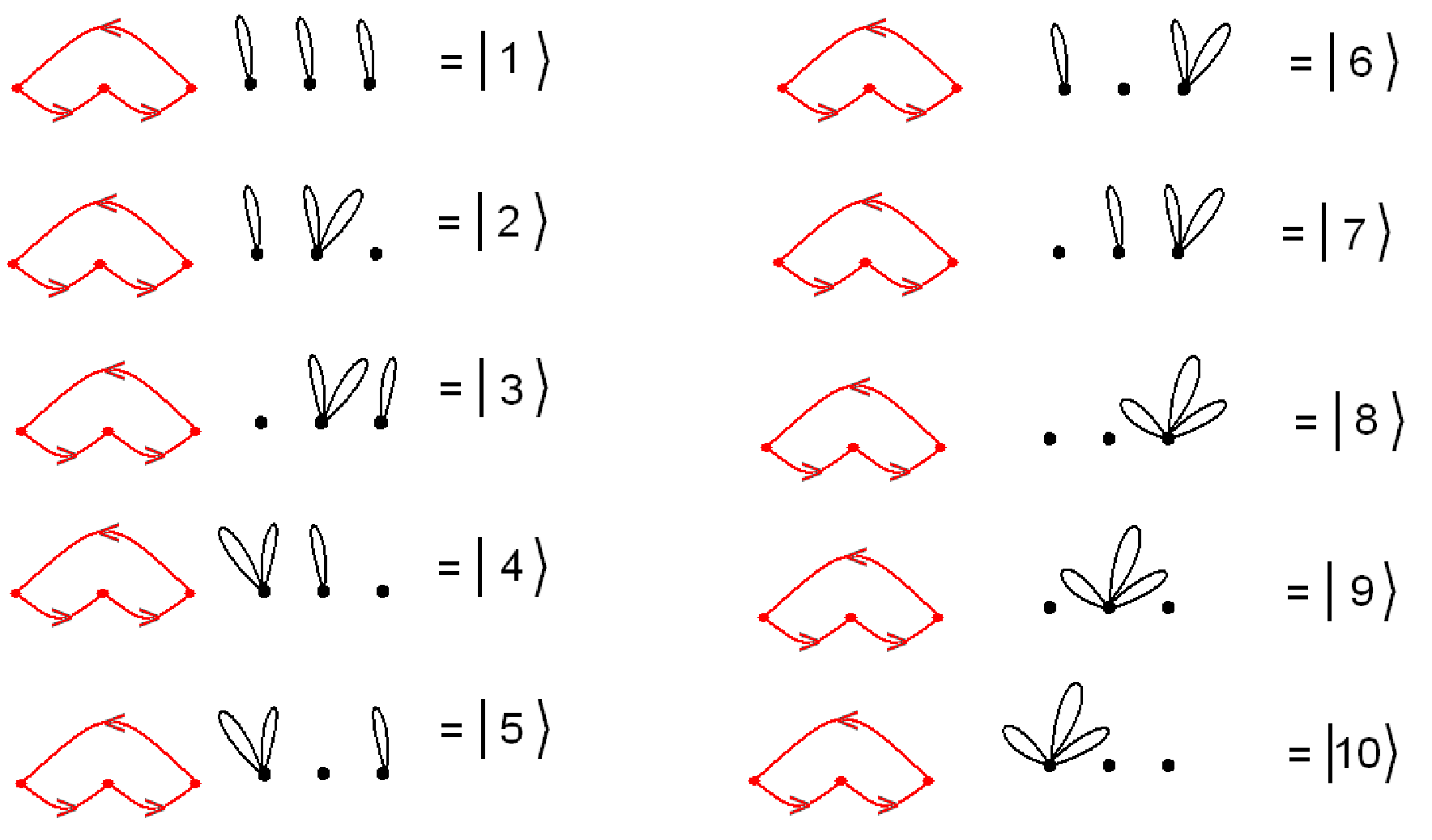
Refer to caption
Figure 3: The 10 states that appear in our first example are defined in the figure above.

Using the formulas from the previous section, there is a transition between |1⟩|1\rangle and |2⟩|2\rangle. To understand how we have labeled the dots, we must detach a loop from black node 3 of |1⟩|1\rangle and attach it to black node 2 of |2⟩|2\rangle. Denote the Gauss graph correspodning to |1⟩|1\rangle by σ1\sigma_{1} and the Gauss graph of |2⟩|2\rangle by σ2\sigma_{2}. We have n23X​(σ1)=1n_{23}^{X}(\sigma_{1})=1 (read from the red Gauss graph), n22Y​(σ1)+1=2n_{22}^{Y}(\sigma_{1})+1=2 read from |1⟩|1\rangle and n33Y​(σ1)=1n_{33}^{Y}(\sigma_{1})=1 read from |1⟩|1\rangle. Thus, in total the matrix element is

−(N+l2)​(N+l3)l2​l3​2\displaystyle-\sqrt{(N+l_{2})(N+l_{3})\over l_{2}l_{3}}\sqrt{2} (5.1)

As a second example, the matrix element for the transition between |2⟩|2\rangle and |3⟩|3\rangle is

−(N+l1)​(N+l3)l1​l3\displaystyle-\sqrt{(N+l_{1})(N+l_{3})\over l_{1}l_{3}} (5.2)

For the 10 states shown, we have the off diagonal piece of the dilatation operator given by

−(N+l1)​(N+l2)l1​l2​M12−(N+l2)​(N+l3)l2​l3​M23−(N+l1)​(N+l3)l1​l3​M13\displaystyle-\sqrt{(N+l_{1})(N+l_{2})\over l_{1}l_{2}}M_{12}-\sqrt{(N+l_{2})(N+l_{3})\over l_{2}l_{3}}M_{23}-\sqrt{(N+l_{1})(N+l_{3})\over l_{1}l_{3}}M_{13} (5.3)

where

M12=[00−20−200000000−20000−30−20000000000−20000000−3−2000000000000000−100000000−1000000000000000−300000000000−3000000]\displaystyle M_{12}=\left[\begin{array}[]{cccccccccc}0&0&-\sqrt{2}&0&-\sqrt{2}&0&0&0&0&0\cr 0&0&0&-2&0&0&0&0&-\sqrt{3}&0\cr-\sqrt{2}&0&0&0&0&0&0&0&0&0\cr 0&-2&0&0&0&0&0&0&0&-\sqrt{3}\cr-\sqrt{2}&0&0&0&0&0&0&0&0&0\cr 0&0&0&0&0&0&-1&0&0&0\cr 0&0&0&0&0&-1&0&0&0&0\cr 0&0&0&0&0&0&0&0&0&0\cr 0&-\sqrt{3}&0&0&0&0&0&0&0&0\cr 0&0&0&-\sqrt{3}&0&0&0&0&0&0\end{array}\right]
M23=[0−2000−20000−2000000000000000−20−300000−100000000−1000000−200000000000−20000−300000000−300000−300000000000000000]\displaystyle M_{23}=\left[\begin{array}[]{cccccccccc}0&-\sqrt{2}&0&0&0&-\sqrt{2}&0&0&0&0\cr-\sqrt{2}&0&0&0&0&0&0&0&0&0\cr 0&0&0&0&0&0&-2&0&-\sqrt{3}&0\cr 0&0&0&0&-1&0&0&0&0&0\cr 0&0&0&-1&0&0&0&0&0&0\cr-\sqrt{2}&0&0&0&0&0&0&0&0&0\cr 0&0&-2&0&0&0&0&-\sqrt{3}&0&0\cr 0&0&0&0&0&0&-\sqrt{3}&0&0&0\cr 0&0&-\sqrt{3}&0&0&0&0&0&0&0\cr 0&0&0&0&0&0&0&0&0&0\end{array}\right]
M13=[000−200−200000−100000000−100000000−200000000000000−2000−30000−200−300−200000000000000−3000000000000000000−300000]\displaystyle M_{13}=\left[\begin{array}[]{cccccccccc}0&0&0&-\sqrt{2}&0&0&-\sqrt{2}&0&0&0\cr 0&0&-1&0&0&0&0&0&0&0\cr 0&-1&0&0&0&0&0&0&0&0\cr-\sqrt{2}&0&0&0&0&0&0&0&0&0\cr 0&0&0&0&0&-2&0&0&0&-\sqrt{3}\cr 0&0&0&0&-2&0&0&-\sqrt{3}&0&0\cr-\sqrt{2}&0&0&0&0&0&0&0&0&0\cr 0&0&0&0&0&-\sqrt{3}&0&0&0&0\cr 0&0&0&0&0&0&0&0&0&0\cr 0&0&0&0&-\sqrt{3}&0&0&0&0&0\end{array}\right]

and we have the on diagonal piece of the dilatation operator given by

(N+l1)l1​M11+(N+l2)l2​M22+(N+l3)l3​M13\displaystyle{(N+l_{1})\over l_{1}}M_{11}+{(N+l_{2})\over l_{2}}M_{22}+{(N+l_{3})\over l_{3}}M_{13} (5.37)

where

M11=[2000000000020000000000000000000004000000000040000000000200000000000000000000000000000000000000000006]\displaystyle M_{11}=\left[\begin{array}[]{cccccccccc}2&0&0&0&0&0&0&0&0&0\cr 0&2&0&0&0&0&0&0&0&0\cr 0&0&0&0&0&0&0&0&0&0\cr 0&0&0&4&0&0&0&0&0&0\cr 0&0&0&0&4&0&0&0&0&0\cr 0&0&0&0&0&2&0&0&0&0\cr 0&0&0&0&0&0&0&0&0&0\cr 0&0&0&0&0&0&0&0&0&0\cr 0&0&0&0&0&0&0&0&0&0\cr 0&0&0&0&0&0&0&0&0&6\end{array}\right]
M22=[2000000000040000000000400000000002000000000000000000000000000000002000000000000000000000600000000000]\displaystyle M_{22}=\left[\begin{array}[]{cccccccccc}2&0&0&0&0&0&0&0&0&0\cr 0&4&0&0&0&0&0&0&0&0\cr 0&0&4&0&0&0&0&0&0&0\cr 0&0&0&2&0&0&0&0&0&0\cr 0&0&0&0&0&0&0&0&0&0\cr 0&0&0&0&0&0&0&0&0&0\cr 0&0&0&0&0&0&2&0&0&0\cr 0&0&0&0&0&0&0&0&0&0\cr 0&0&0&0&0&0&0&0&6&0\cr 0&0&0&0&0&0&0&0&0&0\end{array}\right]
M33=[2000000000000000000000200000000000000000000020000000000400000000004000000000060000000000000000000000]\displaystyle M_{33}=\left[\begin{array}[]{cccccccccc}2&0&0&0&0&0&0&0&0&0\cr 0&0&0&0&0&0&0&0&0&0\cr 0&0&2&0&0&0&0&0&0&0\cr 0&0&0&0&0&0&0&0&0&0\cr 0&0&0&0&2&0&0&0&0&0\cr 0&0&0&0&0&4&0&0&0&0\cr 0&0&0&0&0&0&4&0&0&0\cr 0&0&0&0&0&0&0&6&0&0\cr 0&0&0&0&0&0&0&0&0&0\cr 0&0&0&0&0&0&0&0&0&0\end{array}\right]

To get some insight into the structure of these matrices, note that the matrix

M=M11+M22+M33+M12+M23+M13\displaystyle M=M_{11}+M_{22}+M_{33}+M_{12}+M_{23}+M_{13} (5.71)

has eigenvalues 0,3,3,6,6,6,9,9,9,90,3,3,6,6,6,9,9,9,9. The even spacing and the degeneracy of the eigenvalues matches the weights of the symmetric representation            of S​U​(3)SU(3). This strongly suggests that, we can understand the off diagonal pieces of the dilatation operator as raising/lowering operators of some S​U​(k)SU(k) representations, with k≤gk\leq g. Recall that gg is the number of rows in our restricted Schur polynomials. This guess turns out to be correct as we now explain.

First, we need to define a bijection between the Gauss graphs that mix and the states of a particular unitary group representation. Lets start by considering a situation for which the YY Gauss graph is fixed and we have transitions between different XX Gauss graphs. We can only have transitions of closed loops between nodes ii and jj in the XX Gauss graph if ni​jY​(σ)≠0n_{ij}^{Y}(\sigma)\neq 0. Denote the number of connected components of σY\sigma^{Y} by CC. Each connected component is a set of directed line segments running between nodes. Let cc denote the number of connected components that have more than a single node. Let the number of nodes in each of these connected components be nin_{i}, i=1,…,ci=1,...,c. The irreducible representation that organizes the σX\sigma^{X} graphs is an irreducible representation of the group

SU(n1)×SU(n2)×⋯×SU(nc)\displaystyle SU(n_{1})\times SU(n_{2})\times\cdots\times SU(n_{c}) (5.72)

Focus on one of the connected components, say the jthj^{\rm th} connected component. Assume that there are a total of n~\tilde{n} closed loops attached to nodes of σX\sigma^{X} that belong to this connected component. The irreducible representation of the S​U​(nj)SU(n_{j}) factor in the above group that plays a role is labeled by a Young diagram that has a single row containing n~\tilde{n} boxes. We now want to give the map between different XX Gauss graphs and states of this representation. Number the nodes in the jthj^{\rm th} connected component from 1 up to njn_{j}. Consider an XX Gauss graph that has n11n_{11} strings attached to node 1, n22n_{22} to node 2, and so on up to nnj​njn_{n_{j}n_{j}} attached to node njn_{j}. The Gelfand-Tsetlin pattern for this state

|M⟩=[m1,njm2,nj…mnj−1,njmnj​njm1,nj−1m2,nj−1…mnj−1,nj−1………m1,2m2,2m1,1]{\footnotesize|M\rangle=\left[\begin{array}[]{ccccccc}m_{1,n_{j}}&&m_{2,n_{j}}&\dots&m_{n_{j}-1,n_{j}}&&m_{n_{j}n_{j}}\\ \vskip 6.0pt plus 2.0pt minus 2.0pt\cr&m_{1,n_{j}-1}&&m_{2,n_{j}-1}&\dots&m_{n_{j}-1,n_{j}-1}&\\ \vskip 6.0pt plus 2.0pt minus 2.0pt\cr&&\dots&\dots&\dots&&\\ \vskip 6.0pt plus 2.0pt minus 2.0pt\cr&&m_{1,2}&&m_{2,2}&&\\ \vskip 6.0pt plus 2.0pt minus 2.0pt\cr&&&m_{1,1}&&&\end{array}\right]}

has mp,q=0m_{p,q}=0 for p>1p>1 and

m1,q=∑i=1qni​i\displaystyle m_{1,q}=\sum_{i=1}^{q}n_{ii} (5.73)

This completes our discussion of how the Gauss graphs are organized, for a fixed σY\sigma^{Y}. To complete the discussion note that there is a completely parallel argument with the roles of σX\sigma^{X} and σY\sigma^{Y} switched.

As a concrete example, the Gauss graph in figure 4 corresponds to the Gelfand-Tsetlin pattern

|M⟩=[n11+n22+n3300n11+n220n11]{\footnotesize|M\rangle=\left[\begin{array}[]{ccccc}n_{11}+n_{22}+n_{33}&&0&&0\\ \vskip 6.0pt plus 2.0pt minus 2.0pt\cr&n_{11}+n_{22}&&0&\\ \vskip 6.0pt plus 2.0pt minus 2.0pt\cr&&n_{11}&&\end{array}\right]}

This map between Gelfand-Tsetlin patterns and operators labeled by Gauss graphs turns out to be useful because we know the matrix elements of the Lie algebra elements in the Gelfand-Tsetlin basis. For example, let us consider the lowering operator Ei,i+1E_{i,i+1}. This will shift ni​i→ni​i−1n_{ii}\to n_{ii}-1 and ni+1,i+1→ni+1,i+1+1n_{i+1,i+1}\to n_{i+1,i+1}+1. The net effect of these shifts in the Gelfand-Tsetlin pattern is to replace mi,k→mi,k−1m_{i,k}\to m_{i,k}-1; we will denote this pattern by Mi−M^{-}_{i}. The Gauss graph corresponding to Mi−M^{-}_{i} is obtained from the Gauss graph corresponding to MM by peeling a closed loop from node ii and reattaching it to node i+1i+1. We have already studied the matrix element of the dilatation operator that mixes these two Gauss graphs and have found

−cR​R′​cT​R′li​li+1​ni,i+1Y​(σ)​ni​iX​(σ)​(ni+1,i+1X​(σ)+1)\displaystyle-\sqrt{c_{RR^{\prime}}c_{TR^{\prime}}\over l_{i}l_{i+1}}n_{i,i+1}^{Y}(\sigma)\sqrt{n_{ii}^{X}(\sigma)(n_{i+1,i+1}^{X}(\sigma)+1)} (5.74)

where σ\sigma describes the state with Gelfand-Tsetlin pattern MM. According to [42] the matrix element for the lowering operator, written in terms of the entries of the Gelfand-Tsetlin pattern, is

⟨Mi−|Ei,i+1|M⟩=−∏k′=1l+1(mk′,l+1−mk,l+k−k′+1)​∏k′=1l−1(mk′,l−1−mk,l+k−k′)∏k′=1,k′≠kl(mk′,l+1−mk,l+k−k′+1)​(mk′,l+1−mk,l+k−k′)\displaystyle\langle M^{-}_{i}|E_{i,i+1}|M\rangle=\sqrt{-{\prod_{k^{\prime}=1}^{l+1}(m_{k^{\prime},l+1}-m_{k,l}+k-k^{\prime}+1)\prod_{k^{\prime}=1}^{l-1}(m_{k^{\prime},l-1}-m_{k,l}+k-k^{\prime})\over\prod_{k^{\prime}=1,k^{\prime}\neq k}^{l}(m_{k^{\prime},l+1}-m_{k,l}+k-k^{\prime}+1)(m_{k^{\prime},l+1}-m_{k,l}+k-k^{\prime})}} (5.75)
(5.76)
Refer to caption
Figure 4: The Gauss graph is shown in black. Closed loops can detach from a node and reattach to another node.

Plugging in the patterns for the two Gauss graphs that mix, it is straight forward to see that (5.76) evaluates to

ni​iX​(σ)​(ni+1,i+1X​(σ)+1)\displaystyle\sqrt{n_{ii}^{X}(\sigma)(n_{i+1,i+1}^{X}(\sigma)+1)} (5.77)

Comparing to (5.74) we see that the off diagonal term of the dilatation operator that we are considering is in fact

−cR​R′​cT​R′li​li+1​ni,i+1Y​(σ)​Ei,i+1\displaystyle-\sqrt{c_{RR^{\prime}}c_{TR^{\prime}}\over l_{i}l_{i+1}}n_{i,i+1}^{Y}(\sigma)E_{i,i+1} (5.78)

We will state the result for the general case, for which loops move on both the XX and YY Gauss graphs, using an example for illustration. The Gauss graph relevant for this example is show in figure 5.

Refer to caption
Figure 5: The graph on the left is σX\sigma^{X}. The graph on the right is σY\sigma^{Y}. Each node label in the above diagrams corresponds to a row number of Young diagram RR in the restricted Schur polynomial χR,(t,s,r)​μ→​ν→\chi_{R,(t,s,r)\vec{\mu}\vec{\nu}}. The Gauss graphs shown correspond to an RR with 6 long rows.

Note that σX\sigma^{X} has two connected components, one which has 2 nodes and one which has 4 nodes. Consequently the group relevant for the organization of the YYs is S​U​(2)×S​U​(4)SU(2)\times SU(4). Counting closed loops on the nodes in σY\sigma^{Y} grouped by the connected components of σX\sigma^{X} we find that the representation of S​U​(2)SU(2) we need is          while the representation of S​U​(4)SU(4) we need is                . Also, σY\sigma^{Y} has three connected components, each of which has 2 nodes. Consequently the group relevant for the organization of the YYs is S​U​(2)×S​U​(2)×S​U​(2)SU(2)\times SU(2)\times SU(2). Counting closed loops on the nodes in σX\sigma^{X} grouped by the connected components of σY\sigma^{Y} we find that the three representations for the three different S​U​(2)SU(2) groups we have are            ,            and          . Denoting the groups that appear with a superscript

G(1)×G(2)×G(3)×G(4)×G(5)=S​U​(2)×S​U​(4)×S​U​(2)×S​U​(2)×S​U​(2)\displaystyle G^{(1)}\times G^{(2)}\times G^{(3)}\times G^{(4)}\times G^{(5)}=SU(2)\times SU(4)\times SU(2)\times SU(2)\times SU(2) (5.79)

we can write the off diagonal terms in the dilatation operator as (the superscript on the Lie algebra element tells you which group it belongs to)

Doff​diagonal=−(N+l3)​(N+l4)l3​l4​(E12(2)+E21(2))−(N+l4)​(N+l5)l4​l5​(E23(2)+E32(2))\displaystyle D_{\rm off\,\,diagonal}=-\sqrt{(N+l_{3})(N+l_{4})\over l_{3}l_{4}}(E^{(2)}_{12}+E^{(2)}_{21})-\sqrt{(N+l_{4})(N+l_{5})\over l_{4}l_{5}}(E^{(2)}_{23}+E^{(2)}_{32}) (5.80)
−(N+l5)​(N+l6)l5​l6​(E34(2)+E43(2))−(N+l6)​(N+l3)l6​l3​(E14(2)+E41(2))\displaystyle-\sqrt{(N+l_{5})(N+l_{6})\over l_{5}l_{6}}(E^{(2)}_{34}+E^{(2)}_{43})-\sqrt{(N+l_{6})(N+l_{3})\over l_{6}l_{3}}(E^{(2)}_{14}+E^{(2)}_{41}) (5.81)
−2​(N+l1)​(N+l2)l1​l2​(E12(1)+E21(1))−2​(N+l3)​(N+l4)l3​l4​(E12(3)+E21(3))\displaystyle-2\sqrt{(N+l_{1})(N+l_{2})\over l_{1}l_{2}}(E^{(1)}_{12}+E^{(1)}_{21})-2\sqrt{(N+l_{3})(N+l_{4})\over l_{3}l_{4}}(E^{(3)}_{12}+E^{(3)}_{21}) (5.82)
−2​(N+l3)​(N+l4)l3​l4​(E12(4)+E21(4))−2​(N+l3)​(N+l4)l3​l4​(E12(5)+E21(5))\displaystyle-2\sqrt{(N+l_{3})(N+l_{4})\over l_{3}l_{4}}(E^{(4)}_{12}+E^{(4)}_{21})-2\sqrt{(N+l_{3})(N+l_{4})\over l_{3}l_{4}}(E^{(5)}_{12}+E^{(5)}_{21}) (5.83)

The specific representation we should use for each Lie algebra has been spelt out above.

6 Conclusions and Discussion

In this article we have evaluated certain subleading terms in the action of the dilatation operator in the S​U​(3)SU(3) sector. The operators we have studied have a classical dimension that scales as NN. Consequently, even at large NN, non-planar diagrams need to be summed and the limit we study is quite distinct from the planar limit. There is by now growing evidence that the dilatation operator in the large NN but non-planar limit can be mapped into the Hamiltonian of a set of decoupled oscillators and hence that this limit of the theory continues to enjoy integrability. In the S​U​(2)SU(2) sector, a new conservation law has been found. The corrections that we have evaluated spoil this new conservation law and consequently, these terms may be the first indiactions that the limit we consider is not integrable.

Our results clearly show that although the new terms do spoil the old conservation law, the system that emerges continues to be integrable. Indeed, the terms in the Hamiltonian that mix XX and ZZ or YY and ZZ commute with the terms that mix XX and YY, so that we simply need to change basis inside eigenspaces of fixed anomalous dimension. This change of basis has been reduced to the problem of diagonalizing certain elements in the Lie algebra of a well defined representation of a definite product of special unitary groups (the specific representation and product can be read off of the Gauss graphs as we explained in the last section). This is a solved problem in group theory.

The term in the dilatation operator that mixes XX and YY does not act on the ZZ labels. The eigenproblem in the ZZ label, after moving to the Gauss operator basis, reduces to an oscillator problem[26]. The eigenvalues of the term in the dilatation operator that mixes XX and YY sets the ground state energy of these oscillators. Note however that the BPS operators, which correspond to Gauss graphs with loops that start and end on the same node but no directed segments between nodes, are annihilated by the term in the dilatation operator that mixes XX and YY, so that these operators remain BPS even when the corrections we have computed are included.

Finally, it will be interesting to extend our analysis to the S​U​(2|3)SU(2|3) sector (and beyond) and to see if integrability persists. We leave these projects for the future.

Acknowledgements: This work is supported by the South African Research Chairs Initiative of the Department of Science and Technology and the National Research Foundation. Any opinion, findings and conclusions or recommendations expressed in this material are those of the authors and therefore the NRF and DST do not accept any liability with regard thereto. RdMK thanks Perimeter Institute for hospitality and for providing an excellent research environment. Research at Perimeter Institute is supported by the Government of Canada through Industry Canada and by the Province of Ontario through the Ministry of Economic Development & Innovation.

References

  • [1] J. M. Maldacena, “The Large NN limit of superconformal field theories and supergravity,” Adv. Theor. Math. Phys. 2 (1998) 231 [Int. J. Theor. Phys. 38 (1999) 1113] [hep-th/9711200].
  • [2] S. S. Gubser, I. R. Klebanov and A. M. Polyakov, “Gauge theory correlators from non-critical string theory,” Phys. Lett. B 428, 105 (1998) [arXiv:hep-th/9802109].
  • [3] E. Witten, “Anti-de Sitter space and holography,” Adv. Theor. Math. Phys. 2, 253 (1998) [arXiv:hep-th/9802150].
  • [4] J. A. Minahan and K. Zarembo, “The Bethe-ansatz for N = 4 super Yang-Mills,” JHEP 0303, 013 (2003) [arXiv:hep-th/0212208].
  • [5] N. Beisert, C. Kristjansen and M. Staudacher, “The dilatation operator of N = 4 super Yang-Mills theory,” Nucl. Phys. B 664, 131 (2003) [arXiv:hep-th/0303060].
  • [6] . N. Beisert et al., “Review of AdS/CFT Integrability: An Overview,” Lett. Math. Phys. 99, 3 (2012) [arXiv:1012.3982 [hep-th]].
  • [7] V. Balasubramanian, M. Berkooz, A. Naqvi and M. J. Strassler, “Giant gravitons in conformal field theory,” JHEP 0204, 034 (2002) [arXiv:hep-th/0107119].
  • [8] S. Corley, A. Jevicki and S. Ramgoolam, “Exact correlators of giant gravitons from dual N=4 SYM theory,” Adv. Theor. Math. Phys. 5 (2002) 809 [hep-th/0111222].
  • [9] R. de Mello Koch, J. Smolic and M. Smolic, “Giant Gravitons - with Strings Attached (I),” JHEP 0706 (2007) 074 [hep-th/0701066].
  • [10] R. de Mello Koch, J. Smolic and M. Smolic, “Giant Gravitons - with Strings Attached (II),” JHEP 0709 (2007) 049 [hep-th/0701067].
  • [11] Y. Kimura and S. Ramgoolam, “Branes, anti-branes and brauer algebras in gauge-gravity duality,” JHEP 0711, 078 (2007) [arXiv:0709.2158 [hep-th]].
  • [12] D. Bekker, R. de Mello Koch and M. Stephanou, “Giant Gravitons - with Strings Attached. III.,” JHEP 0802 (2008) 029 [arXiv:0710.5372 [hep-th]].
  • [13] T. W. Brown, P. J. Heslop and S. Ramgoolam, “Diagonal multi-matrix correlators and BPS operators in N=4 SYM,” arXiv:0711.0176 [hep-th].
  • [14] R. Bhattacharyya, S. Collins and R. d. M. Koch, “Exact Multi-Matrix Correlators,” JHEP 0803, 044 (2008) [arXiv:0801.2061 [hep-th]].
  • [15] T. W. Brown, P. J. Heslop and S. Ramgoolam, “Diagonal free field matrix correlators, global symmetries and giant gravitons,” arXiv:0806.1911 [hep-th].
  • [16] J. Pasukonis and S. Ramgoolam, “From counting to construction of BPS states in N=4 SYM,” arXiv:1010.1683 [hep-th].
  • [17] Y. Kimura and S. Ramgoolam, “Enhanced symmetries of gauge theory and resolving the spectrum of local operators,” Phys. Rev. D 78, 126003 (2008) [arXiv:0807.3696 [hep-th]].
  • [18] Y. Kimura, “Quarter BPS classified by Brauer algebra,” JHEP 1005, 103 (2010) [arXiv:1002.2424 [hep-th]].
  • [19] J. Pasukonis and S. Ramgoolam, “Quantum states to brane geometries via fuzzy moduli spaces of giant gravitons,” arXiv:1201.5588 [hep-th].
  • [20] Y. Kimura, “Correlation functions and representation bases in free N=4 Super Yang-Mills,” Nucl. Phys. B 865, 568 (2012) [arXiv:1206.4844 [hep-th]].
  • [21] R. Hernandez and E. Lopez, “The SU(3) spin chain sigma model and string theory,” JHEP 0404, 052 (2004) [hep-th/0403139],
    B. Stefanski, Jr. and A. A. Tseytlin, “Large spin limits of AdS/CFT and generalized Landau-Lifshitz equations,” JHEP 0405, 042 (2004) [hep-th/0404133].
  • [22] C. Kristjansen, J. Plefka, G. W. Semenoff and M. Staudacher, “A New double scaling limit of N=4 superYang-Mills theory and PP wave strings,” Nucl. Phys. B 643, 3 (2002) [hep-th/0205033].
  • [23] V. Balasubramanian, D. Berenstein, B. Feng and M. x. Huang, “D-branes in Yang-Mills theory and emergent gauge symmetry,” JHEP 0503, 006 (2005) [arXiv:hep-th/0411205].
  • [24] W. Carlson, R. d. M. Koch, H. Lin, “Nonplanar Integrability,” JHEP 1103, 105 (2011). [arXiv:1101.5404 [hep-th]].
  • [25] R. d. M. Koch, M. Dessein, D. Giataganas and C. Mathwin, “Giant Graviton Oscillators,” JHEP 1110, 009 (2011) [arXiv:1108.2761 [hep-th]].
  • [26] R. de Mello Koch, G. Kemp, S. Smith, “From Large N Nonplanar Anomalous Dimensions to Open Spring Theory,” [arXiv:1111.1058 [hep-th]].
  • [27] R. de Mello Koch and S. Ramgoolam, “A double coset ansatz for integrability in AdS/CFT,” JHEP 1206, 083 (2012) [arXiv:1204.2153 [hep-th]].
  • [28] R. d. M. Koch, G. Mashile and N. Park, “Emergent Threebrane Lattices,” Phys. Rev. D 81 (2010) 106009 [arXiv:1004.1108 [hep-th]].
  • [29] V. De Comarmond, R. de Mello Koch, K. Jefferies, “Surprisingly Simple Spectra,” JHEP 1102, 006 (2011). [arXiv:1012.3884 [hep-th]].
  • [30] R. de Mello Koch, G. Kemp, B. A. E. Mohammed and S. Smith, “Nonplanar integrability at two loops,” JHEP 1210, 144 (2012) [arXiv:1206.0813 [hep-th]].
  • [31] R. d. M. Koch, B. A. E. Mohammed and S. Smith, “Nonplanar Integrability: Beyond the SU(2) Sector,” Int. J. Mod. Phys. A 26, 4553 (2011) [arXiv:1106.2483 [hep-th]].
  • [32] R. Bhattacharyya, R. de Mello Koch and M. Stephanou, “Exact Multi-Restricted Schur Polynomial Correlators,” JHEP 0806, 101 (2008) [arXiv:0805.3025 [hep-th]].
  • [33] J. McGreevy, L. Susskind and N. Toumbas, “Invasion of the giant gravitons from Anti-de Sitter space,” JHEP 0006 (2000) 008 [hep-th/0003075].
  • [34] M. T. Grisaru, R. C. Myers and O. Tafjord, “SUSY and goliath,” JHEP 0008 (2000) 040 [hep-th/0008015].
  • [35] A. Hashimoto, S. Hirano and N. Itzhaki, “Large branes in AdS and their field theory dual,” JHEP 0008 (2000) 051 [hep-th/0008016].
  • [36] R. Giles and C. B. Thorn, “A Lattice Approach to String Theory,” Phys. Rev. D 16, 366 (1977).
  • [37] D. Berenstein, J. M. Maldacena and H. Nastase, “Strings in flat space and pp waves from N = 4 super Yang Mills,” JHEP 0204, 013 (2002) [arXiv:hep-th/0202021].
  • [38] V. Balasubramanian, M. -x. Huang, T. S. Levi and A. Naqvi, “Open strings from N=4 superYang-Mills,” JHEP 0208, 037 (2002) [hep-th/0204196].
  • [39] D. Vaman and H. L. Verlinde, “Bit strings from N=4 gauge theory,” JHEP 0311, 041 (2003) [hep-th/0209215].
  • [40] R. de Mello Koch and S. Ramgoolam, “Strings from Feynman Graph counting : without large N,” Phys. Rev. D 85, 026007 (2012) [arXiv:1110.4858 [hep-th]].
  • [41] See for example: W. Fulton and J. Harris, “Theory of Group Representations and Applications,” Springer Verlag, 1991.
  • [42] A. O. Barut and R. Raczka, “Theory of Group Representations and Applications,” 2nd ed. (PWN-Polish Scientific, Warszawa, 1986), page 280.