Time-dependent Landauer–Büttiker formula: application to transient dynamics in graphene nanoribbons
Abstract
In this work we develop a time-dependent extension of the Landauer–Büttiker approach to study transient dynamics in time-dependent quantum transport through molecular junctions. A key feature of the approach is that it provides a closed integral expression for the time-dependence of the density matrix of the molecular junction after switch-on of a bias in the leads or a perturbation in the junction, which in turn, can be evaluated without the necessity of propagating individual single-particle orbitals or Green’s functions. This allows for the study of time-dependent transport in large molecular systems coupled to wide band leads. As an application of the formalism we study the transient dynamics of zigzag and armchair graphene nanoribbons of different symmetries. We find that the transient times can exceed several hundreds of femtoseconds while displaying a long time oscillatory motion related to multiple reflections of the density wave in the nanoribbons at the ribbon–lead interface. This temporal profile has a shape that scales with the length of the ribbons and is modulated by fast oscillations described by intra-ribbon and ribbon–lead transitions. Especially in the armchair nanoribbons there exists a sequence of quasi-stationary states related to reflections at the edge state located at the ribbon–lead interface. In the case of zigzag nanoribbons there is a predominant oscillation frequency associated with virtual transitions between the edge states and the Fermi levels of the electrode. We further study the local bond currents in the nanoribbons and find that the parity of the edges strongly affects the path of the electrons in the nanoribbons. We finally study the behavior of the transients for various added potential profiles in the nanoribbons.
I Introduction
The Landauer–Büttiker (LB) formalism[1, 2] has been a real milestone in the quantum theory of charge transport. Its success is attributable to the simplicity of the LB equations, which provide a transparent and physically intuitive picture of the steady-state current, as well as to the possibility of combining the formalism with density-functional theory (DFT) for first principle calculations. [3, 4, 5, 6, 7, 8, 9] Nevertheless, due to the raising interest in the microscopic understanding of ultrafast charge transfer mechanisms, the last decade has seen heightened effort in going beyond the (steady-state) LB formalism thus accessing the transient regime. Different time-dependent (TD) approaches have been proposed to deal with different systems. Approaches based on the real-time propagation of scattering states,[10, 11, 12, 13, 14, 15] wave packets, [16, 17, 18] extended states with sharp boundaries [19, 20, 21, 22] or complex absorbing potentials, [23, 24, 25] and noninteracting Green’s functions [26, 27, 28, 29, 30, 31, 32, 33, 34, 35, 36, 37] are suited to include the electron–electron interaction in a DFT framework. Interactions can alternatively be treated using nonequilibrium diagrammatic perturbation theory and solving the Kadanoff–Baym equations for open systems.[38, 39, 40] Several nonperturbative methods have been put forward too but, at present, they are difficult to use for first-principle calculations. These include master-equation type approaches, [41, 42, 43, 44, 45, 46, 47] real-time path-integral methods,[48, 49, 50, 51] nonequilibrium renormalization group methods, [52, 53, 54, 55, 56, 57, 58] the quantum-trajectory approach,[59, 60] the TD density matrix renormalization group [61, 62, 63, 64, 65] and the nonequilibrium dynamical mean field theory. [66, 67]
In its original formulation the LB formalism treats the electrons as noninteracting. Indubitably, the neglection of the electron–electron and electron–phonon interactions is in many cases a too crude approximation. However, in the ballistic regime interaction effects play a minor role and the LB formalism is, still today, very useful to explain and fit several experimental curves. For instance the identification of the different transport mechanisms, the temperature dependence of the current, the exponential decay of the conductance as a function of the length of the junction, etc. can all be interpreted within the LB formalism.[68] The TD approaches previously mentioned have the merit of extending the quantum transport theory to the time domain. However, they all are computationally more expensive and less transparent than the LB formalism even for noninteracting electrons. Therefore, considering the widespread use of the LB formalism in both the theoretical and experimental communities, it is natural to look for a TD-LB formula which could give the current at time at the same computational cost as at the steady state.
For a single level initially isolated and then contacted to source and drain electrodes a TD-LB formula was derived by Jauho et al. in 1994.[69] The treatment of the contacts in the initial state introduces some complications which, however, were overcame about ten years later. [70] The approach of Ref. 70 was then applied to generalize the TD-LB formula to a single level with spin.[71] Nevertheless, only recently we have been able to derive a TD-LB formula for arbitrary scattering regions.[72, 73] The only restriction of this formula is that the density of states of the source and drain electrodes is smooth and wide enough that the wide-band limit approximation (WBLA) applies. In this case one can derive a TD-LB formula not only for the total current but for the full one-particle density matrix. The explicit analytic result allows for interpretion of typical transient oscillations in terms of electronic transitions within the molecular junction or between the junction and the leads, as well as the different damping times. Owing to the low computational cost one can consider very large systems and arbitrarily long propagation times.
In this work we briefly review the results of Refs. 72, 73 and generalize them to include arbitrary perturbations in the molecular junction. We further present a convenient implementation scheme to extract densities and local currents, and demonstrate the feasibility of the method in graphene nanoribbons (GNR). [74, 75, 76, 77] So far, real-time investigations of GNRs have been limited to small size[78] and weak biases.[79] As the TD-LB formalism is not limited to weak driving fields we could study the transient dynamics in the unexplored strong bias regime. In GNRs there are plenty of interesting nanoscale size effects depending on the topology of the edges. Our main findings are that for large biases (i) the time to relax to the steady state exceeds hundreds of femtoseconds; (ii) in the transient current and density of zigzag GNRs there is a predominant oscillation frequency associated with virtual transitions between the edge states and the Fermi levels of the electrodes; (iii) the currents in the armchair GNRs exhibit a sequence of quasi-stationary states whose duration increases with the length of the GNR; and (iv) the parity of the edges strongly affects the path of the electrons inside the GNR.
The paper is organized as follows. In Section II we introduce the system and present the main results of the TD-LB formalism. Here we also illustrate the implementation scheme and defer the numerical details to the Appendix. The TD results on GNRs are collected in Section III where we investigate the effects of the edge states, the quasi-stationary currents, the even–odd parity effect on the current–density profile and a perturbed GNR. Finally we draw our conclusions in Section IV.
II Theoretical background
II.1 System set-up and earlier work
We investigate quantum transport between metallic wide-band leads and a noninteracting central region. The setup is otherwise as general as possible; the number and the structure of the leads are arbitrary as is the size and the structure of the central region. The Hamiltonian is of the form
| (1) | |||||
Here is a spin index and denotes the th basis function of the th lead while and label basis states in the central region. The corresponding creation and annihilation operators for these states are denoted by and , respectively. The single-particle levels of the leads are given by while the matrices give the hoppings between the molecular and molecule–lead states. This is depicted schematically in Fig. 1.

At times the system is in thermal equilibrium at inverse temperature and chemical potential , the density matrix having the form where is the grand-canonical partition function of the connected lead–molecule system. At a sudden bias of the form
is applied to leads, where is the bias strength in lead . This potential drives the system out of equilibrium and charge carriers start to flow through the central region. To calculate the time-dependent current we use the equations of motion for the one-particle Green’s function on the Keldysh contour . This quantity is defined as the ensemble average of the contour-ordered product of particle creation and annihilation operators in the Heisenberg picture [72]
| (2) |
where the indices , can be either indices in the leads or in the central region and the variables , run on the contour. This contour has a forward and a backward branch on the real-time axis, , and also a vertical branch on the imaginary axis, describing the initial preparation of the system [39]. The matrix with matrix elements satisfies the equations of motion [80]
| (3) | |||||
| (4) |
with Kubo–Martin–Schwinger boundary conditions, i.e. the Green’s function is anti-periodic along the contour. Here is the single-particle Hamiltonian. In the basis and the matrix has the following block structure
| (5) |
where corresponds to the leads, is the coupling part, and accounts for the central region. We approximate the retarded embedding self-energy as a purely imaginary constant, according to WBLA
| (6) | |||||
In other words, the level-width functions appear as the wide-band approximation for the retarded embedding self-energy for which . Due to the coupling between the central region and the leads the matrix has nonvanishing entries everywhere
| (7) |
The equations of motion (3) and (4) for the Green’s function projected onto the central region have been solved analytically in WBLA[73] to give the time-dependent one-particle reduced density matrix (TD1RDM) as the equal-time limit :
| (8) | |||||
where is the Fermi function, and are the retarded and advanced Green’s functions, is the effective single-particle Hamiltonian, and the partial spectral functions are . The full spectral function is then simply .
We emphasize that Eq. (8) is an explicit closed formula for the equal-time or, equivalently, for the TD1RDM. All the quantities inside the integral can be calculated without the need of storing auxiliary quantities at earlier times. In other words, if we want to know the TD1RDM at time we simply need to evaluate the integral in Eq. (8). As no propagation is required we have access to nonequilibrium quantities at arbitrary times after the switch-on of the bias. This is the most important feature of Eq. (8). In fact, for large and weakly coupled junctions the transient regime can exceed several hundreds of femtoseconds and, at present, these time-scales are out-of-reach of the available TD approaches.
Similarly to the TD1RDM the time-dependent current through the interface of the th lead has an explicit closed expression which generalizes the LB formula to the time domain[73]
| (9) | |||||
where runs over all the leads. As is non-hermitian the terms in the last two rows of Eq. (9) vanish exponentially when and one recovers the steady-state LB formula. It is easy to verify that the current correctly vanishes for all at zero bias, , and for at any bias. In the remainder of this Section we present a convenient numerical procedure to evaluate Eq. (8) as well as a generalization of the same formula to include arbitrary spatially-dependent perturbations in the central region.
II.2 Expansion in the eigenbasis
We expand the result in Eq. (8) in the eigenbasis of the non-hermitian effective Hamiltonian . This object has separate left and right eigenvectors forming a mutually biorthogonal set with
| (10) |
By the biorthogonality we have , where we can choose an appropriate normalization of the diagonal elements.
We notice that in Eq. (8) in every term there is on the left and on the right. This in mind, and looking at how the matrix operates in Eq. (10) we choose to expand in the ‘left–left’ eigenbasis, i.e., we multiply the density matrix in Eq. (8) from left with a row vector and from the right by a column vector . In order to calculate a matrix element in the original basis of region we insert a complete set of left and right eigenvectors of . The resolution of identity reads
| (11) |
and hence
| (12) |
The matrix elements can easily be extracted from Eq. (8) and read
| (13) | |||||
with
| (14) |
and
| (15) |
| (16) |
| (17) |
The first row of Eq. (13) gives the steady-state value of the TD1RDM. The time dependent part is contained in the functions in the second row and in the exponential in the third row. By inspection of Eq. (13) we see that transitions between the leads and the central region are described by the terms (oscillations of frequency ), whereas transitions within the central region are described by the exponential term in the third line (oscillations of frequency ).[73] As the eigenvalues are, in general, complex we infer that electronic transitions between states in the central region are damped faster than those involving states at the Fermi energies . In the zero-temperature limit the integrals in Eq. (15-17) are given in terms of logarithms and exponential integral functions (of complex variable), which can be evaluated using an extremely accurate numerical algorithm proposed recently in the context of computer graphics,[81] see Appendix A.
II.3 Switching on of electric and magnetic fields in the central region
The TD1RDM of Eq. (8) and the TD current of Eq. (9) refer to systems driven out of equilibrium by an external bias. Here we generalize these results to include the sudden switch-on of electric and/or magnetic fields in the central region. We consider the system described in Section II.1 with central-region Hamiltonian in equilibrium and for , where is the time at which the bias is switched on. The switch-on of an electric field is useful to study, e.g., the effects of a gate voltage or to model the self-consistent voltage profile within the central region. In this case
| (18) |
where are the matrix elements of the scalar potential between two basis states of the central region. The switch-on of a magnetic field is instead useful to study, e.g., the Aharonov–Bohm effect in ring geometries or the Landau levels in planar junctions like graphene nanoribbons. In this case
| (19) |
where the sum of the Peierls phases along a closed loop yields the magnetic flux (normalized to the flux quantum ) across the loop.
Having two different Hamiltonians for the central region ( at times and at times ), we need to adjust the derivation worked out in the earlier study in Ref. 73. By definition the Matsubara Green’s function remains unchanged since it only depends on the Hamiltonian at times . On the other hand, for Green’s functions having components on the horizontal branches of the Keldysh contour, we have to use the Hamiltonian . The calculations are rather lengthy but similar to those presented in Ref. 73; we outline the main steps in Appendix B and state here only the final result for the TD1RDM
where the functions with a tilde signify that they are calculated using , except for which is to be understood as a matrix in this case (in Eq. (8) it was proportional to the identity matrix). The retarded/advanced Green’s functions in Eq. (II.3) do not have tilde since they originate from the analytic continuation of . In the limit it is easy to check that the results in Eqs. (8) and (II.3) agree.
For the case of perturbed central region we would also like to have a similar result as in Eq. (13). Since and do not necessarily commute the left/right eigenstates are not the same. For instance, in the second row of Eq. (II.3) we need to insert a complete set of left/right eigenstates of (resolution of the identity) in between the first exponential and , and so on. This leads to extra sums and overlaps between different bases. The resulting generalization of Eq. (13) is derived in Appendix B.
II.4 Physical content of the TD1RDM
From the TD1RDM in the left–left basis we can extract the matrix elements in the site basis according to Eq. (12). In the site basis the diagonal elements give the site densities (or local occupations) of the central region. The off-diagonal elements are instead related to the bond currents and the kinetic energy density.[14, 82] The site densities and the bond currents are related by the continuity equation , stating that the currents flowing in and out of site must add up to the temporal change of density in that site. It is easy to show that the bond currents are given by
| (21) |
At the steady-state () one can verify that our equations for the TD1RDM correctly imply .
III Results
We implement the framework described in the previous Section and in the Appendices to study the transient dynamics of GNRs coupled to metallic leads in the zero-temperature limit. We are especially interested to investigate the so far unexplored region of large biases, where the Dirac (low-energy) Hamiltonian is inadequate. By looking at time-dependent quantities, such as densities and bond currents, we perform a sort of spectroscopical analysis by discrete Fourier transforming the transient curves and reveal the dominant transitions responsible for the slow relaxation to a steady state.
The transport setup is shown in Fig. 2.

The leads are semi-infinite with terminal sites coupled to a GNR. The GNR is modeled by a single-orbital -electron network, parametrized by nearest neighbor hopping eV;[83] second and third nearest neighbour hoppings[83] are neglected but can be included at the same computational price. The size and the orientation [zigzag (zGNR), armchair (aGNR)] of the GNR can be chosen freely as well as the structure of the leads. The strength of the level-width functions, , depends on both the couplings to the leads and the internal properties of the leads. Even though in our framework can be any positive semidefinite matrix[84, 85] here we take it of the form
| (22) |
where when labels edge atoms contacted to lead and otherwise. In our calculations we choose eV independent of . The chemical potential is set to in order to have a charge neutral GNR in equilibrium. The system is driven out of equilibrium by a sudden symmetric bias voltage between source and drain electrodes, i.e., . The strength of the potential profile within the central region is of amplitude and can be, e.g., linear or sinusoidal as illustrated in Fig. 2, or of any other shape. To analyze the output of the numerical simulations we consider a cutting line or a bridge in the middle of the GNR and calculate the sum of all bond currents for the bonds cut by the bridge, see Fig. 2. In the following this sum of bond currents is denoted by . We measure energies in units of eV and therefore the unit of time seconds and the unit of current amperes.
III.1 Transient spectroscopy of zGNR and aGNR

Let us study the dependence of the TD current on the length of the GNR at fixed width and bias voltage. For aGNRs of width nm (this is a -aGNR where refers to the number of armchair dimer rows[86]) and a zGNRs of width nm (this is an -zGNR where is the number of zigzag rows[86]) we show in Fig. 3a-b and the Fourier transforms in Fig. 3c. The Fourier transforms are calculated from the long-time simulations shown in the inset of Fig. 3c where we subtract the steady-state value from the sample points, take the absolute value of the result and use Blackman-window filtering.[87] In both cases the bias voltage is eV and eV. By increasing the length of the ribbon the initial transient starts with a delay, since the current is measured in the center (see Fig. 2), but the steady-state value is roughly the same. The overall number of states also increases, and hence, more states close to the Fermi level are available as transport channels. Consequently smaller transition energies become dominant and the peaks in the Fourier spectra shift towards smaller frequencies. For the zGNRs we also find a high-energy peak independent of the length; this peak is responsible for the fast superimposed oscillations in the time domain. The peak appears at frequency eV and therefore corresponds to transitions between the lead Fermi energy and zero-energy states in the ribbon, i.e., the edge states. The edge states are weakly coupled to the leads and therefore these transitions are slowly damped. As a matter of fact similar high-frequency oscillations are visible in aGNRs as well, see panel a. Nevertheless, the Fourier transform does not show any high frequency peak in this case. In aGNRs we have zigzag edges at the interface and hence edge states strongly coupled to the leads. The high-frequency oscillations in aGNRs are damped faster than in zGNRs, see panel c, and are not visible in the Fourier spectrum.


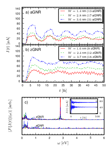
Next we vary the width of the ribbons while keeping the length and the bias voltage fixed. In Fig. 4 we show the dependency on the width for aGNRs and zGNRs of length nm. Depending on the width the ribbon is either metallic or semiconducting.[77] However, as the gap in the semiconducting case is much smaller than the applied voltage eV the conducting properties are not affected by the gap. When increasing the width of the ribbon the length of the bridge, through which the cumulative bond current is calculated, increases and so does the steady-state value of . However, the transient features remain the same as clearly illustrated in the Fourier spectrum of panel c. Thus, at difference with the results of Fig. 3c, the widening of the ribbon does not cause a shift of the low-energy peaks toward smaller energies. As expected, this is true also for the high-energy peak in zGNRs, in agreement with the fact that the energy of the edge-states is independent of the size of the ribbon.
As a third case we study the effect of increasing the bias voltage (while still keeping ). In Figs. 5a and 5c we show the results for -aGNR of length nm and width nm, and in Figs. 5b and 5c the results for -zGNR of length nm and width nm (ribbons of comparable sizes). For zGNR the frequency of the oscillations associated to the edge-state transitions increases linearly with the bias, as it should be. We also observe that for both ribbons the transient regime lasts longer the larger is the bias, and that the steady-state is attained after several hundreds of femtoseconds.
As a general remark of all the simulations shown in this subsection we can say that the absolute values of the steady-state currents are higher through zGNRs than through aGNRs (of comparable sizes). It is not easy to provide an intuitive explanation of this observation since at large biases there are very many states which contribute to the absolute value of the steady-state current. We also observe that the micro–milliampere range for the current with bias in the eV range agrees with the experimental results of Refs. 88, 89, 90, 91, 92, 93, 94, 95.
III.2 Quasi-stationary currents


In Fig. 3a we notice the formation of quasi-stationary states as we increase the length of the ribbon. The current steeply increases from zero to some value and then grows linearly before decreasing again. The growth is slower and lasts longer the longer is the ribbon. Let us investigate further the dependence of the current on the length of the ribbon. In Fig. 6 we show the transient currents through -aGNR ( nm) and -zGNR ( nm) of similar lengths with eV. For graphical purposes we normalize the current by the number of bonds in the bridge and the time by the length of the ribbon. The curves do essentially collapse on one single curve. The peculiar feature of the aGNRs is the current plateau for . The duration of the plateau corresponds to the time for an electron with velocity nm/fs to cross the ribbon. This velocity is consistent with the value of the Fermi velocity where Å is the carbon–carbon distance.[74] The physical picture is that an almost step-like, right-moving density wave reaches the bridge (positioned in the middle of the ribbon) at and the right interface at . At this time the wave is reflected backward and at time reaches the bridge thus destroying the plateau. No pronounced plateau is instead observed in zGNRs. As we shall see in the next Section the current distribution along the ribbon is strongly dependent on the orientation of the bonds. The tilted bonds in zGNRs cause multiple reflections at the edges thus preventing the formation of a current plateau. Also, more powerful reflection can be seen from the zigzag edge state (at the lead interface) in the case of aGNRs.
III.3 Even–odd parity effects in charge and current profiles


The GNRs are parametrized by integer numbers (even or symmetric and odd or asymmetric) for width and length. In this Section we study how the parity of the GNRs affects the charge and current profiles in the transient regime. We choose ribbons of equivalent lengths, approximately nm ( armchair cells and zigzag cells) and equivalent widths, approximately nm. However, we take the widths as zigzag-lines and armchair dimer-lines which, in turn, correspond to either symmetrical or asymmetrical ribbon in the longitudinal direction, see Figs. 7 and 8. A bias voltage eV is applied to the leads and is set to zero. In Figs. 7 and 8 we show snapshots of the density variation and bond-current profiles. The density variation is defined as the difference between the density at time and the ground-state density. Since the size of the ribbons is comparable to that in Sec. III.1, we choose the snapshot times to correspond to the first wavecrest, fs (on the left panels) and to the first wavetrough, fs (on the right panels). The full density and current dynamics is shown in an animation.[96]
The symmetry of the ribbon is responsible for the charge and current profiles. In the aGNR case, see Fig. 7, the top panel shows a fully symmetric -aGNR (invariant structure for mirrorings both in the transverse and longitudinal direction) and the bottom panel shows a -aGNR (invariant structure for mirroring only in the longitudinal direction). The asymmetry does not lead to dramatic differences in the charge and current distributions. In the charge profile of the symmetric aGNR certain ‘cold’ and ‘hot’ spots show up in the middle region whereas in the asymmetric aGNR the charge is more evenly distributed from the source electrode to the drain electrode. Also, in both aGNR structures the current is mostly flowing through the edges and the wavefront is flat.[96] In the zGNR case, see Fig. 8, the top panel shows an even -zGNR and the bottom panel shows an odd -zGNR. In both structures we observe diagonal charge patterns along the ribbon; in the even zGNR these patterns are symmetric whereas in the odd zGNR the patterns show asymmetric features. Certain ‘cold’ and ‘hot’ spots show up in the crossings of density wavefronts. In addition, the current is mostly flowing longitudinally through the interior of the ribbons with a much smaller contribution coming from the edges. From the animation in Ref. 96 we also see that the wavefront has a triangular shape.
The pattern of the charge–current profile is quite different at different times. On the left panels we have a perfect wave propagating along the ribbon, whereas on the right panels we see an interference pattern due to the reflected wave. In the density wave profile there are two antinodes at the electrode interfaces, at the time corresponding to the first maximum ( fs) and one antinode together with two nodes in the middle region. At the time corresponding to the first minimum ( fs) the antinodes remain at the electrode interface but additional nodes arise in the middle region.
III.4 Perturbed central region
As an illustration of the formula in Eq. (II.3) for perturbed central regions we study the transient of a -zGNR (or more accurately a ‘-by- graphene flake’). The system consists of carbon sites and an on-site potential is switched on at site concurrently with the applied bias. Let us investigate how the form of the voltage profile within the flake affects the transient dynamics. We define to be the distance of the th carbon atom from the left interface and take . For a linear potential profile we use
and for a sinusoidal potential profile
where is the length of the flake.
In Fig. 9 we show the time-dependent currents through the flake with fixed bias voltage eV and varying linear potential in panel a, and sinusoidal potential in panel b. The comparison with the previous result of non-perturbed, ‘No gate’, and perturbed, ‘ eV’, central region provides a numerical check of the correctness of Eq. (II.3).
For voltages smaller than eV the transient is not so different from the non-perturbed results. However, for stronger voltages a rather non-trivial transient behaviour is observed. Notice that the largest value eV corresponds to the physical situation of a continuous potential profile. The Fourier spectrum of the transient is shown in panel c. The much richer structure in several high-energy spectral windows is due to transitions involving levels of the perturbed central region.
The dependence of the energy and spectral weigth of the levels on is most clearly visualized by plotting the nonequilibrium spectral function
| (23) |
where the trace is over the states of the central region. The spectral function is displayed in Fig. 10. As expected the spectrum widens with increasing . The high energy peaks at eV (in the non-perturbed case: eV) shift to eV (when the perturbation is at its maximum: eV). This is consistent with the peaks occuring at around eV in Fig. 9c. With a similar analysis one can show that all other main peaks in the Fourier spectrum can be interpreted by inspecting the spectral function.
IV Conclusion
In this work we developed a time-dependent extension of the Landauer–Büttiker approach to study transient dynamics in time-dependent quantum transport through molecular junctions. We have derived a closed integral expression for the time-dependence of the density matrix of the molecular junction after switch-on of a bias voltage in the leads or a perturbation in the junction as well as for the current flowing into the leads. Both equations can be evaluated without the necessity of propagating individual single-particle orbitals or Green’s functions. We applied the approach to study the transient dynamics of zigzag and armchair graphene nanoribbons of different symmetries. We found a rich transient dynamics in which the saturation times can exceed several hundreds of femtoseconds while displaying a long time oscillatory motion related to multiple reflections of the density wave in the nanoribbons at the ribbon–lead interface. In the case of armchair nanoribbons we find pronounced quasi-steady states which can be explained by multiple reflections of the density wave passing through the ribbon with the edge states located at the ribbon–lead interfaces. We see further in the case of zigzag nanoribbons that there is a predominant oscillation frequency associated with virtual transitions between the edge states and the Fermi levels of the electrode. The transient dynamics therefore give detailed spectral information on the structure of the nanoribbons. Recently the ultrafast dynamics of individual carbon nanotubes has been measured using laser optics by four-wave mixing techniques.[97] There are therefore important experimental developments that can, in the future, give access to the direct study of transient dynamics. Such transient spectroscopy can give important detailed informations on the structure of molecular junctions out of equilibrium.
Acknowledgements.
RT wishes to thank Väisälä Foundation of The Finnish Academy of Science and Letters for financial support and CSC — the Finnish IT Center for Science — for computing resources. RvL thanks the Academy of Finland for support. EP and GS acknowledge funding by MIUR FIRB Grant No. RBFR12SW0J. GS acknowledges financial support through travel grant Psi-K2 5813 of the European Science Foundation (ESF). C. Gomes da Rocha, A.-M. Uimonen, N. Säkkinen and M. Hyrkäs are acknowledged for useful discussions.Appendix A Results in the zero-temperature limit
By taking into account the behaviour of the Fermi function in the zero-temperature limit and adjusting accordingly the integrals in Eqs. (15), (16) and (17), we get the following explicit expressions
| (24) | |||||
| (25) | |||||
| (26) |
where we defined and
| (27) |
is the principal branch complex logarithm function, the principal argument and the exponential integral function:
| (28) |
About the implementation of the complex-valued (complex variable) exponential integral there is a thorough introduction in Ref. 81. The piecewise definition of the function is due to branch cuts in the -plane.
We notice in Eqs. (24), (25) and (26) that it is possible that the structure of the single-particle Hamiltonian would together with the coupling matrices produce such an effective Hamiltonian with degenerate eigenvalues: and . In this case we consider the left/right eigenbasis of the effective Hamiltonian : Since , where and are hermitian matrices, then
| (29) | |||||
which, in turn, gives
| (30) |
Since the expectation values are real and is a positive definite matrix, we get
| (31) |
Then suppose that . This gives , and since the level-width matrices are calculated from the tunneling matrices by , we get
| (32) |
where . Having then a zero-norm vector it means that vector itself must be zero, i.e., for all . This means that is an eigenvector of with zero eigenvalue. In particular , and hence
| (33) |
Therefore the case of degenerate eigenvalues can be excluded from the derived formulae all together. This also relates to some particular systems having states that are eigenfunctions of with zero eigenvalue. In these cases, it becomes important to take into account the infinitesimal in the retarded Green’s function for these states, i.e. the Green’s function operator acting on these states has the effective form . This effectively amounts to an infinitesimal value of for these particular states in Eq. (13) which leads to sharp delta peaks in the spectral function. However, since these states are inert and do not contribute to the dynamics they only affect the static part of the density matrix. Numerically it is then more advantageous to calculate these states separately and add a cut-off in Eq. (13). We evaluate Eq. (13) only for with a small number and treat the inert states separately. The part of the density matrix corresponding to these inert states is then given by
| (34) |
where we sum over all eigenstates of that satisfy for all . Note that the existence of the inert states is a very special case caused by symmetries of the molecule and . The only case we encountered in the present study where such states exist is the case of the fully symmetric aGNR of Fig. 7. There the inert states are given by wave functions that have nodal planes exactly at the rows which are contacted to the leads.
Appendix B Results for the perturbed central region
In this Appendix we guide the reader through the derivation of Eq. (II.3). As we will often refer to results in Ref. 73 we here append the suffix “I” to every equation or section in this reference.
The results of Ref. 73 are general and remain valid in the presence of electric or magnetic fields in the central region until Sec. 3.2-I. In the Green’s function calculations the Matsubara Green’s function does not change as it depends only on the ground-state Hamiltonian . On the other hand, for Green’s functions having components on the horizontal branch of the Keldysh contour we have to use the Hamiltonian . Therefore the Eqs. (24-I) and (25-I) change according to
| (35) | |||||
| (36) |
where . All steps in Appendix C-I and D-I as well as in Sec. 3.3-I should change accordingly. In particular we stress the and in Eq. (C.9-I) are now different, that is a matrix (Appendix D-I) and that the Dyson-like equation [Eq. (D.1-I)] relating the non-perturbed and perturbed Green’s functions now reads
| (37) |
With these considerations and following the same steps as in Ref. 73 we arrive at the result shown in Eq. (II.3).
Next, by expanding in the left eigenbasis of we find
| (38) |
with the introduced functions
where eigenvalues and refer to the complex eigenvalues of and , respectively. In the limit this result can also be checked to reduce to the earlier result in Eqs. (13), (15), (16) and (17). In the limit of uncontacted system Eq. (38) describes the dynamics of an isolated (perturbed) system, in which case the same result could be derived directly from the equations of motion of the one-particle density matrix.
In the zero-temperature limit, the integrals in Eq. (B) can be calculated analytically also in this case. The integrals now only have more constants and the final results can not be simplified as much as earlier. The explicit forms can be found below
| (40) | |||||
| (41) | |||||
| (42) | |||||
where and is as in Eq. (27). Also these results can be checked to reduce to the earlier results in Eqs. (24), (25) and (26) when and ().
References
- [1] R. Landauer, IBM J. Res. Dev. 1, 223 (1957).
- [2] M. Büttiker, Phys. Rev. Lett. 57, 1761 (1986).
- [3] N. D. Lang, Phys. Rev. B 52, 5335 (1995).
- [4] N. D. Lang and P. Avouris, Phys. Rev. Lett. 81, 3515 (1998).
- [5] J. Taylor, H. Guo, and J. Wang, Phys. Rev. B 63, 121104 (2001).
- [6] J. Taylor, H. Guo, and J. Wang. Phys. Rev. B 63, 245407 (2001).
- [7] M. Brandbyge, J. L. Mozos, P. Ordejon, J. Taylor, and K. Stokbro, Phys. Rev. B 65, 165401 (2002).
- [8] G. Stefanucci and C.-O. Almbladh, Europhys. Lett. 67, 14 (2004).
- [9] F. Evers, F. Weigend, and M. Koentopp, Phys. Rev. B 69, 235411 (2004).
- [10] S. Kurth, G. Stefanucci, C.-O. Almbladh, A. Rubio, and E. K. U. Gross, Phys. Rev. B 72, 035308 (2005).
- [11] X. Qian, J. Li, X. Lin, and S. Yip, Phys. Rev. B 73, 035408 (2006).
- [12] G. Stefanucci, E. Perfetto, and M. Cini, Phys. Rev. B 78, 075425 (2008).
- [13] Z. Zhou and S.-I. Chu, Europhys. Lett. 88, 17008 (2009).
- [14] G. Stefanucci, E. Perfetto, and M. Cini, Phys. Rev. B 81, 115446 (2010).
- [15] B. Gaury et al., Phys. Rep. 534, 1 (2014)
- [16] P. Bokes, F. Corsetti, and R. W. Godby, Phys. Rev. Lett. 101, 046402 (2008).
- [17] A. Chaves, G. A. Farias, F. M. Peeters, and B. Szafran, Phys. Rev. B 80, 125331 (2009).
- [18] P. Bokes, Phys. Rev. A 83, 032104 (2011).
- [19] N. Bushong, N. Sai, and M. D. Ventra, Nano Lett 5, 2569 (2005).
- [20] C.-L. Cheng, J. S. Evans, and T. V. Voorhis, Phys. Rev. B 74, 155112 (2006).
- [21] N. Sai, N. Bushong, R. Hatcher, and M. DiVentra, Phys. Rev. B 75, 115410 (2007).
- [22] H. Eshuis and T. van Voorhis, Chem. Phys. Phys. Chem. 11, 10293 (2009).
- [23] R. Baer, T. Seideman, S. Ilani, and D. Neuhauser, J. Chem. Phys. 120, 3387 (2004).
- [24] K. Varga, Phys. Rev. B 83, 195130 (2011).
- [25] L. Zhang, J. Chen, and J. Wang, Phys. Rev. B 87, 205401 (2013).
- [26] J. Maciejko, J. Wang, and H. Guo, Phys. Rev. B 74, 085324 (2006).
- [27] X.-Q. Li and Y. J. Yan, Phys. Rev. B 75, 075114 (2007).
- [28] V. Moldoveanu, V. Gudmundsson, and A. Manolescu, Phys. Rev. B 76, 085330 (2007).
- [29] A. Prociuk and B. D. Dunietz, Phys. Rev. B 78, 165112 (2008).
- [30] A. Croy and U. Saalmann, Phys. Rev. B 80, 245311 (2009).
- [31] X. Zheng et al., J. Chem. Phys. 133, 114101 (2010).
- [32] Y. Xing, B. Wang, and J. Wang, Phys. Rev. B 82, 205112 (2010).
- [33] H. Xie et al., J. Chem Phys. 137, 044113 (2012).
- [34] L. Zhang, Y. Xing, and J. Wang, Phys. Rev. B 86, 155438 (2012).
- [35] A. Pertsova, M. Stamenova, and S. Sanvito, J. Phys.: Cond. Matt. 25, 105501 (2013).
- [36] Y. Zhang, S. Chen, and G. H. Chen, Phys. Rev. B 87, 085110 (2013).
- [37] E. McEniry et al., J. Phys.: Condens. Matter 19, 196201 (2007).
- [38] P. Myöhänen, A. Stan, G. Stefanucci, and R. van Leeuwen, Europhys. Lett. 84, 67001 (2008).
- [39] P. Myöhänen, A. Stan, G. Stefanucci, and R. van Leeuwen, Phys. Rev. B 80, 115107 (2009).
- [40] M. Puig von Friesen, C. Verdozzi, and C.-O. Almbladh, Phys. Rev. B 82, 155108 (2010).
- [41] J. N. Pedersen and A. Wacker, Phys. Rev. B 72, 195330 (2005).
- [42] S. Welack, M. Schreiber, and U. Kleinekathöfer, J. Chem. Phys. 124, 044712 (2006).
- [43] H. Wang and M. Thoss, J. Chem. Phys. 131, 024114 (2009).
- [44] V. Moldoveanu, V. Gudmundsson, and A. Manolescu, New J. Phys. 11, 073019 (2009).
- [45] P. Zedler, G. Schaller, G. Kiesslich, C. Emary, and T. Brandes, Phys. Rev. B 80, 045309 (2009).
- [46] J. N. Pedersen and A. Wacker, Physica E 42, 595 (2010).
- [47] S. Wang, X. Zheng, J. Jin, and Y. J. Yan, Phys. Rev. B 88, 035129 (2013).
- [48] S. Weiss, J. Eckel, M. Thorwart, and R. Egger, Phys. Rev. B 77, 195316 (2008).
- [49] M. Schiro and M. Fabrizio, Phys. Rev. B 79, 153302 (2009).
- [50] D. Segal, A. J. Millis, and D. R. Reichman, Phys. Rev. B 82, 205323 (2010).
- [51] G. Cohen and E. Rabani, Phys. Rev. B 84, 075150 (2011).
- [52] F. B. Anders and A. Schiller, Phys. Rev. Lett. 95, 196801 (2005).
- [53] F. B. Anders and A. Schiller, Phys. Rev. B 74, 245113 (2006).
- [54] M. Pletyukhov, D. Schuricht, and H. Schoeller, Phys. Rev. Lett. 104, 106801 (2010).
- [55] P. Wang and S. Kehrein, Phys. Rev. B 82, 125124 (2010).
- [56] S. Andergassen, M. Pletyukhov, D. Schuricht, H. Schoeller, and L. Borda, Phys. Rev. B 83, 205103 (2011).
- [57] D. M. Kennes, S. G. Jakobs, C. Karrasch, and V. Meden, Phys. Rev. B 85, 085113 (2012).
- [58] E. Eidelstein, A. Schiller, F. Guttge, and F. B. Anders, Phys. Rev. B 85, 075118 (2012).
- [59] X. Oriols, Phys. Rev. Lett. 98, 066803 (2007).
- [60] G. Albareda, J. Sune, and X. Oriols, Phys. Rev. B 79, 075315 (2009).
- [61] G. Vidal, Phys. Rev. Lett. 93, 040502 (2004).
- [62] P. Schmitteckert, Phys. Rev. B 70, 121302 (2004).
- [63] S. R. White and A. E. Feiguin, Phys. Rev. Lett. 93, 076401 (2004).
- [64] A. Branschädel, G. Schneider, and P. Schmitteckert, Ann. Phys. 522, 657 (2010).
- [65] U. Schollwöck, Ann. Phys. 326, 96 (2011).
- [66] P. Werner, T. Oka, and A. J. Millis, Phys. Rev. B 79, 035320 (2009).
- [67] P. Werner, T. Oka, M. Eckstein, and A. J. Millis, Phys. Rev. B 81, 035108 (2010).
- [68] See for instance, J. C. Cuevas and E. Scheer, Molecular Electronics: An Introduction to Theory and Experiments, World Scientific, 2010.
- [69] A.-P. Jauho, N. S. Wingreen, and Y. Meir, Phys. Rev. B 50, 5528 (1994).
- [70] G. Stefanucci and C.-O. Almbladh, Phys. Rev. B 69, 195318 (2004).
- [71] E. Perfetto, G. Stefanucci, and M. Cini, Phys. Rev. B 78, 155301 (2008).
- [72] G. Stefanucci and R. van Leeuwen, Nonequilibrium Many-Body Theory of Quantum systems: A Modern Introduction, Cambridge Univerisity Press, 2013.
- [73] R. Tuovinen, R. van Leeuwen, E. Perfetto, and G. Stefanucci, J. Phys.: Conf. Ser. 427, 012014 (2013).
- [74] A. H. C. Neto, F. Guinea, N. M. R. Peres, K. S. Novoselov, and A. K. Geim, Rev. Mod. Phys. 81, 109 (2009).
- [75] M. I. Katsnelson, Graphene: Carbon in Two Dimensions, Cambridge Univerisity Press, 2012.
- [76] A. Onipko, Phys. Rev. B 78, 245412 (2008).
- [77] K. Wakabayashi, K. Sasaki, T. Nakanishi, and T. Enoki, Sci. Tech. Adv. Mater. 11, 054504 (2010).
- [78] H. Xie et al., Phys. Status Solidi B 250, 2481 (2013).
- [79] E. Perfetto, G. Stefanucci, and M. Cini, Phys. Rev. B 82, 035446 (2010).
- [80] L. P. Kadanoff and G. Baym, Quantum Statistical Mechanics, Benjamin, 1962.
- [81] V. Pegoraro and P. Slusallek, Journal of Graphics, GPU and Game Tools, 15, 183 (2011).
- [82] I. V. Tokatly, Phys. Rev. B 83, 035127 (2011).
- [83] Y. Hancock, A. Uppstu, K. Saloriutta, A. Harju, and M. J. Puska, Phys. Rev. B 81, 245402 (2010).
- [84] H. Schomerus, Phys. Rev. B 76, 045433 (2007).
- [85] Y. M. Blanter and I. Martin, Phys. Rev. B 76, 155433 (2007).
- [86] K. Wakabayashi, Y. Takane, M. Yamamoto, and M. Sigrist, New J. Phys. 11, 095016 (2009).
- [87] R. B. Blackman and J. W. Tukey, Particular Pairs of Windows: In The Measurement of Power Spectra, From the Point of View of Communications Engineering (pp. 98–99), Dover, 1959.
- [88] X. Wang et al., Phys. Rev. Lett. 100, 206803 (2008).
- [89] M.-W. Lin et al., Nanotechnology 22, 265201 (2011).
- [90] X. Li, X. Wang, L. Zhang, S. Lee, and H. Dai, Science 319, 1229 (2008).
- [91] Y. Lu, C. A. Merchant, M. Drndić, and A. T. C. Johnson, Nano Letters 11, 5184 (2011).
- [92] Q. Yan et al., Nano Letters 7, 1469 (2007).
- [93] G. Liang et a.l, IEEE Trans. Electron Dev. 54, 677 (2007).
- [94] I. Meric et al., Nature Nanotech. 3, 654 (2008).
- [95] Z. Li, H. Qian, J. Wu, B.-L. Gu, and W. Duan, Phys. Rev. Lett. 100, 206802 (2008).
- [96] See Supplemental Material at http://link.aps.org/supplemental/10.1103/PhysRevB.89.085131 for the animations corresponding to Figs. 7 and 8.
- [97] P. Myllyperkiö et al., ACS Nano 4, 6780 (2010).