The generalized pseudospectral approach to the bound states of Hulthén and Yukawa potentials
Abstract
The generalized pseudospectral method is employed to calculate the bound states of Hulthén and Yukawa potentials in quantum mechanics, with special emphases on higher excited states and stronger couplings. Accurate energy eigenvalues, expectation values and radial probability densities are obtained through a nonuniform and optimal spatial discretization of the radial Schrödinger equation. Results accurate up to thirteen to fourteen significant figures are reported for all the 55 eigenstates of both these potentials with 10 for arbitrary values of the screening parameters covering a wide range of interaction. Furthermore, excited states as high as up to have been computed with good accuracy for both these potentials. Excellent agreement with the available literature data has been observed in all cases. The states of Yukawa potential has been considerably improved over all other existing results currently available, while the same for Hulthén potential are reported here for the first time. Excepting the and states of Yukawa potential, the present method surpasses in accuracy all other existing results in the stronger coupling region for all other states of both these systems. This offers a simple and efficient scheme for the accurate calculation of these and other screened Coulomb potentials.
I Introduction
The screened Coulomb potentials,
| (1) |
of which Hulthén and Yukawa potentials are two simple representatives, have been of considerable interest in the context of many physical systems and a considerable amount of work has been devoted to study their numerous features over the years. Z is identified as the atomic number when these are used in the context of atomic systems, while the screening parameter has different significance in different branches. The Hulthén potential [1] is one of the most important short-range potentials and has been used in the nuclear and particle physics [2-5], atomic physics [6-7], solid-state physics [8-9], chemical physics [10], etc. This is also a special case of the Eckart potential. The Yukawa potential [11], on the other hand, has found applications in approximating the effects of screening of nuclear charges by plasmas (commonly termed as the Debye-Hückel potential), shielding effect in the atoms and also in the solid-state physics (as the Thomas-Fermi potential), etc.
These two potentials have several similarities; e.g., they are both Coulomb-like for small and decay monotonically exponentially to zero for large . Another distinctive feature of these potentials (in contrast to the Coulomb potentials) is the presence of limited number of bound states characterized by the presence of the screening parameters; i.e., bound states exist only for certain values of the screening parameter below a threshold limit (e. g., for the Yukawa potential, this value has been accurately estimated as 1.19061227 0.00000004 [12] in atomic units). The former has the additional special property that it offers exact analytical solutions for states only, not for the higher partial waves [13]. Many formally attractive and efficient formalisms have been proposed for accurate determination of the eigenvalues, eigenfunctions as well as for the values of the critical screening parameters differing in complexity, accuracy and efficiency. The most notable of these are the variational calculations employing a multitude of basis functions [14-18,12], combined Padé approximation and perturbation theory [19-21], shifted 1/N approximation along with many of its variants [22-27], dynamical-group approach [28], supersymmetric quantum mechanics [29], numerical calculations [30-31,18] and other works [32-33].
In the past few years, the generalized pseudospectral (GPS) method has been proved to be a very powerful and efficient tool to deal with the static and dynamic processes of many-electron atomic/molecular systems characterized by the Coulomb singularities (see, for example, [34-37] and the references therein). Recently it has also been successfully applied to the power-law and logarithmic potentials [38], as well as the spiked harmonic oscillator with stronger singularity [39]. One of the objectives of this article is to extend and explore the regions of validity of this formalism to a different class of singularities, namely the screened Coulomb potentials thus covering a broader range of physical systems. In an attempt to assess the performance and its applicability to such systems, we have computed all the 55 eigenstates (110) of the Hulthén and Yukawa potentials and compared them with the available literature data wherever possible with an aim to study the spectra of these systems systematically. It may be noted that although many accurate results are available for these potentials in the weaker coupling region and for the lower states, there is a lack of good quality results in the stronger region and for the higher states. In this work, we pay special attention to both of these issues. Screening parameters of arbitrary field strengths (covering both weak and strong limits of interaction) have been considered for given values of and quantum numbers. To this end, accurate calculations have been performed on the eigenvalues, expectation values and radial probability densities of these two systems. As a further stringent test of the method, we calculate some very high excited states (up to ) of these two systems which have been examined never before. As will be evident in a later section, this method is indeed capable of producing excellent quality results comparable in accuracy to the other existing literature data for both these systems and in many cases (especially in the stronger regions of coupling), indeed offers the best results. The article is organized as follows: Section II presents an outline of the theory and the method of calculation. Section III gives a discussion on the results while section IV makes some concluding remarks.
II The GPS method for the solution of the Hulthén and Yukawa potentials
In this section, we present an overview of the GPS formalism within the nonrelativistic framework for solving the radial Schrödinger equation (SE) of a single-particle Hamiltonian containing a Hulthén or Yukawa term in the potential. Only the essential steps are given and the relevant details may be found elsewhere ([34-39] and the references therein). Unless otherwise mentioned, atomic units are employed throughout this article.
The radial SE can be written in the following form,
| (2) |
where
| (3) |
or
| (4) |
where and denote the respective screening parameters whereas and signify the usual radial and angular momentum quantum numbers respectively. Use of a scaling transformation, gives the following well-known relation,
| (5) |
Thus it suffices to study only the case and this fact has been used in this work. The usual finite difference or finite element discretization schemes often require a large number of grid points to achieve good accuracy and convergence, often because of their uniform nature. The GPS formalism, in contrast, can give nonuniform and optimal spatial discretization with a significantly smaller number of grid points allowing a denser mesh at smaller and a coarser mesh at larger while maintaining similar accuracies in both regions. In addition, this is also computationally orders of magnitude faster.
The first step is to approximate a function defined in the interval by the N-th order polynomial such that,
| (6) |
and this ensures that the approximation is exact at the collocation points , i.e.,
| (7) |
Here, we have used the Legendre pseudospectral method having , , where are obtained from the roots of the first derivative of the Legendre polynomial with respect to , i.e.,
| (8) |
The in Eq. (6) are called the cardinal functions and given by,
| (9) |
These have the unique property, . Now the semi-infinite domain can be mapped onto the finite domain by the transformation . The following algebraic nonlinear mapping,
| (10) |
may be used, where L and are termed as the mapping parameters. Now, introduction of the following relation,
| (11) |
followed by a symmetrization procedure leads to the transformed Hamiltonian as below,
| (12) |
where is given by,
| (13) |
The advantage is clear; this leads to a symmetric matrix eigenvalue problem which can be readily solved to give accurate eigenvalues and eigenfunctions by using some standard available routines. Note that for the particular transformation used here and finally one obtains the following set of coupled equations,
| (14) |
where
| (15) |
and the symmetrized second derivatives of the cardinal function, are given by,
| (16) |
with
| (17) | |||||
A large number of tests have been performed to check the accuracy and reliability of the method so as to produce “stable” results with respect to the variation of the mapping parameters. In this way, a consistent set of parameter sets were chosen. For the problems at hand and seemed appropriate for all the states considered in this work while values were varied as required (see later). The results are reported only up to the precision that maintained stability. It may be noted that all our results are truncated rather than rounded-off.
III Results and Discussion
Let us first examine the convergence of the calculated energy eigenvalues. As an illustration, consider the following two cases of states of the Hulthén potential which offer exact analytical results: (a) the ground state with (high screening) and (b) (moderately high state) with (intermediate screening). Variation of the eigenvalues was monitored with respect to the radial distance keeping the other two parameters and N fixed at 25 and 200 respectively. It was seen that or 300 a. u., was not suitable for either of these situations (although these may be sufficient for weaker screenings) and with a. u., a reasonable convergence can be achieved. However, a better convergence in both these cases requires at least a. u. And after that, the calculated results are stable with respect to . As expected, for even higher states one would require a larger ; e. g., the state with same requires a. u. However, the results are apparently less sensitive with respect to , the total number of grid points; only 200 points is sufficient for all the calculations reported in this work. This is in sharp contrast with the finite difference (FD) or finite element (FE) methods where one usually requires a substantially larger number of radial grid points to achieve good convergence for such singular systems. This is more so, if one uses a uniform discretization scheme. The present method does not suffer from such an uncomfortable feature, for it offers equally accurate eigenfunctions both at small and the large distances with significantly smaller grid points. For a given screening parameter, within a particular , the required increases with increasing . For a given state, larger screening parameter requires larger . For example, the states of Hulthén potential reach convergence with a. u., for ; but needed a.u. Similar considerations hold equally good for the Yukawa potential.
| State | Energy | Energy | ||||
|---|---|---|---|---|---|---|
| This work | Reference | This work | Reference | |||
| (2.0) | 0.002 | 0.49900050000000 | 0.499000511 1 Ref. [23].,0.4990005* | 1.97 | 0.00011249999999 | 0.0001125* |
| (0.5) | 0.025 | 0.11281249999999 | 0.112812499996022 2 Ref. [31].,0.1128125* | 0.492 | 0.00003200000000 | 0.000032* |
| (0.222) | 0.002 | 0.05456005555555 | 0.0545600611 1 Ref. [23]., 0.054560055* | 0.21 | 0.00016805555555 | 0.000168055* |
| (0.008) | 0.001 | 0.0014851250000 | 0.001485125* | 0.005 | 0.0002531250000 | 0.000253125* |
| (0.007) | 0.001 | 0.0012662288062 | 0.0012662288062* | 0.005 | 0.0001332288062 | 0.0001332288062* |
Now let us consider the states of Hulthén potential which offer exact analytical results [1,13] given by,
| (18) |
with . Table I presents the calculated eigenvalues for some representative states with at selected values of . For each of these states, two screening parameters are chosen; weak in the left- and strong in the right-hand side. The critical screening parameters () for S states, given by the simple relation, [18], are presented in the parentheses in column 1 along with the states. The exact eigenvalues calculated from the above are given with an asterisk at the end. As noted, in the weaker region as well as for lower states, other theoretical results are available, while no reference theoretical results could be found for higher states as well as for the stronger coupling cases. Because of their exactly solvable nature, some of these states (especially the lower ones like and ) have received extra attention from various workers employing a variety of methods and we have quoted a few of them. Some of these include the Lie algebraic method [40], Padé approximation [19], path integral formulation [41], shifted 1/N expansion [23], dynamical group theoretical consideration [28], generalized variational calculation [16] as well as the accurate numerical calculation [31], etc. First, we note that the calculated values completely coincide with the exact analytical results for all these states encompassing the whole range of interaction nicely. This amply demonstrates the accuracy, reliability and potential of the methodology. For , shifted 1/N expansion results [23] are available in the weak coupling region and the present results are considerably superior to these values in all cases. For , accurate numerical eigenvalues [31] are available for . Their results are significantly better than the . For states, results of [31] are comparable to ours, but for the states, current values are superior to [31]. Quite accurate results have been reported [16] for states that improved the previous results in the literature significantly by employing trial wave functions which were linear combinations of independent functions. Results of [16] are better than ours in the weak-coupling region, but in the stronger limit, our results are noticeably better than [16]. It may be mentioned that we have enlarged the coupling region from all other previous works and it is clear that the current results are so far the most accurate values in regions closest to the critical limit. For states with , no other theoretical results are available in the literature so far and we hope that these results may be helpful in future studies. It may be mentioned that the energies of states are slightly less accurate than the other lower state energies.
| State | Energy | State | Energy | ||||
|---|---|---|---|---|---|---|---|
| This work | Literature | This work | Literature | ||||
| 0.005 | 0.12251041674479 | 0.01 | 0.02640009031711 | 0.0264022 2 Ref. [33]. | |||
| 0.35 | 0.00379309814702 | 0.0037930981470211 1 Ref. [16]. | 0.08 | 0.00135376897143 | |||
| 0.36 | 0.00220960766773 | 0.005 | 0.01756564260992 | ||||
| 0.005 | 0.05308159769106 | 0.05 | 0.00178354579471 | 0.0017835457947111 1 Ref. [16]. | |||
| 0.15 | 0.00446630878535 | 0.0044663087853511 1 Ref. [16]. | 0.005 | 0.01755731319688 | |||
| 0.18 | 0.00047689388317 | 0.05 | 0.00101588159045 | 0.0010158815904511 1 Ref. [16]. | |||
| 0.005 | 0.05307743154020 | 0.005 | 0.01148061249746 | ||||
| 0.15 | 0.00139659246573 | 0.0013965924657311 1 Ref. [16]. | 0.025 | 0.00372009346428 | 0.0037200934642811 1 Ref. [16]. | ||
| (0.098) | 0.075 | 0.00383453307692 | 0.0038345330769211 1 Ref. [16]. | 0.005 | 0.01147020315553 | ||
| 0.09 | 0.00099103405815 | 0.025 | 0.00346543458707 | 0.0034654345870711 1 Ref. [16]. | |||


Next in table II we present energies of the representative non-zero angular momentum states of the Hulthén potential with . As already mentioned, these states do not offer exact analytical results and a large number of attempts have been made over the years, e.g., the variational as well as numerical integration [18], strong-coupling expansion [42], supersymmetric quantum mechanics [29], parameter-free wave function approach based on the local properties such as the cusp conditions [31], etc., in addition to some of the methods which also dealt with the case such as [16,19,24,28,31]. Other works include [7,43,44] and the best results are quoted here for comparison. The s in these cases cannot be obtained by a simple form and an approximate analytical expression was put forth by [42],
| (19) |
which offered results rather in good agreement with the numerically determined values [18]. These values from [18] are given in parentheses. Majority of the previous works have dealt with the weak coupling regions. We have chosen values for all the states quite wide; from weak to strong. A uniform accuracy is maintained for all these states in the whole region of interaction, unlike some other previous calculations which encountered difficulties in the stronger limits (e.g., the break- down of the shifted 1/N expansion method for ground state with [23]). In the weaker limit, our computed eigenvalues are superior to all other results except the accurate variational calculations [16]. However in this work, we have gone beyond the interaction region considered in [16] or in any other previous calculation so far for some of these states (, , , ) and no results could be found for these states for direct comparison. Now Fig. 1 depicts the variation of energy eigenvalues with screening parameter for all the states belonging to (left) and (right) respectively. For small values of the principal quantum number, there is a resemblance of the energy orderings as those with the Coulomb potentials, but with an increase in , significant deviations from the Coulomb potential ordering and complex level crossings observed in the vicinity of zero energy. This is more pronounced in the latter case (, mixing heavily with , , and at around ) and for higher , there is a gradual increase in the probability of energy ordering becoming more complex, which make their accurate calculations quite difficult. We also notice that for a particular value of , the separation between states with different values of increases with . Additionally now in table III we give the calculated eigenvalues for all the states belonging to and 10 at 0.01 values respectively. While states with relatively higher values have been studied for the Yukawa potential (see later), no results have been reported so far for such higher states of the Hulthén potential. For the sake of completeness, here also the values are quoted from [18].
| State | Energy | State | Energy | ||
|---|---|---|---|---|---|
| 0.02 | 0.0009868327076 | 0.01 | 0.0012427752748 | ||
| 0.02 | 0.0009349530511 | 0.01 | 0.0012282621767 | ||
| 0.02 | 0.0008556949061 | 0.01 | 0.0012063302045 | ||
| 0.02 | 0.0007470911124 | 0.01 | 0.0011767752007 | ||
| 0.02 | 0.0006060126055 | 0.01 | 0.0011393080783 | ||
| 0.02 | 0.0004274312523 | 0.01 | 0.0010935375130 | ||
| 0.02 | 0.0002027526409 | 0.01 | 0.0010389439316 | ||
| 0.01 | 0.0009748402143 | ||||
| 0.01 | 0.0009003110142 |
| State | Energy | Energy | ||||
|---|---|---|---|---|---|---|
| This work | Literature | This work | Literature | |||
| (1.1906) | 0.01 | 0.40705803061340 | 0.4070580306134011 1 Ref. [31].,22 2 Ref. [16].,33 3 Ref. [21]. | 1.19 | 0.00000010303196 | 0.0000001030319633 3 Ref. [21]. |
| (0.2202) | 0.01 | 0.11524522409056 | 0.1152452240905622 2 Ref. [16].,33 3 Ref. [21]. | 0.22 | 0.00002869724498 | 0.0000286922 2 Ref. [16].,0.00002633 3 Ref. [21]. |
| (0.1127) | 0.01 | 0.04615310482916 | 0.0461644 4 Ref. [30].,0.0461555 5 Ref. [33]. | 0.11 | 0.00022634084060 | |
| (0.0913) | 0.01 | 0.04606145416065 | 0.0460644 4 Ref. [30].,55 5 Ref. [33]. | 0.09 | 0.00031291350263 | |
| (0.0581) | 0.01 | 0.02222779248980 | 0.0222277924898022 2 Ref. [16]. | 0.055 | 0.00049188376726 | |
| (0.0498) | 0.005 | 0.02646809608410 | 0.0264744 4 Ref. [30].,0.0264555 5 Ref. [33]. | 0.045 | 0.00148735974333 | 0.0014655 5 Ref. [33]. |
| (0.0354) | 0.01 | 0.01142540016608 | 0.0114254001660822 2 Ref. [16]. | 0.035 | 0.00006899773341 | |
| (0.0313) | 0.01 | 0.01126616478845 | 0.0112661647884522 2 Ref. [16]. | 0.031 | 0.00009981963916 | |
| (0.0264) | 0.005 | 0.00944274896286 | 0.0094427489628622 2 Ref. [16]. | 0.025 | 0.00019933872619 | 0.0002044 4 Ref. [30]. |
| (0.0238) | 0.005 | 0.00940059908613 | 0.0094005990861322 2 Ref. [16]. | 0.022 | 0.00042240106329 | |
| (0.0215) | 0.005 | 0.00934767158207 | 0.0093476715820722 2 Ref. [16]. | 0.021 | 0.00016299459024 | |


Now we turn our focus on to the Yukawa potentials. Table IV presents the calculated eigenvalues of some representative states with at selected values of the screening parameter (weak and strong screenings in the left and right respectively). Lower states have been examined by many methods; e.g., Rayleigh-Schrödinger perturbation expansion [21], variational methods [6,15,16], Padé approximations [20], shifted 1/N expansions [22,25], numerical calculations through direct integration of the SE [30] or by the Ritz method [31], etc. Other works include [12,33]. However, excepting a few of these (like [21] or [16]), majority of them produce good-quality results in the weaker regions of interaction, and are often fraught with difficulties in the stronger regions (e.g., the shifted 1/N expansion [22] runs into trouble for near the critical values). The best available literature data are given for comparison. The numerically determined critical screening parameters ()s for these states are quoted from [30]. First of all, very good agreement is observed for all these states with the best available literature data. Once again a wide range of interaction region has been considered and the converged results are uniformly accurate for all of these states for arbitrary values of . We note that, accurate numerical results [31] have been reported for the , and states in the weaker coupling region. Our results are as accurate as those of [31], while those for and states are superior to [31]. As in the case of Hulthén potential, results of [16] are more accurate than ours for smaller , but we have obtained better results in the stronger regions (e. g., the states with respectively). Very accurate energies were reported in [21] for states having both small and large s. Results of [21] are better than ours for the first two states, but for the state present results deviate considerably from [21] in the stronger region (e. g., ) and we believe these are the better results. Some of these states have not been calculated by any method other than those of [30,33], and the GPS results improve those values dramatically. Thus to our knowledge, these appear to be the most accurate results for these states (except ) in the regions closest to the critical domain. In Fig. 2 we graphically show the dependence of the energy orderings of all the (left) and (right) states of the Yukawa potential on the screening parameter in the vicinity of E=0. Essentially similar qualitative features are observed as in Fig. 1 for the Hulthén potential, viz. (a) gradually more complex level crossings as increases and (b) the energy splitting between the states with different values of for a given value of increases with an increase in the screening parameter. Table V gives all the eigenstates for and 10 at selected values of respectively. As and increase, calculation of these states become progressively difficult, and only two attempts have been made so far to study the states, viz., the direct numerical integration of SE [30] as well as the shifted 1/N expansion [22]. The former results are more accurate than the latter and these are quoted. While their works [30] estimated these states fairly accurately and still by far the most reliable values reported in the literature, clearly the present results are much more improved in accuracy. The values in these cases are taken from [30]. No attempts are known for any of the states with and here we have given them for the first time which may constitute a useful reference for future studies. Also in this table are included the results for some of the representative states with up to 17 and no comparisons could be made because of the lack of literature data.
| State | Energy | State | Energy | ||||
|---|---|---|---|---|---|---|---|
| This work | Literature [30] | This work | Literature | ||||
| (0.016) | 0.01 | 0.0005858247612 | 0.000585 | 0.005 | 0.0015083559307 | ||
| (0.015) | 0.01 | 0.0005665076261 | 0.000565 | 0.005 | 0.0015009235029 | ||
| (0.014) | 0.01 | 0.0005276644203 | 0.00053 | 0.005 | 0.0014860116240 | ||
| (0.013) | 0.01 | 0.0004688490636 | 0.00047 | 0.005 | 0.0014635239275 | ||
| (0.012) | 0.01 | 0.0003893108558 | 0.00039 | 0.005 | 0.0014333097805 | ||
| (0.011) | 0.01 | 0.0002878564558 | 0.00029 | 0.005 | 0.0013951561294 | ||
| (0.0107) | 0.005 | 0.0022606077422 | 0.00226 | 0.005 | 0.0013487749860 | ||
| (0.0100) | 0.005 | 0.0021997976659 | 0.00220 | 0.005 | 0.0012937846259 | ||
| (0.0094) | 0.005 | 0.0021291265596 | 0.00213 | 0.005 | 0.0012296811835 | ||
| 0.005 | 0.0011557947569 | 0.002 | 0.002455067336 | ||||
| 0.002 | 0.001849081136 | 0.002 | 0.001392026936 | ||||
| 0.001 | 0.001122878263 | 0.001 | 0.000919120394 | ||||
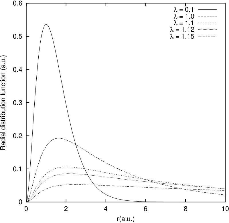
As a further test of the convergence of eigenfunctions, the calculated density moments and are given in table VI for a few states at selected values of the screening parameters of both Hulthén (left) and Yukawa (right) potentials. The best available numerical results [31] are quoted in the parentheses wherever available, and for all these instances, we have obtained superior results than the previous reported values in literature. Additionally, the left portion of Fig. 3 shows the variation of radial probability distribution functions for ground states of the Yukawa potential with respect to . Five values of are considered, viz., 0.1 (low screening), 1.0 and 1.1 (moderate screening), 1.12 and 1.15 (high screening). It is seen that with an increase in , the density distribution oozes out to larger values of and the peak values are reduced. The right portion of Fig. 3 depicts the density distributions for , and states of the Yukawa potential with . As expected it spreads out to larger as increases and the requisite number of nodes are present. Analogous features are also observed for the Hulthén potential. At this stage, a few comments should be made. It has been pointed out [16] that the eigenvalues of Coulomb, Hulthén and the Yukawa potentials follow the relation,
| (20) |
and this has been verified to be satisfied for all the states considered in this work. Finally, we mention here that the GPS method employed here possesses the simplicity of FD or FE methods and at the same time retain the attractive features of the basis-set variational methods, such as high accuracy and fast convergence. It is also known that it guarantees an “exponential” (also called infinite-order) convergence for a given problem with smooth (infinitely differentiable) solutions (which is usually the case) as long as the orthogonal functions employed belong to a common singular Sturm-Liouville class. Furthermore, a pseudospectral method with N+1 or N+2 grid points is usually equivalent in accuracy to the corresponding basis-set expansion method with N basis functions (for a detailed account of these and other features of GPS method, see [34-39, 44,45] and the references therein).
| State | ||||||
|---|---|---|---|---|---|---|
| 0.1 | 0.998748957029 | 1.502506265664 | 0.5 | 0.867533084978 | 1.806554897095 | |
| (0.867533084) | (1.806554897) | |||||
| 0.1 | 0.244953137615 | 6.113636363636 | 0.1 | 0.227996338490 | 6.529952268703 | |
| (0.2279963389) | (6.52995228) | |||||
| 0.001 | 0.111109986106 | 13.50011475165 | 0.001 | 0.111104429011 | 13.50068154934 | |
| 0.001 | 0.00387414697 | 386.4792127 | 0.001 | 0.00375246427 | 396.3082404 | |
| 0.001 | 0.00342393411 | 437.0760155 | 0.001 | 0.00329034570 | 450.9901509 |
IV conclusion
A detailed study has been made on the accurate eigenvalues, density moments and radial densities of Hulthén and Yukawa potentials by employing the GPS formalism. The methodology is simple, efficient, accurate and reliable. Special attention has been paid to the higher excited states as well the stronger screening effects. All the 55 states belonging to have been computed with good accuracy and the results are compared wherever possible. In the weak coupling regions, our results are comparable to all other accurate literature results available (except [21] and [16]), while in the strong coupling region, present results are noticeably superior to all other existing results for all states of both these systems excepting the and states of Yukawa potential. The states of Yukawa potentials are significantly improved from the best available data available so far, while the same for Hulthén potential are reported here for the first time. In view of the simplicity and accuracy offered by this method for both these physical systems studied in this work, it is hoped that this may be equally successful and useful for other singular potentials in various branches of quantum mechanics.

Acknowledgements.
I gratefully acknowledge the warm hospitality provided by the University of New Brunswick, Fredericton, NB, Canada. I am greatly thankful to the anonymous referee for numerous valuable comments.References
- [1] L. Hulthén, Ark. Mat. Astron. Fys. 28A, 5 (1942); 29B, 1 (1942).
- [2] L. Hulthén and M. Sugawara, in Encyclopedia of Physics, edited by S. Flügge (Springer, Berlin, 1957), Vol. 39.
- [3] B. Durand and L. Durand, Phys. Rev. D 23, 1092 (1981).
- [4] M. Mishra, S. N. Jena and T. N. Tiwari, Pramana 32, 1 (1989).
- [5] W. van Dijk, Phys. Rev. C 40, 1437 (1989).
- [6] C. S. Lam and Y. P. Varshni, Phys. Rev. A 4, 1875 (1971).
- [7] R. Dutt and U. Mukherji, Phys. Lett. A 90A, 395 (1982).
- [8] C. S. Lam and Y. P. Varshni, Phys. Rev. A 6, 1391 (1972).
- [9] C. S. Lam and Y. P. Varshni, Phys. Status Solidi B 89, 103 (1978).
- [10] J. A. Olson and D. A. Micha, J. Chem. Phys. 68, 4352 (1978).
- [11] H. Yukawa, Proc. Phys. Math. Soc. Jpn. 17, 48 (1935).
- [12] O. A. Gomes, H. Chacham and J. R. Mohallem, Phys. Rev. A 50, 228 (1994).
- [13] S. Flügge, Practical Quantum Mechanics (Springer, Berlin, 1974).
- [14] K. M. Roussel and R. F. O’Connell, Phys. Rev. A 9, 52 (1974)
- [15] R. L. Greene and C. Aldrich, Phys. Rev. A 14, 2363 (1976).
- [16] C. Stubbins, Phys. Rev. A 48, 220 (1993).
- [17] V. Fessatidis, J. D. Mancini, Q. Haider, Y. Zhou and L. Greco, Phys. Lett. A 242, 74 (1998).
- [18] Y. P. Varshni, Phys. Rev. A 41, 4682 (1990).
- [19] C. S. Lai and W. C. Lin, Phys. Lett. A 78, 335 (1980).
- [20] C. S. Lai, Phys. Rev. A 23, 455 (1981).
- [21] E. R. Vrscay, Phys. Rev. A 33, 1433 (1986).
- [22] T. Imbo, A. Pagnamenta and U. Sukhatme, Phys. Lett. A 105A, 183 (1984).
- [23] A. Z. Tang and F. T. Chan, Phys. Rev. A 35, 911 (1987).
- [24] B. Roy and R. Roychoudhury, J. Phys. A 20, 3051 (1987).
- [25] H. Christiansen, L. N. Epele, H. Fanchiotti and C. A. Garcia Canal, Phys. Rev. A 40, 1760 (1989).
- [26] G. Moreno and A. Zepeda, J. Phys. B 17, 21 (1984)
- [27] A. Chatterjee, J. Phys. A 18, 1193 (1985); ibid., 18, 2403 (1985).
- [28] P. Matthys and H. De Meyer, Phys. Rev. A 38, 1168 (1988).
- [29] B. Gönül, O. Özer, Y. Cançelic and M. Koçak, Phys. Lett. A 275, 238 (2000).
- [30] F. J. Rogers, H. C. Graboske, Jr., and J. Harwood, Phys. Rev. A 1, 1577 (1970).
- [31] M. A. Núñez, Phys. Rev. A 47, 3620 (1993).
- [32] R. L. Hall, J. Phys. A 25, 1373 (1992).
- [33] S. H. Patil, J. Phys. A 34, 3153 (2001).
- [34] X. M. Tong and S. I. Chu, Phys. Rev. A 55, 3406 (1997); ibid. 64, 013417 (2001).
- [35] D. Telnov and S. I. Chu, Phys. Rev. A 59, 2864 (1999).
- [36] A. K. Roy and S. I. Chu, Phys. Rev. A 65, 043402 (2002); ibid. 65, 052508 (2002).
- [37] A. K. Roy and S. I. Chu, J. Phys. B 35, 2075 (2002).
- [38] A. K. Roy, J. Phys. G 30, 269 (2004).
- [39] A. K. Roy, Phys. Lett. A 321, 231 (2004).
- [40] B. I. Dunlap and L. Armstrong, Phys. Rev. A 6, 1370 (1972).
- [41] J. M. Cai, P. Y. Cai and A. Inomata, Phys. Rev. A 34, 4621 (1986).
- [42] S. H. Patil, J. Phys. A 17, 575 (1984).
- [43] V. S. Popov and V. M. Weinberg, Phys. Lett. A 107, 371 (1985).
- [44] C. H. Lai, J. Math. Phys. 28, 1801 (1987).
- [45] D. Gottlieb, M. Yousuff and S. A. Orszag, in Spectral Methods for Partial Differential Equations, Eds. R. G. Voigt, D. Gottlieb and M. Y. Hussaini (SIAM, Philadelphia, 1984).
- [46] C. Canuto, M. Y. Hussaini, A. Quarteroni and T. A. Zang, Spectral Methods in Fluid Dynamics (Springer, Berlin, 1988).