Schwarzschild scalar wigs: spectral analysis and late time behavior

Juan Barranco Affiliation: Departamento de Física, División de Ciencias e Ingenierías, Campus León, Universidad de Guanajuato, León 37150, México Argelia Bernal Affiliation: Área Académica de Matemáticas y Física, Universidad Autónoma del Estado de Hidalgo, Carretera Pachuca-Tulancingo Km. 4.5, C.P. 42184, Pachuca, Hidalgo, México Juan Carlos Degollado Affiliation: Departamento de Física da Universidade de Aveiro and I3N, Campus de Santiago, 3810-183 Aveiro, Portugal Alberto Diez-Tejedor Affiliation: Departamento de Física, División de Ciencias e Ingenierías, Campus León, Universidad de Guanajuato, León 37150, México Affiliation: SCIPP and Department of Physics, University of California, Santa Cruz, CA, 95064, USA Miguel Megevand Affiliation: Department of Physics and Astronomy, Louisiana State University, Baton Rouge, LA 70803-4001, USA Affiliation: Instituto de Ciencias Nucleares, Universidad Nacional Autónoma de México, Circuito Exterior C.U., A.P. 70-543, México D.F. 04510, México Miguel Alcubierre Affiliation: Instituto de Ciencias Nucleares, Universidad Nacional Autónoma de México, Circuito Exterior C.U., A.P. 70-543, México D.F. 04510, México Darío Núñez Affiliation: Instituto de Ciencias Nucleares, Universidad Nacional Autónoma de México, Circuito Exterior C.U., A.P. 70-543, México D.F. 04510, México Olivier Sarbach Affiliation: Instituto de Física y Matemáticas, Universidad Michoacana de San Nicolás de Hidalgo, Edificio C-3, Ciudad Universitaria, 58040 Morelia, Michoacán, México

August 24, 2026

Abstract

Using the Green’s function representation technique, the late time behavior of localized scalar field distributions on Schwarzschild spacetimes is studied. Assuming arbitrary initial data we perform a spectral analysis, computing the amplitude of each excited quasi-bound mode without the necessity of performing dynamical evolutions. The resulting superposition of modes is compared with a traditional numerical evolution with excellent agreement; therefore, we have an efficient way to determine final black hole wigs. The astrophysical relevance of the quasi-bound modes is discussed in the context of scalar field dark matter models and the axiverse.

pacs

95.30.Sf 04.70.-s 98.62.Mw 95.35.+d

I Introduction

Scalar fields show up in many areas of physics. In the standard model of particle physics they are necessary to give particles their observed mass. At the effective level, the charged pions mediating the strong nuclear interaction are described by a scalar field. Another example is provided by the axion, introduced in order to resolve the strong CP problem in quantum chromodynamics. Generically, a plethora of scalar fields emerge in the axiverse from super-string and higher dimensional theories [1, 2, 3, 4, 5, 6, 7, 8]. In a cosmological context, a scalar field could guide an early phase of exponential expansion, also represent the dark energy, and possibly even the dark matter in the present Universe [9, 10, 11, 12, 13, 14, 15, 16, 17, 18, 19, 20, 21, 22, 23, 24, 25, 26, 27, 28].

On the other hand, black holes are a natural consequence of general relativity. They appeared for the first time as a purely mathematical result, but they were later recognized as real astrophysical objects. Presently, we believe black holes represent the final fate of sufficiently massive stars, and supermassive black holes probably reside at the center of most galaxies [29].

Since both scalar fields and black holes seem to inhabit our Universe, a natural question arises: How do scalar fields and black holes interact with each other? Static, spherically symmetric, asymptotically flat black holes with a non-trivial scalar field distribution cannot exist in nature [30, 31]; however, these results do not rule out extremely long lived transient phenomena [32, 33].

The massive Klein-Gordon equation on a black hole background has been studied extensively. For a Schwarzschild black hole Ternov et al. [34] found the existence of quasi-bound modes (also called quasi-stationary modes or quasi-resonances), describing scalar field configurations surrounding the black hole for some period of time; see also Refs. [35, 36] for later work on these states. Similar modes were found on a Kerr black hole background [34, 37, 38]. In the rotating case, there is a specific range of parameters for which these modes are exponentially growing in time, implying that a massive scalar field on a rotating Kerr black hole is unstable. See Refs. [39, 40, 41, 42] for rigorous results on this instability, and [43, 44, 45] for recent numerical studies. Based on Leaver’s continuous fraction method [46], Konoplya and Zhidenko [47] computed the quasi-normal frequencies of a massive scalar field on a Schwarzschild spacetime background, and mentioned conditions under which quasi-bound states could arise. For a generalization to the Kerr-Newman case, see Ref. [48]. Finally, we mention that Dolan and collaborators [49, 50] generalized the computation of quasi-bound modes to different types of fields, vectorial or fermionic.

Motivated by the possibility of describing the dark matter in the galactic halo by the coherent excitation of an ultra-light scalar field [9, 10, 11, 12, 13, 14, 15, 16, 17, 18, 19, 20, 21, 22, 23, 24, 25, 26, 27, 28], including the supermasive black hole [51, 52, 53, 54], in previous work we analyzed the time scale for the quasi-bound states on a supermassive, nonrotating black hole background [32, 33]; see [55] for a recent generalization to the Dirac field. In particular, we showed in Ref. [33] that these states can actually survive for cosmological times, as long as the product of the black hole and the scalar field mass is sufficiently small. Furthermore, we provided strong evidence in Ref. [33] that these quasi-bound modes are generic. This conclusion was reached by numerically evolving arbitrary initial data and Fourier-transforming the solution with respect to time. The spectrum revealed a clear excitation of the quasi-bound frequencies.

In this paper we use the Green’s function representation technique [56] to determine the late time behavior of localized scalar field distributions on a Schwarzschild background. Within this technique, the Green’s function of the problem is decomposed into three contributions, corresponding to different contours in the complex frequency plane. The contribution we are focusing on in this work is the one arising from the residua of the poles of the Green’s function, which describe the excitations of the quasi-bound states. This allows us to predict, given arbitrary initial data for the scalar field on a spacelike hypersurface, the amplitude of each quasi-bound state in the solution by computing a simple, one-dimensional integral. Furthermore, we show by comparison with results obtained from numerical evolutions that for large times (within the time scales of our simulations) the behavior of the solution is well approximated by the corresponding superposition of quasi-bound sates; therefore, the remaining two contributions to the Green’s function become negligible for those times. Note that this situation is different than the case of a massless scalar field propagating on a Schwarzschild background, where the oscillating part of the solution, described by a superposition of quasi-normal modes, is soon taken over by the slower, polynomial tail decay. This difference resides in the fact that the quasi-bound modes have a decay rate which is much smaller than the quasi-normal modes, so that they dominate the solution for much larger time.

At this point we would like to stress that our definition of “large” or “late” times in this article is the following: we consider time scales which are very large compared to the Schwarzschild radius of the black hole, but which are within the lifetime of the quasi-bound states. In particular, we do not claim that for $t\to\infty$ the solution is described by a simple superposition of quasi-bound states since in this limit the contribution from the tail part is expected to play an important role. However, for the physical scenario we are interested in, it is enough to consider large times which, according to our definition, could be larger than the age of the universe as we explained above.

Our results provide the basis for a generalization to the case of a rotating black hole. Several lines of work have been developed in the context of scalar and other fields on Kerr background; there are those which consider unstable modes in the vicinity of the Kerr black hole [57, 58], and even possible radiation emission due to such instabilities [59, 60]. The continuation of our work, however, will focus on a somewhat different direction, namely the scalar field in the Kerr background in connection with dark matter halos.

The remaining part of this work is organized as follows. In Sec. II we briefly review the Green’s function method and the corresponding decomposition of the solution in three different contributions. Next, in Sec. III we discuss the case of a potential formed by a delta and a step function, as a toy model for which the modes can be represented analytically. In particular, we determine the quasi-bound frequencies in the limit for which the height of the step is very small compared to the amplitude of the delta barrier and show that they are located very close to the resonant band, resulting in very small decay rates. Then, we compute the excitations of each quasi-bound state, compare the resulting superposition to the results obtained from a numerical evolution, and find a very good agreement at late times.

In Sec. IV we apply the Green’s function technique to the case of a massive scalar field on a Schwarzschild background. Here the modes and quasi-bound frequencies are computed semianalytically via a matching algorithm from which the excitation amplitudes can be determined. In Sec. V we compare the semianalytic results with those obtained from numerical evolutions of the Cauchy problem, and as in the case of the toy model, for late times we find an excellent agreement between the two approaches. Then, in Sec. VI we use our semianalytic solution to extract some physical properties of the quasi-bound states that might be relevant in the astrophysical context, and finally in Sec. VII we present our conclusions.

We also include two appendixes. In the first one we generalize the Green’s function technique to time foliations different than the one arising from standard Schwarzschild coordinates. In the second appendix we provide some estimates on the location of the quasi-bound frequencies for the toy model example and the time after which the solution can be described by a superposition of the corresponding modes.

II Green’s function representation and spectroscopy

In this section we briefly review the Green’s function representation technique and the corresponding decomposition of the integral kernel. We will concentrate on the solution of $1+1$ dimensional wave problems with time-independent, non-negative potentials $V(x)$ ; see the original paper by Leaver [56] and the review articles [61, 62, 63] for further details. Therefore, we consider the Cauchy problem

	$\frac{\partial^{2}\phi}{\partial t^{2}}-\frac{\partial^{2}\phi}{\partial x^{2}}+V(x)\phi=0,$	(1a)
with $t>0$ , $x\in\mathbb{R}$ , and initial data
	$\phi(0,x)=\phi_{0}(x),\quad\frac{\partial\phi}{\partial t}(0,x)=\pi_{0}(x).$	(1b)

We assume $\phi_{0}$ and $\pi_{0}$ to be smooth and compactly supported. In this paper we will be interested only in the late time behavior.

The solution of the problem in Eqs. (1) can be represented in terms of an integral kernel $k(t,x,y)$ ,

\phi(t,x)=\int\limits_{-\infty}^{\infty}\frac{\partial k}{\partial t}(t,x,y)\phi_{0}(y)dy+\int\limits_{-\infty}^{\infty}k(t,x,y)\pi_{0}(y)dy,

(2)

where $k(t,x,y)$ can formally be written as

k(t,x,y)=\frac{1}{2\pi i}\int\limits_{s=\eta-i\infty}^{\eta+i\infty}e^{st}G(s,x,y)ds,\qquad\eta>0,

(3)

with $G(s,x,y)=G(s,y,x)$ the Green’s function,

G(s,x,y):=\frac{1}{W(s)}\left\{\begin{array}[]{ll}f_{-}(s,y)f_{+}(s,x),&y\leq x\\ f_{-}(s,x)f_{+}(s,y),&y>x\end{array}\right\}.

(4)

Here $f_{+}(s,x)$ and $f_{-}(s,x)$ are two nontrivial solutions of the mode equation $s^{2}f-f^{\prime\prime}+V(x)f=0$ with exponential decay at $x\to+\infty$ and $x\to-\infty$ , respectively, when $\mbox{Re}(s)>0$ , and the prime denotes the derivative with respect to the variable $x$ . $W(s)$ is their Wronski determinant defined as

W(s):=\det\left(\begin{array}[]{ll}f_{+}(s,x)&f_{-}(s,x)\\ f_{+}^{\prime}(s,x)&f_{-}^{\prime}(s,x)\end{array}\right).

(5)

Note that $W(s)$ does not depend on $x$ , and by definition, it is zero if and only if the two solutions $f_{+}(s,\cdot)$ and $f_{-}(s,\cdot)$ are proportional to each other.

A priori, the Green’s function is a well-defined, analytic function on the right complex plane $\mbox{Re}(s)>0$ . However, it is interesting to consider its analytic continuation to the left complex plane $\mbox{Re}(s)<0$ since this offers the possibility to “close” the integration contour in Eq. (3), as illustrated in Fig. 1. As a consequence, the kernel typically splits into a sum of three different contributions,

k(t,x,y)=k_{\textrm{modes}}(t,x,y)+k_{\textrm{tail}}(t,x,y)+k_{\textrm{hfa}}(t,x,y).

(6)

Here, $k_{\textrm{modes}}$ is a sum over the residua of the poles of the analytic continuation of the Green’s function, and each term in the sum is proportional to $e^{s_{n}t}$ . These terms describe the resonances; they oscillate with frequency $\omega_{n}=\mbox{Im}(s_{n})$ and their amplitude decays exponentially in time since $\mbox{Re}(s_{n})<0$ . Next, $k_{\textrm{tail}}$ is the contribution that comes from the integration around the branch cuts, and it is usually associated with the tail decay, giving rise to a polynomial decay of the form $t^{-p}$ for some $p>0$ . Finally, $k_{\textrm{hfa}}$ is the contribution from the high-frequency arc (see the curve $\mu_{R}$ in Fig. 1). This contribution is highly dependent on the initial data; however, it vanishes for large enough $t$ .

Refer to caption — Figure 1: The branch cut (broken lines) for the analytic function $\kappa(s)$ defined in Eq. (23) and the deformation of the curve $\gamma$ which allows to close the integration contour.

Of course, the structure of the analytic continuation of the Green’s function (including the location of the poles and the branch cuts) depends on the potential $V(x)$ and the problem at hand. In the next section, we analyze this structure for the case of a simple toy model, and we show that all the poles are located close to the resonant band $i(-\mu,\mu)$ and give rise to quasi-bound states. Based on this analysis we expect the structure of the analytic continuation to be very similar in the case of a massive scalar field propagating on a Schwarzschild black hole.

In this work we are mainly interested in the contribution from the poles, that is, $k_{\textrm{modes}}$ , since in our context this is the part corresponding to the quasi-bound states. The poles, $s_{n}$ , of the Green’s function are determined by the zeros of the Wronskian $W(s)$ ; notice that at such zeros the functions $f_{+}(s_{n},\cdot)$ and $f_{-}(s_{n},\cdot)$ are linearly dependent. Assuming that $W(s)$ has only simple zeros at $s=s_{n}$ , that is, $W(s)=\alpha_{n}(s-s_{n})+{\cal O}(s-s_{n})^{2}$ , with

\alpha_{n}:=\left.\frac{d}{ds}W(s)\right|_{s=s_{n}}\neq 0,

(7)

the mode contribution to the solution from the $n$ ’th mode $s_{n}$ is given by

	$\phi_{\textrm{modes},n}(t,x)=A_{n}e^{s_{n}t}f_{+}(s_{n},x),$			(8a)
with amplitude

	$\displaystyle A_{n}$	$\displaystyle:=$	$\displaystyle\left.\left[\frac{d}{ds}W(s)\right]^{-1}\right\|_{s=s_{n}}$	(8b)
		$\displaystyle\times$	$\displaystyle\int\limits_{-\infty}^{\infty}f_{-}(s_{n},y)[s_{n}\phi_{0}(y)+\pi_{0}(y)]dy.$	(8b)

When the potential $V(x)$ in Eq. (1a) is real, the poles come in complex conjugate pairs, $s_{-n}=s_{n}^{*}$ , and since $W(s)$ and $f_{\pm}(s,x)$ are analytic functions in $s$ , the sum $\phi_{\textrm{modes},n}(t,x)+\phi_{\textrm{modes},-n}(t,x)$ is real.

For a generalization of these expressions to more general foliations by spacelike hypersurfaces, see Appendix A.

III A toy model example

Before applying the Green’s function technique just described to the scalar field problem on a Schwarzschild black hole we consider the following simple toy model potential [33]:

V(x)=A\delta(x)+\mu^{2}\theta(x-a),

(9)

consisting of a delta-barrier with positive amplitude $A$ at $x=0$ and a step function at $x=a>0$ , where $V(x)$ jumps from zero to its asymptotic value $\mu^{2}$ . (Do not confuse the amplitude $A$ in the potential, with the amplitudes $A_{n}$ of the quasi-bound modes.) As it turns out, this model captures all the rough qualitative features of the scalar field problem.

In order to construct the Green’s function for the potential in Eq. (9), we consider first the region $x<0$ , where $V(x)=0$ , such that


$\displaystyle f_{-}(s,x)$	$\displaystyle=$	$\displaystyle e^{sx},$	(10a)
$\displaystyle f_{+}(s,x)$	$\displaystyle=$	$\displaystyle a_{+}(s)e^{-sx}+b_{+}(s)e^{sx}.$	(10b)

Notice that $f_{-}(s,\cdot)$ decays exponentially at $x\to-\infty$ when $\mbox{Re}(s)>0$ , as required. The coefficients $a_{+}(s)$ and $b_{+}(s)$ are unknown to this point and will be determined by the matching conditions. In the region $0<x<a$ , the two solutions have the form


$\displaystyle f_{-}(s,x)$	$\displaystyle=$	$\displaystyle c_{-}(s)e^{-sx}+d_{-}(s)e^{sx},$	(11a)
$\displaystyle f_{+}(s,x)$	$\displaystyle=$	$\displaystyle c_{+}(s)e^{-sx}+d_{+}(s)e^{sx},$	(11b)

with coefficients $c_{\pm}(s)$ , $d_{\pm}(s)$ . Finally, in the region $x>a$ , where $V(x)=\mu^{2}$ , we have


$\displaystyle f_{-}(s,x)$	$\displaystyle=$	$\displaystyle a_{-}(s)e^{-\kappa(s)x}+b_{-}(s)e^{\kappa(s)x},$	(12a)
$\displaystyle f_{+}(s,x)$	$\displaystyle=$	$\displaystyle e^{-\kappa(s)x},$	(12b)

with coefficients $a_{-}(s)$ and $b_{-}(s)$ ; and where we have defined $\kappa(s):=\sqrt{s^{2}+\mu^{2}}$ with the choice for the sign such that $\mbox{Re}(\kappa(s))>0$ for $\mbox{Re}(s)>0$ , such that $f_{+}(s,\cdot)$ has the required asymptotic behavior at $x\to+\infty$ .

Because of the delta-barrier, the matching conditions at $x=0$ consist of the continuity of the functions $f_{\pm}(s,\cdot)$ , and the jump condition $f_{\pm}^{\prime}(s,0^{+})-f_{\pm}^{\prime}(s,0^{-})=Af_{\pm}(s,0)$ for their derivatives. At $x=a$ , both $f_{\pm}(s,\cdot)$ and $f_{\pm}^{\prime}(s,\cdot)$ need to be continuous. These matching conditions yield the following values for the coefficients $c_{\pm}(s)$ and $d_{\pm}(s)$ :


$\displaystyle c_{-}(s)$	$\displaystyle=$	$\displaystyle-\frac{A}{2s},$	(13a)
$\displaystyle d_{-}(s)$	$\displaystyle=$	$\displaystyle 1+\frac{A}{2s},$	(13b)
$\displaystyle c_{+}(s)$	$\displaystyle=$	$\displaystyle\frac{1}{2s}(\kappa+s)e^{-(\kappa-s)a},$	(13c)
$\displaystyle d_{+}(s)$	$\displaystyle=$	$\displaystyle-\frac{1}{2s}(\kappa-s)e^{-(\kappa+s)a}.$	(13d)

This information is already sufficient to compute the mode solutions $\phi_{\textrm{mode}}(t,x)$ inside the potential well, $0<x<a$ , assuming that the initial data is supported inside this well. For this, we first compute the Wronskian,

	$\displaystyle W(s)$	$\displaystyle=$	$\displaystyle 2s\det\left(\begin{array}[]{ll}c_{+}(s)&c_{-}(s)\\ d_{+}(s)&d_{-}(s)\end{array}\right)$		(17)
		$\displaystyle=$	$\displaystyle 2sc_{+}(s)c_{-}(s)\left[\frac{d_{-}(s)}{c_{-}(s)}-\frac{d_{+}(s)}{c_{+}(s)}\right],$		(17)

where we have factored out the non vanishing terms $c_{-}(s)$ and $c_{+}(s)$ . From this we conclude that the zeros of the determinant are equal to the zeros of the function

F(s):=\frac{d_{+}(s)}{c_{+}(s)}-\frac{d_{-}(s)}{c_{-}(s)}=1+\frac{2s}{A}-\frac{\kappa-s}{\kappa+s}e^{-2sa}.

(18)

With these observations Eqs. (8) yield

	$\displaystyle\phi_{\textrm{modes},n}(t,x)$
	$\displaystyle=C_{n}\left[e^{s_{n}(t-x)}-\left(1+\frac{2s_{n}}{A}\right)e^{s_{n}(t+x)}\right],$		(19)

for $0<x<a$ , with the amplitude $C_{n}$ given by

	$\displaystyle C_{n}$	$\displaystyle=$	$\displaystyle B_{n}\int\limits_{0}^{a}\left[e^{-s_{n}y}-\left(1+\frac{2s_{n}}{A}\right)e^{s_{n}y}\right]$		(20)
		$\displaystyle\times$	$\displaystyle\left[Ês_{n}\phi_{0}(y)+\pi_{0}(y)\right]dy,$		(20)

and

B_{n}:=-\frac{1}{2s_{n}}\left.\left[\frac{d}{ds}F(s)\right]^{-1}\right|_{s=s_{n}}.

(21)

In deriving these equations we have used the fact that, for $0<x<a$ ,

	$\displaystyle f_{+}(s_{n},x)$	$\displaystyle=$	$\displaystyle c_{+}(s_{n})\left(e^{-sx}+\frac{d_{+}(s_{n})}{c_{+}(s_{n})}e^{sx}\right)$		(22)
		$\displaystyle=$	$\displaystyle c_{+}(s_{n})\left(e^{-sx}+\frac{d_{-}(s_{n})}{c_{-}(s_{n})}e^{sx}\right).$		(22)

Therefore, in order to compute the mode solutions, one first needs to determine the zeros of the Wronskian, which coincide with the zeros of the function $F(s)$ defined in Eq. (18). Next, one needs to determine the quantities $B_{n}$ from Eq. (21), and from this one can compute the amplitude for arbitrary initial data $\phi_{0}$ and $\pi_{0}$ from Eq. (20). In the following, we compute the poles and the corresponding amplitude coefficients $B_{n}$ in the limit $\mu\ll A$ .

III.1 Computation of the poles

Before computing the zeros of the function $F$ , it is important to discuss the analytic continuation of the function $\kappa(s)=\sqrt{s^{2}+\mu^{2}}$ for $\mbox{Re}(s)\leq 0$ . For what follows, we define

\kappa(s):=\exp\left[\frac{1}{2}\log(s^{2}+\mu^{2})\right],

(23)

which is well-defined for all $s\in\mathbb{C}$ except those for which the argument of the logarithm is negative or zero. Therefore, $\kappa(s)$ is defined for all $s$ belonging to the set

U:=\{s\in\mathbb{C}:s\notin\pm i[\mu,\infty)\},

(24)

see Fig. 1. This continuation has the property that $\mbox{Re}(\kappa(s))>0$ for all $s\in U$ , implying that the function $f_{+}(s,\cdot)$ decays exponentially at $x\to+\infty$ for all such $s$ . Note that this is different than what occurs for the quasi-normal modes, where for $\mbox{Re}(s)<0$ the function $f_{+}(s,\cdot)$ grows exponentially when $x\to+\infty$ . It turns out that for our purposes the definition in Eq. (23) provides the correct choice of analytic continuation, since it contains the complex interval $i(-\mu,\mu)$ (the resonant band), close to which the quasi-bound modes lie.

For the following calculations it is convenient to replace $s\in U$ with the complex angle $\varphi$ defined by the analytic, one-to-one transformation

Q\to U,\varphi\mapsto s:=i\mu\sin(\varphi),

(25)

with $Q:=\{\varphi\in\mathbb{C}:-\pi/2<\mbox{Re}(\varphi)<\pi/2\}$ . The lines $\mbox{Re}(\varphi)=\textrm{const.}$ describe hyperbolas in the $s$ -plane with focal points $\pm i\mu$ , and when $\mbox{Re}(\varphi)\to\pm\pi/2$ , these hyperbolas approach the branch cuts $\pm i[\mu,\infty)$ . The lines $\mbox{Im}(\varphi)=\textrm{const.}$ , in turn, describe semi-ellipsis in the $s$ -plane with focal points $\pm i\mu$ . In the limit $\mbox{Im}(\varphi)\to 0$ these lines approach the complex interval $i[-\mu,\mu]$ ; see Fig. 2.

Working with the complex angle $\varphi$ instead of $s$ simplifies the following calculations. For example, $\kappa(s)=\mu\cos(\varphi)$ and $\kappa\pm s=e^{\pm i\varphi}$ have simpler representations, and the function $F$ defined in Eq. (18) has the form

F(\lambda,\varphi):=1+i\lambda\sin\varphi-e^{-2i\varphi-2qi\sin\varphi},

(26)

where the parameter $q$ is defined as $q:=a\mu$ . As shown in Ref. [33], the zeros of $F$ can be determined analytically based on a series expansion in $\lambda:=2\mu/A$ . When $\lambda=0$ , the zeros of $F(0,\varphi)$ are given by

e^{-2i\varphi-2qi\sin\varphi}=1,

(27)

whose solutions $\varphi_{n}^{(0)}\in[-\pi/2,\pi/2]$ are real and satisfy

q\sin(\varphi_{n}^{(0)})=n\pi-\varphi_{n}^{(0)},\qquad n=-N_{q},\ldots,N_{q}.

(28)

They give rise to a finite set of purely imaginary frequencies $s=i\omega_{n}^{(0)}$ inside the resonant band, with $\omega_{n}^{(0)}=\mu\sin\varphi_{n}^{(0)}$ .

For small values of $\lambda>0$ we introduce the quantity $q_{n}:=2q+2/\cos(\varphi_{n}^{(0)})$ , and the zeros of $F(\lambda,\varphi)$ can be written as the following series expansion:

\varphi_{n}(\lambda)=\varphi_{n}^{(0)}-\frac{\tan(\varphi_{n}^{(0)})}{q_{n}}\lambda+\tan(\varphi_{n}^{(0)})\left(\frac{1}{q_{n}^{2}}+\frac{q}{q_{n}^{3}}\tan^{2}(\varphi_{n}^{(0)})+\frac{i}{2}\frac{\sin(\varphi_{n}^{(0)})}{q_{n}}\right)\lambda^{2}+{\cal O}(\lambda^{3}),

(29)

which yields

s_{n}(\lambda)=i\omega_{n}^{(0)}\left[1-\frac{\lambda}{q_{n}}+\frac{\sigma_{n}}{q_{n}^{2}}\lambda^{2}+\frac{i}{2}\frac{\sin(\varphi_{n}^{(0)})}{q_{n}}\lambda^{2}+{\cal O}(\lambda^{3})\right],

(30)

with $\sigma_{n}:=1-q_{n}^{-1}\sin^{2}(\varphi_{n}^{(0)})/\cos^{3}(\varphi_{n}^{(0)})$ . This expansion shows that, when $\lambda>0$ , the poles, which for $\lambda=0$ lie all on the imaginary interval $i(-\mu,\mu)$ , wander to the left half-plane, with the real part scaling like $\lambda^{2}$ for small $\lambda$ ; see Fig. 3.

It follows from the estimate Eq. (58) in Appendix B that $|F(\lambda,\varphi)|\geq e^{\beta}(2\sinh\beta-\lambda)$ for all $\varphi=\alpha+i\beta$ with $\beta>0$ , implying that there are no poles in the left-half plane which lie outside the semi-ellipse $\mbox{Im}(\varphi)=\beta_{0}:=\mbox{arcsinh}(\lambda/2)$ . Therefore, when $\lambda>0$ is small, all poles must lie inside a small region to the left of the resonant band $i(-\mu,\mu)$ ; see Fig. 3 again. This is different from the quasi-normal mode case, where there are poles arbitrarily far away from the origin.

III.2 Computation of the coefficients $B_{n}$

In order to compute the coefficients $B_{n}$ defined in Eq. (21), we first notice that

	$\displaystyle\left[\frac{d}{ds}F(s)\right]_{s=s_{n}}=\left[\frac{\partial F(\lambda,\varphi)}{\partial\varphi}\left(\frac{ds}{d\varphi}\right)^{-1}\right]_{s=s_{n}}$		(31)
	$\displaystyle=\frac{1}{\mu}\left[2\left(1+i\lambda\sin\varphi_{n}(\lambda)\right)\left(q+\frac{1}{\cos\varphi_{n}(\lambda)}\right)+\lambda\right],$

from which

B_{n}^{(\lambda)}=\frac{i}{2\sin\varphi_{n}(\lambda)}\left[2\left(1+i\lambda\sin\varphi_{n}(\lambda)\right)\left(q+\frac{1}{\cos\varphi_{n}(\lambda)}\right)+\lambda\right]^{-1}.

(32)

Here, we can substitute the expansion (29) for $\varphi_{n}(\lambda)$ , which yields


$\displaystyle\sin\varphi_{n}(\lambda)$	$\displaystyle=$	$\displaystyle\sin\varphi_{n}^{(0)}\left[1-\frac{1}{q_{n}}\lambda+\frac{\sigma_{n}}{q_{n}^{2}}\lambda^{2}+\frac{i}{2}\frac{\sin\varphi_{n}^{(0)}}{q_{n}}\lambda^{2}+{\cal O}(\lambda^{3})\right],$	(33a)
$\displaystyle\cos\varphi_{n}(\lambda)$	$\displaystyle=$	$\displaystyle\cos\varphi_{n}^{(0)}\left[1+\frac{\tan^{2}\varphi_{n}^{(0)}}{q_{n}}\lambda-\tan^{2}\varphi_{n}^{(0)}\left(\frac{1}{q_{n}^{2}}+\frac{1}{q_{n}^{3}}\frac{q+\cos\varphi_{n}^{(0)}}{\cos^{2}\varphi_{n}^{(0)}}+\frac{i}{2}\frac{\sin\varphi_{n}^{(0)}}{q_{n}}\right)\lambda^{2}+{\cal O}(\lambda^{3})\right].$	(33b)

III.3 The case $\lambda=0$

It is instructive to discuss in more detail the limit $\lambda\to 0$ , corresponding to a delta-barrier with infinite amplitude, i.e. a hard wall. In this case one expects normal modes, i.e. purely imaginary poles for the Green’s function. Indeed, when $\lambda=0$ , we saw that the zeros of the Wronskian are purely imaginary, $s_{n}^{(0)}=i\mu\sin(\varphi_{n}^{(0)})$ , where $\varphi_{n}^{(0)}\in(-\pi/2,\pi/2)$ are the solutions of Eq. (28).

In the limit $\lambda\to 0$ , the amplitude coefficients $B_{n}$ reduce to

B_{n}^{(0)}=\frac{i}{4\omega_{n}^{(0)}}\frac{\sqrt{\mu^{2}-(\omega_{n}^{(0)})^{2}}}{1+a\sqrt{\mu^{2}-(\omega_{n}^{(0)})^{2}}},

(34)

where we recall that $\omega_{n}^{(0)}=\mu\sin\varphi_{n}^{(0)}$ . Taking into account that $2s_{n}/A=i\lambda\sin\varphi_{n}(\lambda)$ , the expression (20) for the coefficients $C_{n}$ reduces to

	$\displaystyle C_{n}^{(0)}$	$\displaystyle=$	$\displaystyle\frac{1}{2\omega_{n}^{(0)}}\frac{\sqrt{\mu^{2}-(\omega_{n}^{(0)})^{2}}}{1+a\sqrt{\mu^{2}-(\omega_{n}^{(0)})^{2}}}$		(35)
		$\displaystyle\times$	$\displaystyle\int\limits_{0}^{a}\sin(\omega_{n}^{(0)}y)(i\omega_{n}^{(0)}\phi_{0}(y)+\pi_{0}(y))dy.$		(35)

Therefore, the mode solution in this limit is

\phi_{\textrm{modes}}(t,x)=4\mbox{Im}\left[\sum\limits_{n=1}^{N_{q}}C_{n}^{(0)}e^{i\omega_{n}^{(0)}t}\sin(\omega_{n}^{(0)}x)\right],

(36)

for $0<x<a$ , and as expected, it is a sum over purely oscillating factors.

III.4 Numerical results

To complement our previous analytic results, we solve numerically the Cauchy problem in Eqs. (1) and (9). First, we define a new set of variables, $\pi=\partial_{t}\phi$ and $D=\partial_{x}\phi$ , to convert Eq. (1a) into a first-order system of linear differential equations. Then, we apply the method of lines with a third order iterated Crank-Nicholson integrator, and use second order finite differences for the spatial discretization. We work on the spatial domain $[0,x_{\textrm{max}}]$ , with $x_{\textrm{max}}$ larger than $a$ . The boundary condition imposed at the origin, $x=0$ , is $\partial_{x}\phi_{R}=\partial_{t}\phi_{R}+A\phi_{R}$ , where the labels refer to the left and right of $x=0$ . This condition comes from the behavior of the function dictated by the delta-potential. To see this, notice that due to the continuity at $x=0$ , $\phi$ must satisfy that $\phi_{R}=\phi_{L}$ , and $\partial_{x}\phi_{R}=\partial_{x}\phi_{L}+A\phi_{L}$ . If we impose that the flux is purely outgoing at $x<0$ , we have an extra condition, namely $\partial_{t}\phi_{L}=\partial_{x}\phi_{L}$ . After eliminating $\partial_{t}\phi_{L}$ from these equations, we arrive to the desired condition. At the right boundary $x=x_{\textrm{max}}$ we use an outgoing Sommerfeld-like condition.

We find a very good agreement between the numerical solution and the function given by the sum of modes defined in Eq. (19). In Fig. 4, we present the numerical solution and the function obtained from the sum over the contribution of the modes. This example corresponds to a Gaussian initial data of the form $\phi_{0}(x)=\tilde{\phi}_{0}e^{-(x-x_{0})^{2}/\sigma^{2}}$ and $\pi_{0}(x)=D_{0}(x)$ . After an initial transient period, the contribution from the quasi-bound modes dominate and the solution can be accurately represented by the sum of these modes.

The fact that at large times the solution can be accurately described solely in terms of the quasi-bound modes is remarkable, since as discussed in Sec. II the solution is really a sum over three contributions. In order to get some understanding about this fact, we analyze in Appendix B the contribution from the high-frequency arc and show that it vanishes identically for times larger than $2a$ , corresponding to two crossing times of the potential well. Interestingly, it seems that the tail contribution is also negligible, at least for the time scales of our simulations. We will find a similar behavior in the next two sections when discussing the Klein-Gordon equation on a Schwarzschild black hole.

We also calculate the energy of the field inside the well using the integral $E_{\phi}(t)=\frac{1}{2}\int_{0}^{a}(\pi(t,x)^{2}+D(t,x)^{2})\,dx$ . In Fig. 5 we show the evolution of the energy normalized by the energy of the initial configuration. At late times, when the modes contribution is dominant, the remaining energy for this toy model is about $0.6\%$ of its initial value.

IV Quasi-bound states and spectroscopy for the Klein-Gordon equation

The evolution of a scalar field with fixed angular momentum number, $\ell$ , propagating on a Schwarzschild background spacetime is described by the Cauchy problem in Eqs. (1), where the potential is given now by

V(x)=\left(1-\frac{2M}{r}\right)\left(\frac{\ell(\ell+1)}{r^{2}}+\frac{2M}{r^{3}}+\mu^{2}\right).

(37)

Here $x:=r_{*}=r+2M\log(r/2M-1)$ is the tortoise radial coordinate, with $r>2M$ ; please see Ref. [33] for further details concerning the notation in this section. The physical field $\Phi$ is related to the field $\phi$ satisfying Eq. (1a) by

\Phi(t,r,\vartheta,\varphi)=\frac{1}{r}\phi(t,x)Y^{\ell}(\vartheta,\varphi)

with $Y^{\ell}$ a spherical harmonic function with associated angular momentum number $\ell$ .

Assuming again that all zeros of the Wronskian are simple, we apply the formulae in Eqs. (8) to the Cauchy problem with potential given in Eq. (37) . The difficulty now is that the functions $f_{\pm}(s,x)$ and their Wronskian cannot be computed in an explicit simple form, as it was possible in the previous section. As explained in more detail below, the functions $f_{\pm}(s,x)$ belong to the confluent Heun class, and it is not known to the authors whether or not there are simple expressions for the Wronskian of such functions. Approximations which are valid in the small $M\mu$ limit have been worked out in Ref. [37]. However, in this work we will not make use of these approximation; rather, we will construct the functions $f_{\pm}(s,x)$ numerically via a matching procedure.

IV.1 Exact mode solutions

For practical reasons it is convenient to define the dimensionless variables

z:=\frac{r}{2M}-1,\qquad\varepsilon:=M\mu.

(38)

Introducing the ansatz $\phi(t,r_{*})=e^{st}f(z)$ into Eqs. (1a) and (37), we obtain in terms of these new variables

	$\displaystyle-\left(\frac{z}{z+1}\frac{d}{dz}\right)^{2}f+\left[\frac{\ell(\ell+1)z}{(z+1)^{3}}+\frac{z}{(z+1)^{4}}-\frac{4\varepsilon^{2}}{z+1}\right]f$
	$\displaystyle=-\Omega(s)^{2}f.$		(39)

Here we have defined

\Omega(s):=2\varepsilon\sqrt{1+\frac{s^{2}}{\mu^{2}}}=2\varepsilon\frac{\kappa(s)}{\mu},

(40)

where the function $\kappa(s)=\sqrt{s^{2}+\mu^{2}}$ and its branch points are given in Eq. (23). Notice that accordingly, $\Omega(s)$ has positive real part for all $s$ in the domain $U$ defined in Eq. (24).

Eq. (39) has an irregular singular point at $z=\infty$ , and two regular singular points at $z=0$ and $z=-1$ , respectively. As $z\to\infty$ , the solutions behave as $e^{\pm\Omega(s)z}$ ; here we are interested in the one with the minus sign, corresponding to an exponential decay. At $z=0$ the characteristic exponents of the regular singular point are $\pm 2Ms$ , meaning the solution behaves as $z^{\pm 2Ms}$ close to $z=0$ ; the plus sign corresponds to the solution we want to consider which is purely outgoing (that is, moving towards the horizon). At $z=-1$ there is a degenerated characteristic exponent equal to one.

An exact solution to the Eq. (39) satisfying the required conditions at $z=0$ is given by

f_{-}(s,z)=(z+1)z^{2Ms}e^{-\Omega(s)z}\mbox{HeunC}(\alpha,\beta,\gamma,\delta,\eta,-z),

(41)

with HeunC the confluent Heun function as defined in MAPLE, the parameters being


$\displaystyle\alpha$	$\displaystyle:=$	$\displaystyle 2\Omega(s),$	(42a)
$\displaystyle\beta$	$\displaystyle:=$	$\displaystyle 4Ms,$	(42b)
$\displaystyle\gamma$	$\displaystyle:=$	$\displaystyle 0,$	(42c)
$\displaystyle\delta$	$\displaystyle:=$	$\displaystyle\Omega(s)^{2}+(2Ms)^{2},$	(42d)
$\displaystyle\eta$	$\displaystyle:=$	$\displaystyle-\delta-\ell(\ell+1).$	(42e)

Since by definition HeunC is regular in the vicinity of $z=0$ , and equal to one at $z=0$ , expression (41) gives a closed-form representation for the left solution of our problem.

The quasi-bound states correspond to those frequencies for which the left solution, $f_{-}(s,z)$ , decays exponentially when $z\to+\infty$ . In view of the closed-form expression, Eq. (41), this means that HeunC should not grow faster than polynomially when $z\to\infty$ . Unfortunately, the authors are not aware of known asymptotic expansions for the confluent Heun function HeunC when $z\to\infty$ .

IV.2 Hydrogen limit

For our applications to dark matter halos discussed below, we are interested in small values of $\varepsilon=M\mu>0$ . In this case, the potential $V(r)$ develops a well whose minimum is located at $r_{\textrm{min}}\simeq\ell(\ell+1)M/\varepsilon^{2}$ . Therefore, focusing on effects that occur near or to the right of the minimum of the potential well, it is appropriate to replace $z$ with the rescaled variable $\zeta:=\varepsilon^{2}z$ . Accordingly, we can replace $\Omega(s)$ with $k(s):=\varepsilon^{-2}\Omega(s)$ . When written in terms of $\zeta$ and $k(s)$ , the mode equation (39) reduces to

-\frac{d^{2}}{d\zeta^{2}}f+\left[\frac{\ell(\ell+1)}{\zeta^{2}}-\frac{4}{\zeta}\right]f=-(k^{(0)}(s))^{2}f,

(43)

when taking the pointwise limit $\varepsilon\to 0$ and assuming that $k(s)\to k^{(0)}(s)$ converges to a finite value in this limit. This is the eigenvalue problem encountered in the discussion of the hydrogen atom. Therefore, in the limit $\varepsilon\to 0$ , the frequencies are determined by the Balmer spectrum for $k^{(0)}(s)$ :

k_{n}^{(0)}=\frac{2}{n},\qquad n=\ell+1,\ell+2,\ldots,

(44)

with the corresponding eigenfunctions

f_{n}^{(0)}(\zeta)=\zeta^{\ell}e^{-k_{n}^{(0)}\zeta}\sum\limits_{j=0}^{n-\ell}\frac{(\ell+1-n)_{j}}{(2(\ell+1))_{j}}\frac{\zeta^{j}}{j!}.

(45)

Here $(a)_{0}:=1$ , and $(a)_{j}:=a(a+1)\cdot\cdot\cdot(a+j-1)$ . In view of Eq. (40), and taking $k(s)=\varepsilon^{-2}\Omega(s)$ , Eq. (44) implies the following asymptotic expressions for $s$ (compare with Eq. (49) in Ref. [50]):

s_{n}^{(0)}=\pm i\mu\sqrt{1-\frac{\varepsilon^{2}}{n^{2}}},\qquad n=\ell+1,\ell+2,\ldots,

(46)

corresponding to a purely imaginary spectrum. This is to be expected, since our considerations here completely neglect effects near the horizon, and as a consequence of our rescaling, the potential is replaced by the effective potential of the hydrogen problem, which diverges at $\zeta\to 0$ . Therefore, the effect of our zeroth order approximation is to replace the potential barrier by an infinite barrier. Consequently, one finds normal modes instead of quasi-bound states. This is similar to what occurred in the limit $\lambda\to 0$ of the toy model problem discussed in the previous section.

As it turns out the zeroth order expression for the frequencies given in Eq. (46) yields already a rather good approximation for the imaginary part of $s_{n}$ , as long as $M\mu\ll 1$ . When $\varepsilon$ is nonzero but small, one still expects the solution $f$ to be described by Eq. (43) for large enough $z$ . The solution of this equation which decays as $z\to\infty$ is given by [37]

f_{+}(s,z)=e^{-\xi/2}\xi^{\ell+1}U(\ell+1-\nu,2(\ell+1),\xi),

(47)

where $\xi:=2\Omega(s)z$ , $\nu=2/k(s)$ , and $U(a,b,\xi)$ denotes the confluent hypergeometric function as defined in Ref. [64].

IV.3 Shooting to a matching point

Based on the exact expression for $f_{-}$ given in Eq. (41), and the approximate expression for $f_{+}$ given in Eq. (47), we determine by a shooting algorithm the complex frequencies, $s_{n}$ , corresponding to the quasi-bound modes. Starting from a given point $r$ in the interval $2M<r<4M$ , and using the known convergent series expansion of $\mbox{HeunC}(\alpha,\beta,\gamma,\delta,\eta,-z)$ at $z=0$ (with convergence radius one, see Ref. [65]), this algorithm first numerically integrates the mode equation (39) in order to extend the function $f_{-}(s,z)$ to some intermediate point $z_{1}$ . (Typically, we choose $z_{1}=\ell(\ell+1)M/\varepsilon^{2}$ to be located close to the minimum of the potential well.) For the numerical integration we use a fourth-order Runge-Kutta scheme. Then, the solution $f_{+}(s,z)$ is extended to $z_{1}$ in a similar fashion, starting from a large value of $z$ where the approximation in Eq. (47) can be used. Then, the Wronski determinant, $W(s)$ , defined in Eq. (5) is computed at $z_{1}$ . The last ingredient of the algorithm consists of a Newton iteration scheme whose purpose is to find the roots of the Wronskian $W(s)$ .

In order to illustrate the effectiveness of the method we use similar initial data as the one used in Refs. [33, 32]. The radial part of the initial data is given by

\phi(0,r)=r\times\begin{cases}N(r-R_{1})^{4}(r-R_{2})^{4}&\text{for $R_{1}\leq r\leq R_{2}$}\\ 0&\text{otherwise}\end{cases},

(48)

with the normalization $N=[2/(R_{1}-R_{2})]^{8}$ . The free parameters $R_{1}$ and $R_{2}$ allow to set different “locations” and “sizes” for the scalar field distributions at $t=0$ . The initial value of the time derivative is chosen as $\dot{\phi}|_{t=0}=\pi_{0}(r)=0$ .

Next, we show the results for two evolutions corresponding to $M\mu=0.30$ and $M\mu=0.20$ , respectively. In both cases $\ell=1$ , and the initial data is supported inside the interval $[R_{1},R_{2}]=[4M,8M]$ , see Eq. (48). The first $9$ quasi-bound frequencies $s_{n}$ are shown in Table 1.

Table 1: Frequencies,

s_{n}

, for the case

\ell=1

and different values of parameters

M\mu

and

n

$n$
	$\mbox{Re}(Ms_{n})$	$M\mu-\mbox{Im}(Ms_{n})$	$\mbox{Re}(Ms_{n})$	$M\mu-\mbox{Im}(Ms_{n})$
1	$-9.4556\times 10^{-6}$	$3.8076\times 10^{-3}$	$-4.060\times 10^{-8}$	$1.0473\times 10^{-3}$
2	$-3.6585\times 10^{-6}$	$1.6648\times 10^{-3}$	$-1.473\times 10^{-8}$	$4.6253\times 10^{-4}$
3	$-1.6491\times 10^{-6}$	$9.2004\times 10^{-4}$	$-6.582\times 10^{-9}$	$2.5845\times 10^{-4}$
4	$-8.6199\times 10^{-7}$	$5.8091\times 10^{-4}$	$-3.446\times 10^{-9}$	$1.6456\times 10^{-4}$
5	$-5.0203\times 10^{-7}$	$3.9934\times 10^{-4}$	$-2.014\times 10^{-9}$	$1.1384\times 10^{-4}$
6	$-3.1649\times 10^{-7}$	$2.9111\times 10^{-4}$	$-1.275\times 10^{-9}$	$8.3395\times 10^{-5}$
7	$-2.1180\times 10^{-7}$	$2.2152\times 10^{-4}$	$-8.564\times 10^{-10}$	$6.3700\times 10^{-5}$
8	$-1.4836\times 10^{-7}$	$1.7418\times 10^{-4}$	$-6.021\times 10^{-10}$	$5.0238\times 10^{-5}$
9	$-1.1332\times 10^{-7}$	$1.4032\times 10^{-4}$	$-4.829\times 10^{-10}$	$4.0487\times 10^{-5}$

After determining the quasi-bound frequencies, we compute the amplitude each of them is excited from the given initial data. This is performed based on Eq. (57) of Appendix A, assuming the initial data is specified on an ingoing Eddington-Finkelstein slice. The corresponding amplitudes $A_{n}$ for the first 9 modes are shown in Table 2. The number of modes that are excited is infinite in principle, but as can be seen from Table 2, the amplitudes decrease rapidly for large $n$ . More specifically, we have found that for the particular initial data chosen, the first five modes are relevant, while the sixth one starts to contribute in a negligible way. Of course, the number of modes requires to accurately describing the modal part of the solution may change depending on the initial data.

Table 2: Amplitudes,

A_{n}

, for the case

\ell=1

and different values of parameters

M\mu

and

n

$n$
	$\mbox{Re}(A_{n})$	$\mbox{Im}(A_{n})$	$\mbox{Re}(A_{n})$	$\mbox{Im}(A_{n})$
1	$6.343\times 10^{-4}$	$5.540\times 10^{-4}$	$5.87\times 10^{-6}$	$2.71\times 10^{-6}$
2	$2.404\times 10^{-4}$	$2.092\times 10^{-4}$	$2.11\times 10^{-6}$	$9.87\times 10^{-7}$
3	$1.075\times 10^{-4}$	$9.357\times 10^{-5}$	$9.42\times 10^{-7}$	$4.41\times 10^{-7}$
4	$5.602\times 10^{-5}$	$4.874\times 10^{-5}$	$4.93\times 10^{-7}$	$2.31\times 10^{-7}$
5	$3.256\times 10^{-5}$	$2.834\times 10^{-5}$	$2.88\times 10^{-7}$	$1.35\times 10^{-7}$
6	$2.050\times 10^{-5}$	$1.785\times 10^{-5}$	$1.82\times 10^{-7}$	$8.55\times 10^{-8}$
7	$1.371\times 10^{-5}$	$1.194\times 10^{-5}$	$1.22\times 10^{-7}$	$5.74\times 10^{-8}$
8	$9.598\times 10^{-6}$	$8.360\times 10^{-6}$	$8.60\times 10^{-8}$	$4.04\times 10^{-8}$
9	$7.321\times 10^{-6}$	$6.392\times 10^{-6}$	$6.90\times 10^{-8}$	$3.24\times 10^{-8}$

The top panels of Fig. 6 show the final output for the excited modes,

\psi_{n}(t,r):=\mbox{Re}\left(A_{n}e^{s_{n}t}f_{+}(s_{n},r)/r\right)\,,

(49)

where the values of $A_{n}$ and $s_{n}$ are the ones given in Tables 1 and 2. The sum of these modes, $\psi(t,r)=\sum_{n}\psi_{n}(t,r)$ ( $n=1,\ldots,9$ in our examples) are shown in the lower panels of Fig. 6. In the next section, these solutions will be compared to the numerical evolutions obtained from the same initial data; see Figs. 9 and 10 below.

V Dynamical evolution and comparison

In this section we present some numerical evolutions, with the purpose of extending previous work, as well as comparing with the semianalytical results of Sec. IV. We will corroborate that, after some transient initial period (and for the time scales reached with our numerical evolutions), the scalar field can be accurately described by a superposition of quasi-bound modes alone. Furthermore, the amplitude of each excited mode can be computed using the recipe presented in the previous section; see for instance Figs. 9 and 10, where the agreement between the numerical evolutions and the semianalytical estimations is remarkable. As mentioned above, only the first few modes contribute significantly for the particular initial data considered in this paper.

V.1 Dynamical evolutions

Evolutions of quasi-bound modes on a Schwarzschild background were performed in Ref. [32]. In that case, initial conditions were specifically chosen in order to excite mainly individual quasi-bound modes. To our knowledge, long lasting evolutions for more generic initial data, showing the excitation of a combination of quasi-bound states at late times, were first performed in Ref. [33] and later also in [43]. In both cases a generic feature is observed: the excitation of quasi-bound modes, which can be determined (from a Fourier analysis) by a perfect match between the frequencies in the evolution and those of the quasi-bound modes.

We begin this section by extending the study presented in [33] regarding the evolution of arbitrary initial data, considering now a larger number of cases. While the initial configurations evolved in previous works were quite wide (from $100M$ to $2000M$ ) as compared to the black hole size, here we consider initial data as thin as $2M$ .

Starting from the initial configurations described in the previous section, we proceed to solve the dynamic equations to obtain the time evolution. The system is solved numerically with the code used in our previous work, with the addition of (fixed) mesh refinement based on the method presented in [66]. This addition resolved the appearance of noise originated at the right boundary when performing very large evolutions, as reported in [33], by allowing the use of a much larger spatial domain. Aside from this addition, the original code, of which a detailed description is given in [67], was unchanged. To give a brief description, the code uses second order finite differences in space and evolves in time using a method of lines with a third order Runge-Kutta integrator. The use of horizon penetrating coordinates allows one to use free left boundary conditions (inside the horizon), while the right boundary is set far away and all incoming modes are set to zero there.

For the results presented here we set a spatial domain $[r_{\rm min},r_{\max}]$ with $r_{\rm min}=1M$ and $r_{\rm max}$ up to about $420,000M$ , always satisfying $r_{\rm max}>T+1200M$ , where $T$ is the total evolution time. This choice ensures that the region $[r_{\rm min},1200M]$ , where we analyze the results, is not affected by unphysical signals originated at the right boundary. A total of 8 grids were used, each one doubling in resolution towards the left, with the highest resolution being $\Delta r=0.1M$ . In all cases the finest grid extended from $r_{\rm min}$ to $r=400M$ , hence covering both the black hole and the initial scalar field distribution. Following Ref. [33], we study the spectrum by evaluating the Fourier transform in time of $\phi(t,r)$ at many locations $r$ , and then calculating the average.

The evolutions considered here correspond to initial configurations with scalar field “pulses” with $[R_{1},R_{2}]=[0,100M]$ , $[100M,200M]$ , $[200M,300M]$ , $[3M,9M]$ , $[4M,8M]$ and $[5M,7M]$ . The spectra obtained from these evolutions are shown in Figs. 7 and 8, where we can see a perfect agreement between the peaks positions and the mode frequencies (indicated by the vertical lines). Note how the quasi-bound modes are exited even for very “thin” initial scalar distributions, Fig. 8, although with smaller amplitudes. Let us point out that the case with $[R_{1},R_{2}]=[100M,200M]$ , center panel of Fig. 7, was already presented in [33], with the difference that in that work there was some noise to the right of the resonant region (indicated in gray in the figure). In that occasion we claimed that the noise was originated at the right boundary, and that it did not notably affect the spectrum inside the resonant region. Here we were able to eliminate that noise using mesh refinement to push the right boundary far enough, showing that our previous claims were correct.

Given how generically the quasi-bound modes seem to appear in dynamical evolutions, one may wonder how easy it really is to see them manifest as an effective scalar hair (or wig) in general. Put another way, we can ask which conditions allow, and furthermore favor, long lasting scalar field distributions around black holes. To answer this question, we first remind the reader that quasi-bound modes on a Schwarzschild spacetime cannot exist unless the resonance condition

	$\displaystyle(M\mu)^{2}$	$\displaystyle<$	$\displaystyle-\frac{1}{32}(\ell^{2}+\ell-1)(\ell^{2}+\ell+1)^{2}$		(50)
		$\displaystyle+$	$\displaystyle\frac{1}{288}\sqrt{3(3\ell^{4}+6\ell^{3}+5\ell^{2}+2\ell+3)^{3}}\;$		(50)

is satisfied [32]. This represents a small range of $M\mu$ for typical values of $\ell$ . For example, for $\ell=0$ the condition is $0<M\mu<1/4$ . Second, even when the parameters are in the resonance region, depending on the initial configuration, the quasi-bound modes may get excited with a very small amplitude relative to the initial scalar field distribution. While for very wide initial configurations most of the scalar field remains as a combination of quasi-bound modes, thinner configurations (of order $M$ for instance) lose most of their mass by falling into the black hole, or being radiated towards infinity. This difference between wide and thin initial configurations can be noted by comparing the amplitudes in Fig. 7 (wide initial configuration) with those in Fig. 8 (thin initial configuration). Although the conditions leading to very long lasting scalar fields around black holes are somehow restrictive, we would like to emphasize that they may be satisfied in astrophysically relevant scenarios, as discussed in Ref. [33].

V.2 Comparison with the semianalytical results

Now we proceed to compare the numerical evolutions with the semianalytical results presented in Sec. IV. For definiteness we consider two evolutions, corresponding to $M\mu=0.30$ and $M\mu=0.20$ , and in both cases we fix $\ell=1$ . The initial data is supported inside the interval $[R_{1},R_{2}]=[4M,8M]$ , see Eq. (48) above. We compare the results of the evolution both in time and in spatial distribution.

In order to compare as a function of time, we fix an observer at a point $r=81.05M$ , although we have verified that similar results appear for various other values of $r$ . These comparisons are shown in Fig. 9. As also pointed out in Ref. [43], we can see a “beating” due to the combination of different quasi-bound frequencies. We note that, for this particular case, evaluating the contribution from the first nine quasi-bound modes was enough to have a good matching with the dynamical evolution.

Concerning the distribution along the radial coordinate, we can compare the semianalytical result at a given time with a snapshot of the numerical evolution. In particular, we will take the function $\psi(t=104857.6M,r)$ obtained as the superposition of the first nine quasi-bound modes shown in the lower panels of Fig. 6. The result of such comparison is presented in Fig. 10, where we can see an excellent agreement between the two methods.

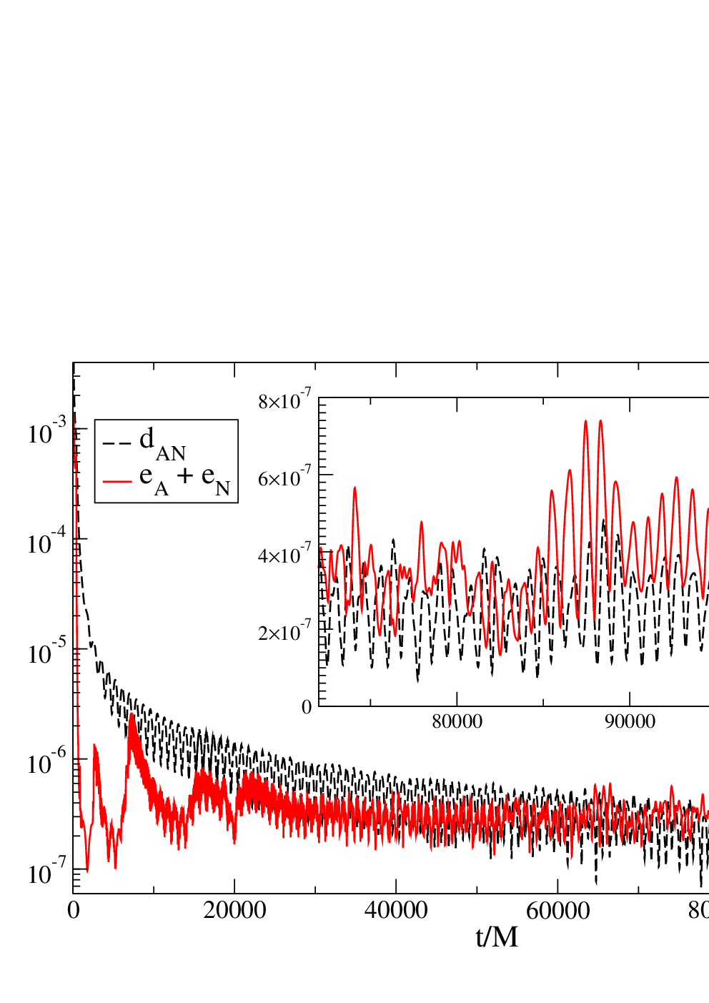
To perform a more quantitative comparison it is convenient to first do an error estimation for each case. For a semianalytical solution obtained from the first $m$ modes, $\Psi_{\rm A}(t,r)=\sum_{n=1}^{m}\Psi_{n}(t,r)$ , we estimate the error as the last term in the series. For a numerical evolution with resolution $\Delta r$ , $\Psi_{\rm N}(t,r)=\Psi_{\Delta r}(t,r)$ , we estimate the error as the difference with a solution with resolution $2\Delta r$ . In order to do a comparison in time, we take the $L^{2}$ norm in $r$ of the difference between the analytical and numerical solutions and their respective errors: $d_{\rm AN}(t):=||\Psi_{\rm A}(t,r)-\Psi_{\rm N}(t,r)||$ , $e_{\rm A}(t):=||\Psi_{m}(t,r)||$ , $e_{\rm N}(t):=||\Psi_{\Delta r}(t,r)-\Psi_{2\Delta r}(t,r)||$ . We consider that a good agreement up to numerical error is achieved whenever $d_{\rm AN}\lesssim e_{\rm A}+e_{\rm N}$ . These quantities are shown in Fig. 11 for the same cases shown in the previous figures, that is $m=9$ and $\Delta r=0.1M$ in the inner grid. As expected, we see good agreement only at late times, when the semianalitycal solution becomes a good approximation. Note that these error estimations can be considered when deciding where to stop the semianalitical series. For the results presented in this work the error $e_{\rm A}$ is of the order of 1% at the later times shown.

VI Possible observational features

There has been some recent interest in the possibility that dark matter may be described by the coherent excitation of a massive scalar field [9, 10, 11, 12, 13, 14, 15, 16, 17, 18, 19, 20, 21, 22, 23, 24, 25, 26, 27, 28]. In the axiverse [1, 2, 3, 4, 5, 6, 7, 8], scalar fields with masses in the range $10^{-33}$ to $10^{-10}$ eV might naturally appear. It is very interesting that precision black hole physics can be used to explore such a possibility [3, 5, 6]. In this section we speculate about some further astrophysical observables that can be easily computed from the results in this paper.

The semianalytic method presented in Sec. IV (and tested against numerical evolutions in Sec. V) offers interesting possibilities. Among them, it allows the evaluation of the scalar field at any time $t$ without the need of a full numerical evolution, as long as $t$ is large enough such that the contribution of the high-frequency arc vanishes.¹¹ 1 At very large times, the tail contribution to the integral kernel could in principle have some relevance [68, 69], but it does not appear for the time scales of our simulations; see Sec. III.4 for similar results in the case of the toy model. This allows us to study efficiently the amount of scalar field that “survives” around the black hole in the form of the superposition of quasi-bound modes that are excited by the initial data. We have referred to these remaining scalar field configurations as Schwarzschild scalar wigs [33]. Furthermore, we can estimate the size of these wigs by estimating the size of each quasi-bound mode. Note that even a narrow initial data, with a width of just $4M$ , can excite a large number of modes. Most of them, as shown in Fig. 6, have radial extension of hundreds or thousands of $M$ .

In order to obtain a rough estimate on the size of the quasi-bound modes,²² 2 A more precise definition would be to determine the radius of a sphere containing, let us say, 99% of the mass. we can calculate the location of the local minimum, $r_{\rm min}$ , of the effective potential $V(r)$ defined in Eq. (37). Since the actual size is usually much larger [32], this value gives a lower bound for the size of the scalar wig. Fig. 12 shows $r_{\rm min}$ as a function of $\mu$ for $\ell=0$ and $\ell=1$ , and black hole masses of order $M=10^{8}M_{\odot}$ . Larger values of $\ell$ give larger values of $r_{\rm min}$ . The values shown in Fig. 12 seem to be consistent with galactic halos. For $\ell>0$ we obtain sizes larger than those of the typical visible part of galaxies. For the case with $\ell=0$ , although the size seems too small, let us emphasize that $r_{\min}$ is usually much smaller than the actual size. Moreover, even if the modes with $\ell=0$ were smaller than the typical size of actual galactic halos, in order to describe a galaxy one would actually have to consider combinations of modes with different values of $\ell$ for a more realistic scenario, hence yielding larger sizes.

Concerning the amount of scalar field in one of those wigs, we will compute now the total energy, $E(t)$ , contained in a slice $t=\textrm{const}$ [32]. For the particular case of the Klein-Gordon equation in ingoing Eddington-Finkelstein coordinates it can be shown that

	$\displaystyle E(t)$	$\displaystyle=$	$\displaystyle\int\limits_{2M}^{\infty}\left[\left(1+\frac{2M}{r}\right)\left\|\frac{\partial\phi}{\partial t}\right\|^{2}+\left(1-\frac{2M}{r}\right)\left\|\frac{\partial\phi}{\partial r}\right\|^{2}\right.$		(51)
			$\displaystyle\qquad\left.+\left(\frac{\ell(\ell+1)}{r^{2}}+\frac{2M}{r^{3}}+\mu^{2}\right)\|\phi\|^{2}\right]dr\,.$		(51)

At late times the scalar field can be written as a superposition of quasi-bound states, $\phi(t,r)=\sum_{n}A_{n}e^{s_{n}t}\phi_{n}(r)$ , where the mode solutions in Eddington-Finkelstein coordinates $\phi_{n}(r)$ are related to the mode functions $f_{-}(s_{n},x)$ defined in Eq. (41) through the relation $\phi_{n}(r)=(r/2M-1)^{-2Ms_{n}}f_{-}(s_{n},z)$ ; see Appendix A. Given the properties of the Heun function, it follows that $\lim_{r\to 2M}\phi_{n}(r)=1$ . Using these identities and integration by parts, it can be shown that the energy in Eq. (51) can be rewritten as

E_{\textrm{modes}}(t)=-2\sum_{n,m}e^{(s_{n}^{*}+s_{m})t}\frac{s_{n}^{*}s_{m}}{s_{n}^{*}+s_{m}}A_{n}^{*}A_{m}\,.

(52)

Therefore, at late times the total energy of the scalar field can be computed solely from the quasi-bound frequencies and the excitation amplitudes corresponding to a given initial data. For the particular case of the initial data defined in Eq. (48) (with $R_{1}=4M$ and $R_{2}=8M$ ), we have computed the energy $E_{\textrm{modes}}(t)$ given in Eq. (52) for large times, $t>10,000M$ , and compared it to the initial energy, $E_{0}$ , which was computed from the integral in Eq. (51). The evolution of the normalized energy $E_{\textrm{modes}}(t)/E_{0}$ for the same initial data but different values of $M\mu$ is shown in Fig. 13.

The following comments on the behavior of $E_{\textrm{modes}}(t)/E_{0}$ are interesting. In contrast to the evolution of the energy shown in Ref. [32], where only one quasi-bound state was evolved and an exponential decay was obtained, for the case of an arbitrary data the behavior of $E(t)/E_{0}$ shows transitions from one exponential decaying phase to another one. This is due to the fact that at late times, the solution is a superposition of different quasi-bound states. However, note that the energy $E_{\textrm{modes}}(t)$ is a non-increasing function of time, since the time derivative of the right-hand side of Eq. (52) is equal to $-2$ times a perfect square. Another interesting property is that for given initial data, the amount of energy of the scalar field is initially smaller but lasts for a larger time when $M\mu$ is decreased. The reason for this relies in the fact that when $M\mu\to 0$ , the real parts of the complex frequencies $s_{n}$ , giving rise to the decay of the solution, become very small, so that the configuration can last for a longer time.

The profile in the energy density $\rho_{nlm}(t,r)$ of each individual mode $\phi_{nlm}$ is of the form shown in Figs. 6 and 7, Ref. [32]. However, the energy density of a combination of modes with different frequencies will have nontrivial oscillations, due to its nonlinear dependency on the scalar field. Assuming that galactic halos are described by a combination of these modes, such oscillations might be observable, producing changes in the galactic rotation curves over time.

Let us consider a combination of modes with two frequencies, $\omega_{1}$ and $\omega_{2}$ . The energy density will be given by the sum of the energy density of each mode (a quasi-static term), plus a cross term (given the quadratic form of the density as function of the scalar field) with frequency $\omega_{r}=\left|\omega_{1}-\omega_{2}\right|$ .

In general, the maximum possible frequency $\omega_{r}$ will then be given by the difference of the higher and lower frequencies. This value will be approximately equal to the upper bound given by the size of the resonance region: ${\omega_{b}}^{2}={\rm min}\left\{\mu^{2},V_{\rm max}\right\}-V_{\rm min}$ , where $V_{\rm max}$ ( $V_{\rm min}$ ) is the local maximum (minimum) of the effective potential $V(r)$ . In terms of periods, we have the lower bound $T_{b}=2\pi/\omega_{b}$ .

In order to give some estimations, if we choose $M=10^{10}M_{\odot}$ , $\mu=10^{-22}$ eV, and $\ell=0$ , we have $T_{b}=17$ years, thus in this case it seems plausible to detect the oscillations by, for instance, comparing rotation curves observed during a few decades of observation. This relatively small value of $T_{b}$ is obtained for minimum $\ell$ , and large $M$ and $\mu$ , although still within acceptable limits for galactic halos. However, as soon as we choose slightly smaller $M$ or $\mu$ , or larger $\ell$ , the period $T_{b}$ gets extremely larger. For example, $M=10^{8}M_{\odot}$ , $\mu=10^{-23}$ eV and $\ell=0$ gives $T_{b}=5500$ years; $M=10^{5}M_{\odot}$ , $\mu=10^{-22}$ eV and $\ell=1$ gives $T_{b}=10^{11}$ years. Thus, it remains unclear whether the oscillations might be observed.

VII Conclusions

We have considered the late time behavior of localized scalar field configurations surrounding a Schwarzschild black hole, using both numerical evolutions and the Green’s function representation technique. At any time in the evolution, the scalar field can be represented as the convolution of the initial data with a suitable integral kernel. The integral kernel can be divided into three different contributions, where each one is a contour integral in the complex frequency plane over the Green’s function of the problem. After some transient initial period, and for the time scales reached with our numerical evolutions, we have shown that the scalar field can be accurately described by a superposition of quasi-bound modes alone, which correspond to the residua of the poles of the Green’s function.

Given arbitrary initial data for the scalar field on a spacelike hypersurface, the amplitude of each quasi-bound state in the solution can be obtained by computing a simple, one-dimensional integral. Therefore, once these amplitudes have been calculated, it is possible to predict the late time behavior of the scalar field distribution without performing a numerical evolution.

These conclusions were reached by applying the Green’s function technique first to a toy model consisting of a potential formed by a delta and a step function, where the modes can be computed in exact form, and where the asymptotic form of the frequencies and the amplitudes can be obtained analytically. In particular, we showed that for this model problem all the poles of the Green’s function are located very close to the resonant band, and thus have very small decay rates. By comparison with a numerical evolution we showed that at late times the solution is accurately described by a superposition of quasi-bound modes. Then, we turned to the case of a massive scalar field on a Schwarzschild black hole background, for which the quasi-bound frequencies, modes and amplitudes were determined semianalytically, and showed that in this case too the agreement with the numerical evolutions at late times is remarkable.

We discussed some of the astrophysical implications of our findings, in particular to the scalar field dark matter models and to the axiverse. We corroborated the results in our previous works, where we found that for appropriate values of the scalar field and the black hole mass the quasi-bound states can be extremely long lived. We also estimated the size of the wigs for supermassive black holes, and speculated about a possible observational feature in the rotational curves of galaxies.

Although the method presented in this paper has been applied only to the case of a massive scalar field living on a Schwarzschild spacetime background, it can be naturally extended to higher order spin fields on other stationary spacetime geometries.

Acknowledgements.

The authors are grateful to Sam Dolan for helpful suggestions. This work was supported in part by CONACyT through grants 82787, 101353, 167335, 182445, and by DGAPA-UNAM through grants IN115311 and IN103514. AB and MM acknowledge support from CONACyT-México. JCD also acknowledges support from CONACyT-México, and from FCT via project No. PTDC/FIS/116625/2010 and NRHEPÐ295189 FP7-PEOPLE-2011-IRSES. OS was supported by a CIC grant to Universidad Michoacana de San Nicolás de Hidalgo. MM was also supported by a grant from the John Templeton Foundation. The opinions expressed in this publication are those of the authors and do not necessarily reflect the views of the John Templeton Foundation.

Appendix A Green’s function representation for arbitrary time slices

In this appendix we generalize the integral representation (2) for the solutions of Eq. (1a) to arbitrary spacelike foliations $\overline{t}=\textrm{const.}$ , where the new time coordinate $\overline{t}$ parametrizing the new foliation is related to $t$ through

\overline{t}=t-h(x),

(53)

with $h:\mathbb{R}\to\mathbb{R}$ the height function. $h$ should be smooth and satisfy $|h^{\prime}(x)|<1$ in order to ensure that the time slices $\overline{t}=\textrm{const.}$ are spacelike. With respect to the new coordinates $(\overline{t},r)$ Eq. (1a) is transformed into the following equation for $\overline{\phi}(\overline{t},x)=\phi(t,x)$ .

\frac{\partial^{2}\overline{\phi}}{\partial\overline{t}^{2}}-\left(\frac{\partial}{\partial x}-h^{\prime}(x)\frac{\partial}{\partial\overline{t}}\right)^{2}\overline{\phi}+V(x)\overline{\phi}=0.

We solve this equation given initial data on the initial surface $\overline{t}=0$ which is of the form

\overline{\phi}(0,x)=\overline{\phi_{0}}(x),\quad\frac{\partial\overline{\phi}}{\partial t}(0,x)=\overline{\pi_{0}}(x),\quad x\in\mathbb{R}.

To do this, we perform a Laplace transformation in time, which yields the ordinary differential equation

\left[s^{2}-\left(\frac{\partial}{\partial x}-h^{\prime}(x)s\right)^{2}+V(x)\right]\tilde{\phi}(s,x)=F(s,x),

(54)

where $\tilde{\phi}(s,x)$ refers to the Laplace transformation of $\overline{\phi}(\overline{t},x)$ and the source term is given by

	$\displaystyle F(s,x)$	$\displaystyle=$	$\displaystyle(1-h^{\prime}(x)^{2})(\overline{\pi_{0}}(x)+s\overline{\phi_{0}}(x))$
		$\displaystyle+$	$\displaystyle 2h^{\prime}(x)\frac{\partial\overline{\phi_{0}}}{\partial x}(x)+h^{\prime\prime}(x)\overline{\phi_{0}}(x).$

The solution of Eq. (54) which is well-behaved at $x\to\pm\infty$ can be written as

\tilde{\phi}(s,x)=\int\limits_{-\infty}^{\infty}\overline{G}(s,x,y)F(s,y)dy,

with the Green’s function

\overline{G}(s,x,y):=\frac{1}{\overline{W}(s,y)}\left\{\begin{array}[]{ll}\overline{f_{-}}(s,y)\overline{f_{+}}(s,x),&y\leq x\\ \overline{f_{-}}(s,x)\overline{f_{+}}(s,y),&y>x\end{array}\right\},

(55)

where here $\overline{f_{-}}(s,x)$ and $\overline{f_{+}}(s,x)$ are two nontrivial homogeneous solutions of Eq. (54), with $\overline{f_{-}}$ representing an outgoing mode at $x\to-\infty$ and $\overline{f_{+}}$ and outgoing mode at $x\to+\infty$ . $\overline{W}(s,x)$ is the Wronski determinant of $\overline{f}_{\pm}$ , defined as

\overline{W}(s,x):=\det\left(\begin{array}[]{ll}\overline{f_{+}}(s,x)&\overline{f_{-}}(s,x)\\ \overline{f_{+}}^{\prime}(s,x)&\overline{f_{-}}^{\prime}(s,x)\end{array}\right).

What is the relation between $\overline{G}(s,x,y)$ and the Green’s function $G(t,x,y)$ corresponding to the original time slices $t=\textrm{const.}$ ? Because of Eq. (53) the mode solutions $\overline{f_{\pm}}$ and $f_{\pm}$ are related to each other through

\overline{f_{\pm}}(s,x)=e^{sh(x)}f_{\pm}(s,x).

Accordingly, it follows that $\overline{W}(s,x)=e^{2sh(x)}W(s)$ and $\overline{G}(s,x,y)=e^{s(h(x)-h(y))}G(s,x,y)$ . With these observations, it is not difficult to generalize the formulae (8) to the case where the initial data is specified on the $\bar{t}=0$ surface instead of the $t=0$ surface. The result is

\overline{\phi}_{\textrm{modes},n}(\bar{t},x)=\overline{A_{n}}e^{s_{n}t}f_{+}(s_{n},x)=\overline{A_{n}}e^{s_{n}\overline{t}}\overline{f_{+}}(s_{n},x),

(56)

with the amplitude

\overline{A_{n}}:=\left.\left[\frac{d}{ds}W(s)\right]^{-1}\right|_{s=s_{n}}\int\limits_{-\infty}^{\infty}f_{-}(s_{n},y)e^{-s_{n}h(y)}F(s_{n},y)dy.

(57)

Comparing with Eqs. (8) we see that the only change required for computing the mode solution is the replacement $[s_{n}\phi_{0}(y)+\pi_{0}(y)]\mapsto e^{-s_{n}h(y)}F(s_{n},y)$ in the expression for the amplitude $A_{n}$ .

As an example, for ingoing Eddington-Finkelstein coordinates we have with $r>2M$ ,

x=r+2M\log\left(\frac{r}{2M}-1\right),\qquad h(x)=r-x,

and

			$\displaystyle F(s,x)dx$
		$\displaystyle=$	$\displaystyle\left[\left(1+\frac{2M}{r}\right)(\overline{\pi_{0}}+s\overline{\phi_{0}})-\frac{4M}{r}\frac{\partial\overline{\phi_{0}}}{\partial r}+\frac{2M}{r^{2}}\overline{\phi_{0}}\right]dr.$

Appendix B Contributions from the high-frequency arc and the branch cut to the solution of the toy model

In Sec. III we provided an analytic derivation of the mode part of the solutions to the toy model problem. In this appendix, we briefly discuss some properties of the remaining parts of the solution, namely the ones coming from the integration over the high-frequency arc $\mu_{R}$ and the two curves $\Gamma_{R}$ around the branch cut (see Fig. 1). The corresponding integral kernels are given by

k_{\textrm{tail}}(t,x,y)=\lim\limits_{R\to\infty}\frac{1}{2\pi i}\int\limits_{\Gamma_{R}}e^{st}G(s,x,y)ds,

and

k_{\textrm{hfa}}(t,x,y)=\lim\limits_{R\to\infty}\frac{1}{2\pi i}\int\limits_{\mu_{R}}e^{st}G(s,x,y)ds.

In terms of the complex angle $\varphi$ defined in Eq. (25) we can parametrized the integration curves $\Gamma_{R}$ and $\mu_{R}$ as follows. Let $\varepsilon>0$ and $R>0$ . Then, $\Gamma_{R}$ is defined as the union of the two hyperbolae $\varphi=\alpha+i\beta$ with $-R\leq\beta\leq R$ and $\alpha=\pm(\pi/2-\varepsilon)$ , respectively, and $\mu_{R}$ as the elliptic arc described $\varphi=\alpha+iR$ with $-\pi/2+\varepsilon\leq\alpha\leq\pi/2-\varepsilon$ , see Fig. 2. As in Sec. III, we assume that the initial data is supported inside the potential well, $0<x<a$ , and we only consider the solution inside this region. Then, the Green’s function $G(s,x,y)$ can be computed using Eqs. (4,13a–13d). In terms of the complex angle $\varphi$ one obtains:

\displaystyle e^{st}G(s,x,y)ds=\frac{(1+\lambda i\sin\varphi)e^{i\sin\varphi(\tau-\eta)}+e^{i\sin\varphi(\tau+\eta-2q)-2i\varphi}-(1+\lambda i\sin\varphi)e^{i\sin\varphi(\tau+\xi-2q)-2i\varphi}-e^{i\sin\varphi(\tau-\xi)}}{2\tan(\varphi)F(\lambda,\varphi)}d\varphi,

where we have introduced the dimensionless quantities $\tau:=\mu t$ , $\xi:=\mu(x+y)$ , $\eta:=\mu|x-y|$ , and where we recall the definitions $\lambda:=2\mu/A$ and $q:=a\mu$ and the function $F(\lambda,\varphi)$ defined in Eq. (26).

Explicit evaluation of the resulting integrals is, of course, a non-trivial task. However, we prove the following result which shows that the contribution from the high-frequency arc vanishes identically after two crossing times of the potential well:

Proposition 1

Let $t>2a$ . Then, $k_{\textrm{hfa}}(t,x,y)=0$ for all $0<x,y<a$ .

Proof. We start with a basic estimate for the function $F(\lambda,\varphi)=1+i\lambda\sin(\varphi)-e^{-2i\varphi-2qi\sin\varphi}$ . Writing $\varphi=\alpha+i\beta$ with $-\pi/2<\alpha<\pi/2$ and $\beta>0$ we have

i\sin\varphi=-\cos\alpha\sinh\beta+i\sin\alpha\cosh\beta,

which has negative real part. Using the estimates $\sinh\beta\leq e^{\beta}$ and $\cosh\beta\leq e^{\beta}$ which are valid for $\beta>0$ we obtain from this

|i\sin\varphi|=\sqrt{\cos^{2}\alpha\sinh^{2}\beta+\sin^{2}\alpha\cosh^{2}\beta}\leq e^{\beta}.

On the other hand,

-2i\varphi-2qi\sin\varphi=2\beta+2q\cos\alpha\sinh\beta-2i(\alpha+q\sin\alpha\cosh\beta)

which implies

|e^{-2i\varphi-2qi\sin\varphi}|=e^{2\beta+2q\cos\alpha\sinh\beta}\geq e^{2\beta}.

Therefore, if follows that

|F(\lambda,\varphi)|\geq e^{2\beta}-|1+i\lambda\sin\varphi|\geq e^{2\beta}-\lambda e^{\beta}-1,

(58)

and choosing $R>0$ large enough, we have $|F(\lambda,\varphi)|\geq e^{2\beta}/2$ for all $\beta\geq R$ . In particular, this proves that there are no poles which lie arbitrarily far from the origin in the complex plane.

Next, we observe that

\frac{1}{|\tan^{2}(\varphi)|}=\frac{\cosh^{2}\beta-\sin^{2}\alpha}{\sinh^{2}\beta+\sin^{2}\alpha}\leq\frac{\cosh^{2}\beta}{\sinh^{2}\beta}.

The right-hand side converges to one for $\beta\to\infty$ , implying that $1/|\tan(\varphi)|$ is uniformly bounded for large $\beta$ ’s.

Now that we have control on the terms in the denominator, it is not difficult to estimate each term of the Green’s function. For example, for the first term we find

			$\displaystyle\left\|\int\limits_{\mu_{R}}\frac{(1+\lambda i\sin\varphi)e^{i\sin\varphi(\tau-\eta)}}{2\tan(\varphi)F(\lambda,\varphi)}d\varphi\right\|$
		$\displaystyle\leq$	$\displaystyle\textrm{const}\times e^{R}e^{-2R}\int\limits_{-\pi/2+\varepsilon}^{\pi/2-\varepsilon}e^{-\cos\alpha\sinh(R)(\tau-\eta)}d\alpha$
		$\displaystyle\underset{R\to\infty}{\longrightarrow}$	$\displaystyle 0,$

since $\tau-\eta=\mu(t-|x-y|)>0$ . The second and fourth terms can be estimated in a similar way. For the third term we obtain

			$\displaystyle\left\|\int\limits_{\mu_{R}}\frac{(1+\lambda i\sin\varphi)e^{i\sin\varphi(\tau+\xi-2q)-2i\varphi}}{2\tan(\varphi)F(\lambda,\varphi)}d\varphi\right\|$
		$\displaystyle\leq$	$\displaystyle\textrm{const}\times e^{R}e^{-2R}\int\limits_{-\pi/2+\varepsilon}^{\pi/2-\varepsilon}e^{-\cos\alpha\sinh(R)(\tau+\xi-2q)+2R}d\alpha$
		$\displaystyle\leq$	$\displaystyle\textrm{const}\times 2\sinh(R)\int\limits_{-\pi/2+\varepsilon}^{\pi/2-\varepsilon}e^{-\cos\alpha\sinh(R)(\tau+\xi-2q)}d\alpha.$

In the limit $R\to\infty$ this term also converges to zero. This can be seen by setting $z:=\sinh(R)(\tau+\xi-2q)=\sinh(R)\mu(t+x+y-2a)>0$ and using the estimate $\cos\alpha\geq 1-2\alpha/\pi$ , $\alpha\geq 0$ , such that

	$\displaystyle z\int\limits_{-\pi/2+\varepsilon}^{\pi/2-\varepsilon}e^{-z\cos\alpha}d\alpha$	$\displaystyle\leq$	$\displaystyle 2z\int\limits_{0}^{\pi/2-\varepsilon}e^{-z(1-2\alpha/\pi)}d\alpha$
		$\displaystyle=$	$\displaystyle\pi\left(e^{-2\varepsilon z/\pi}-e^{-z}\right)\underset{R\to\infty}{\longrightarrow}0.$

This concludes the proof of the proposition.

References

[1] Asimina Arvanitaki, Savas Dimopoulos, Sergei Dubovsky, Nemanja Kaloper, and John March-Russell. String Axiverse. Phys.Rev., D81:123530, 2010.
[2] Bobby Samir Acharya, Konstantin Bobkov, and Piyush Kumar. An M Theory Solution to the Strong CP Problem and Constraints on the Axiverse. JHEP, 1011:105, 2010.
[3] Asimina Arvanitaki and Sergei Dubovsky. Exploring the String Axiverse with Precision Black Hole Physics. Phys.Rev., D83:044026, 2011.
[4] David J.E. Marsh. The Axiverse Extended: Vacuum Destabilisation, Early Dark Energy and Cosmological Collapse. Phys.Rev., D83:123526, 2011.
[5] Hideo Kodama and Hirotaka Yoshino. Axiverse and Black Hole. Int.J.Mod.Phys.Conf.Ser., 7:84–115, 2012.
[6] Caio F.B. Macedo, Paolo Pani, Vitor Cardoso, and Luís C.B. Crispino. Into the lair: gravitational-wave signatures of dark matter. Astrophys.J., 774:48, 2013.
[7] David J. E. Marsh, Daniel Grin, Renée Hlozek, and Pedro G. Ferreira. Axiverse cosmology and the energy scale of inflation. Phys.Rev., D87:121701, 2013.
[8] Hiroyuki Tashiro, Joseph Silk, and David J. E. Marsh. Constraints on primordial magnetic fields from CMB distortions in the axiverse. 2013.
[9] Michael S. Turner. Coherent Scalar Field Oscillations in an Expanding Universe. Phys. Rev., D28:1243, 1983.
[10] Sang-Jin Sin. Late time cosmological phase transition and galactic halo as Bose liquid. Phys. Rev., D50:3650–3654, 1994.
[11] P. J. E. Peebles and A. Vilenkin. Noninteracting dark matter. Phys. Rev., D60:103506, 1999.
[12] P. J. E. Peebles. Fluid dark matter. 2000.
[13] Varun Sahni and Li-Min Wang. A New cosmological model of quintessence and dark matter. Phys. Rev., D62:103517, 2000.
[14] Wayne Hu, Rennan Barkana, and Andrei Gruzinov. Fuzzy Cold Dark Matter: The wave properties of ultralight particles. Phys. Rev. Lett., 85:1158–1161, 2000.
[15] Tonatiuh Matos and L. Arturo Urena-Lopez. Quintessence and scalar dark matter in the universe. Class. Quant. Grav., 17:L75–L81, 2000.
[16] Tonatiuh Matos and L. Arturo Urena-Lopez. A further analysis of a cosmological model of quintessence and scalar dark matter. Phys. Rev., D63:063506, 2001.
[17] Alexandre Arbey, Julien Lesgourgues, and Pierre Salati. Quintessential haloes around galaxies. Phys. Rev., D64:123528, 2001.
[18] Tonatiuh Matos, Argelia Bernal, and Dario Nunez. Flat Central Density Profiles from Scalar Field Dark Matter Halo. Rev.Mex.A.A., 44:149, 2008.
[19] Jae-Weon Lee and Sooil Lim. Minimum mass of galaxies from BEC or scalar field dark matter. JCAP, 1001:007, 2010.
[20] P. Sikivie and Q. Yang. Bose-Einstein Condensation of Dark Matter Axions. Phys.Rev.Lett., 103:111301, 2009.
[21] David J. E. Marsh and Pedro G. Ferreira. Ultra-Light Scalar Fields and the Growth of Structure in the Universe. Phys. Rev., D82:103528, 2010.
[22] Andrew P. Lundgren, Mihai Bondarescu, Ruxandra Bondarescu, and Jayashree Balakrishna. Lukewarm dark matter: Bose condensation of ultralight particles. Astrophys. J., 715:L35, 2010.
[23] Kung-Yi Su and Pisin Chen. Solving the Cusp-Core Problem with a Novel Scalar Field Dark Matter. 2010.
[24] F. Briscese. Viability of complex self-interacting scalar field as dark matter. Phys. Lett., B696:315–320, 2011.
[25] T. Harko. Bose-Einstein condensation of dark matter solves the core/cusp problem. JCAP, 1105:022, 2011.
[26] V. Lora, Juan Magana, Argelia Bernal, F.J. Sanchez-Salcedo, and E.K. Grebel. On the mass of ultra-light bosonic dark matter from galactic dynamics. JCAP, 1202:011, 2012.
[27] Alma X. Gonzalez-Morales, Alberto Diez-Tejedor, L. Arturo Urena-Lopez, and Octavio Valenzuela. Hints on halo evolution in SFDM models with galaxy observations. Phys.Rev., D87:021301, 2013.
[28] Tanja Rindler-Daller and Paul R. Shapiro. Complex scalar field dark matter on galactic scales. 2013.
[29] Laura Ferrarese and David Merritt. A Fundamental relation between supermassive black holes and their host galaxies. Astrophys.J., 539:L9, 2000.
[30] J. D. Bekenstein. Novel ’no scalar hair’ theorem for black holes. Phys. Rev., D51:6608–6611, 1995.
[31] I. Pena and D. Sudarsky. Do collapsed boson stars result in new types of black holes? Class. Quant. Grav., 14:3131–3134, 1997.
[32] Juan Barranco, Argelia Bernal, Juan Carlos Degollado, Alberto Diez-Tejedor, Miguel Megevand, et al. Are black holes a serious threat to scalar field dark matter models? Phys.Rev., D84:083008, 2011.
[33] Juan Barranco, Argelia Bernal, Juan Carlos Degollado, Alberto Diez-Tejedor, Miguel Megevand, et al. Schwarzschild black holes can wear scalar wigs. Phys.Rev.Lett., 109:081102, 2012.
[34] I.M. Ternov, V.R. Khalilov, G.A. Chizhov, and Alex B. Gaina. Finite movement of massive particles in kerr and schwarzschild fields. Sov.Phys.J., 21:1200–1204, 1978.
[35] Akira Ohashi and Masa-aki Sakagami. Massive quasi-normal mode. Class.Quant.Grav., 21:3973–3984, 2004.
[36] Julien Grain and A. Barrau. Quantum bound states around black holes. Eur.Phys.J., C53:641–648, 2008.
[37] S. Detweiler. Klein-gordon equation and rotating black holes. Phys. Rev., D22:2323, 1980.
[38] Sam R. Dolan. Instability of the massive Klein-Gordon field on the Kerr spacetime. Phys.Rev., D76:084001, 2007.
[39] Horst R. Beyer. On the stability of the Kerr metric. Commun.Math.Phys., 221:659–676, 2001.
[40] Horst Reinhard Beyer. On the stability of the massive scalar field in Kerr space-time. J.Math.Phys., 52:102502, 2011.
[41] Horst Reinhard Beyer, Miguel Alcubierre, Miguel Megevand, and Juan Carlos Degollado. Stability study of a model for the Klein-Gordon equation in Kerr spacetime. Gen.Rel.Grav., 45:203–227, 2013.
[42] Yakov Shlapentokh-Rothman. Exponentially growing finite energy solutions for the Klein-Gordon equation on sub-extremal Kerr spacetimes. 2013.
[43] Helvi Witek, Vitor Cardoso, Akihiro Ishibashi, and Ulrich Sperhake. Superradiant instabilities in astrophysical systems. Phys.Rev., D87:043513, 2013.
[44] Sam R. Dolan. Superradiant instabilities of rotating black holes in the time domain. Phys.Rev., D87:124026, 2013.
[45] Hirotada Okawa, Helvi Witek, and Vitor Cardoso. Black holes and fundamental fields in Numerical Relativity: initial data construction and evolution of bound states. 2014.
[46] E.W. Leaver. An Analytic representation for the quasi normal modes of Kerr black holes. Proc.Roy.Soc.Lond., A402:285–298, 1985.
[47] R. A. Konoplya and A. V. Zhidenko. Decay of massive scalar field in a Schwarzschild background. Phys. Lett., B609:377–384, 2005.
[48] Hironobu Furuhashi and Yasusada Nambu. Instability of massive scalar fields in Kerr-Newman space-time. Prog.Theor.Phys., 112:983–995, 2004.
[49] Anthony Lasenby, Chris Doran, Jonathan Pritchard, Alejandro Caceres, and Sam Dolan. Bound states and decay times of fermions in a Schwarzschild black hole background. Phys.Rev., D72:105014, 2005.
[50] Joao G. Rosa and Sam R. Dolan. Massive vector fields on the Schwarzschild spacetime: quasi-normal modes and bound states. Phys.Rev., D85:044043, 2012.
[51] Luis Arturo Urena-Lopez and Andrew R. Liddle. Supermassive black holes in scalar field galaxy halos. Phys. Rev., D66:083005, 2002.
[52] Alejandro Cruz-Osorio, F. Siddhartha Guzman, and Fabio D. Lora-Clavijo. Scalar Field Dark Matter: behavior around black holes. JCAP, 1106:029, 2011.
[53] L. Arturo Urena-Lopez and Lizbeth M. Fernandez. Black holes and the absorption rate of cosmological scalar fields. 2011.
[54] F.S. Guzman and F.D. Lora-Clavijo. Spherical non-linear absorption of cosmological scalar fields onto a black hole. Phys.Rev., D85:024036, 2012.
[55] Xiang-Nan Zhou, Xiao-Long Du, Ke Yang, and Yu-Xiao Liu. Dirac dynamical resonance states around Schwarzschild black holes. 2013.
[56] Edward W. Leaver. Spectral decomposition of the perturbation response of the Schwarzschild geometry. Phys.Rev., D34:384–408, 1986.
[57] T.J.M. Zouros and D.M. Eardley. Instabilities of massive scalar perturbations of a rotating black hole. Annals Phys., 118:139–155, 1979.
[58] Paolo Pani, Vitor Cardoso, Leonardo Gualtieri, Emanuele Berti, and Akihiro Ishibashi. Perturbations of slowly rotating black holes: massive vector fields in the Kerr metric. Phys.Rev., D86:104017, 2012.
[59] Hirotaka Yoshino and Hideo Kodama. Bosenova collapse of axion cloud around a rotating black hole. Prog.Theor.Phys., 128:153–190, 2012.
[60] Hirotaka Yoshino and Hideo Kodama. Gravitational radiation from an axion cloud around a black hole: Superradiant phase. 2013.
[61] Hans-Peter Nollert. Topical Review: Quasinormal modes: the characteristic ‘sound’ of black holes and neutron stars. Class.Quant.Grav., 16:R159–R216, 1999.
[62] K. Kokkotas and B. Schmidt. Quasi-normal modes of stars and black holes. Living Rev. Rel., 3:5, 1999.
[63] Emanuele Berti, Vitor Cardoso, and Andrei O. Starinets. Quasinormal modes of black holes and black branes. Class.Quant.Grav., 26:163001, 2009.
[64] M. Abramowitz and I.A. Stegun. Handbook of Mathematical Functions: with Formulas, Graphs, and Mathematical Tables. Dover Books on Mathematics. Dover Publications, 2012.
[65] A. Ronveaux and F.M. Arscott. Heun’s Differential Equations. Oxford science publications. Oxford University Press, 1995.
[66] Luis Lehner, Steven L. Liebling, and Oscar Reula. AMR, stability and higher accuracy. Class.Quant.Grav., 23:S421–S446, 2006.
[67] Miguel Megevand, Ignacio Olabarrieta, and Luis Lehner. Scalar field confinement as a model for accreting systems. Class. Quant. Grav., 24:3235–3258, 2007.
[68] Hiroko Koyama and Akira Tomimatsu. Asymptotic tails of massive scalar fields in Schwarzschild background. Phys.Rev., D64:044014, 2001.
[69] Hiroko Koyama and Akira Tomimatsu. Slowly decaying tails of massive scalar fields in spherically symmetric space-times. Phys.Rev., D65:084031, 2002.