Wavelet-Based Cascade Model for Intermittent Structure in Terrestrial Environments

Terrestrial environments, both natural and man-made, often possess complex, random spatial distributions of objects. Figures 1–6 show some illustrative examples: a volcanic crater and rock formations, an up-close view of volcanic rock, arctic melt ponds, an arctic ice floe, a turbulence simulation, and urban/suburban topography, respectively. The visual similarities of these various random heterogeneous media (RHM) are striking in several aspects, despite the very different phenomena underlying their creation. In particular, these RHM often share two traits which are focal points for this report: self-similarity and intermittency.

Realistic models of terrestrial environments have applications to many practical Army problems. In particular, this report was motivated by the desire to improve models for random atmospheric and terrain features of acoustic, seismic, and electromagnetic wave propagation calculations. The propagating waves are scattered by random inhomogeneities in the environment such as turbulence, dust, and rocks. Random fading and coherence loss in signals results, which degrades the performance of sensor systems used for detecting and localizing emitters, and for communications. The environmental modeling and wave propagation calculations may be done by theoretical (Tatarskii,, 1971; Ostashev,, 1997, e.g.,) or numerical (Anderson et al.,, 2004; Wilson et al.,, 2005, e.g.,) methods. In particular, the latter two studies demonstrated how the coupling of synthesized environmental scenes and high-fidelity wave propagation models running on parallel-processing supercomputers enables cost-effective, rapid virtual testing of new sensor systems and employment concepts.

Conventional theoretical treatments of signal propagation (Tatarskii,, 1971; Rytov et al.,, 1989; Ostashev,, 1997, e.g.,) assume that heterogeneities (terrestrial objects) responsible for random scattering of the wavefield are evenly distributed in space. This is a significant shortcoming in existing capabilities for characterizing and predicting environmental effects on system performance. Figure 7 depicts how an intermittent medium affects signal propagation. Along some paths, the waves encounter many scattering objects and signal coherence (a measure of signal randomness, which usually determines the sensing system performance) is strongly degraded. Other paths encounter relatively few scattering objects and thus have a high signal coherence. Conventional wave scattering theory assumes, in effect, that all paths experience similar scattering. It thus neglects the range of possible outcomes and related uncertainty in system performance, which, depending on the environment, can be very significant. Urban areas provide a particularly important example: optical or RF communication systems may be rendered useless by obstructions in built-up sections, whereas signals may propagate very cleanly through open areas such as large lawns and parking lots.

To address such issues, some more recent papers on acoustic and electromagnetic propagation through turbulence have considered intermittency (Hentschel and Procaccia,, 1983; Tatarskii and Zavorotnyi,, 1985; Gurvich and Kukharets,, 1986; Wilson et al.,, 1996, e.g.,). Most of these studies were based on the log-normal model for turbulent intermittency, which is known to have substantial shortcomings (Mandelbrot,, 1974). Previous theoretical treatments are also usually restricted with regard to the length of the propagation path, size of the largest inhomogeneities, wavelength, and strength of the scattering. This report, while it does not address wave propagation directly, does provide new modeling approaches for self-similar, intermittent RHM that can subsequently provide a basis for improving theoretical treatments and numerical modeling, and thus lead to more realistic characterization of the performance of Army sensing and communication systems operating in complex, real-world environments.

This report explores how concepts for self-similar cascade processes can be incorporated into the previously developed quasi-wavelet (QW) model for RHM, thus introducing realistic intermittency features into RHM modeling. QW models have been shown capable of synthesizing very realistic turbulence fields (Goedecke et al.,, 2006; Wilson et al.,, 2009, e.g.,), and were subsequently applied to surface geology (Wilson et al., 2008a, ). The approach in this report evolved out of an earlier paper presented at the Army Science Conference (Wilson et al., 2008a, ). One of the main improvements is that the three cascade reactions in the ASC paper have been replaced by a single, more general, reaction, which improves the analytical and stability properties of the model. The report also provides much additional background and a more systematic development of the model.

Section 2 provides a conceptual introduction to fractals, which serves as a foundation for the subsequent treatment of cascade processes. Next, Sec. 3 introduces self-similar QW models. A systematic and simple approach is provided for describing the scale ratios, generations, and densification of scales.

The following four sections describe the three basic model constructions: static, steady, and non-steady. The static approach, described in Sec. 4, does not explicitly incorporate evolution in time; it describes a single “snapshot” of the random medium. Next, in Sec. 5, the steady-state cascade process model is introduced, in which creation and destruction of the QWs at each scale are in equilibrium. Sec. 6 derives formulas for determining model parameters from observed statistics of an RHM. It is shown that the static and steady-state models are indistinguishable, on the basis of second-order statistics, when only a single snapshot of the process is analyzed. Lastly, a modeling approach involving explicit simulation of the cascade process, which may be used for either a steady-state or non-steady-state model, is discussed in Sec. 7.

A famous example of a fractal is the Sierpinski carpet, shown in Fig. 8.³³ 3 For reasons unknown to the present author, Mandelbrot (1977, p. 166) refers to the object in Fig. 8 as a Sierpinski carpet, whereas Schroeder (1991, p. 179) calls it a Cantor gasket. Mandelbrot’s terminology is used here. The carpet is constructed from a square. A smaller square, with side length 1/3 of the original square, is then removed from the center. This leaves 8 squares of “fabric,” each with side length 1/3 of the original, around the edges. The process is then repeated by removing squares of fabric, with side length 1/9 of the original, from the centers of each of the remaining eight squares. After many iterations of this process, one has the carpet shown in Fig. 8.

The Hausdorff (fractal) dimension can be calculated from the formula $H=\log N/\log(1/\ell)$, where $N$ is the number of new objects created from the old one each time the “measuring stick” is decreased by a factor $\ell$. In the case of the Sierpinski carpet, $N=8$ and $\ell=1/3$. Hence $H=1.893\ldots$, which is less than the topographical dimension $D=2$. If no fabric were removed at each iteration ($N=9$ and $\ell=1/3$), we would have an integer Hausdorff dimension, $H=2$, as expected for a two-dimensional object such as a square.

The Sierpinski carpet is a deterministic fractal, since it looks identical each time it is generated. It is also possible to construct random fractals. For example, we might randomize the location from which the piece of fabric is cut at each iteration. Similarly, we might specify a probability that a given piece of fabric is removed at each iteration. The result of applying this second method is shown in Fig. 9. Just like the deterministic fractal in the first example, there is an $8/9$ probability that a given sub-cell will be covered with fabric. The expected number of covered cells in the first iteration is thus $9(8/9)=8$. In the second iteration, a cell will be covered if it was covered at both the first iteration and the next. Hence the expected number of cells covered after the second iteration is $81*(8/9)*(8/9)=8^{2}$. Continuing in this fashion, it is clear that $N=8$, and hence the Hausdorff dimension is unchanged from the deterministic Sierpinski carpet.

Figures 8 and 9 demonstrate that objects with very dissimilar appearances can have the same Hausdorff dimension. Another interesting example, which bridges the gap between the purely deterministic and purely random carpets, is shown in Fig. 10. This could be called a “dirty” Sierpinski carpet. It is like the normal, deterministic carpet, except that the chance of removing any one of the eight pieces of fabric surrounding the center is $0.01$, rather than 0. To maintain an overall probability keeping 8 pieces at each iteration, we set the probability of removing the center piece to $0.92$, instead of 1. The expected value of the number of pieces retained in the first generation is thus $N_{1}=(8\cdot 0.99)+(1\cdot 0.08)=8$. At the next generation, we have $N_{2}=8\cdot 0.99[(8\cdot 0.99)+(1\cdot 0.08)]+0.08[(8\cdot 0.99)+(1\cdot 0.08)]=8^{2}$. Continuing in this fashion, we find $N=8$. Thus, the Hausdorff dimension of Fig. 10 remains the same as Fig. 8.

The examples in the previous section were all based on removing and adding square shapes. Fractals can be constructed from other shapes also. An example with randomly placed, circular cut-outs is shown in Fig. 11. Mandelbrot (1977) compared the appearance of these circular cut-outs to craters on the moon and Swiss cheese. We thus refer to the process underlying the construction of Fig. 11 as a cratering process.

The randomly placed craters (circles) in Fig. 11 have radii equal to $a_{i}=(1/3)^{i}/\sqrt{\pi}$ (where $i=1,2,\ldots$ indicates the generation of the cratering process) times the side length of the square area in which they are placed. Hence their areas are $(1/3)^{2i}$, just like the sequence of square cut-outs in Fig. 8. At each generation, $9^{i-1}$ craters are added.⁴⁴ 4 The reader may recall from the previous section that construction of the Sierpinski carpet involved $8^{i-1}$ new cut-outs at each iteration. Hence, for consistency, it might seem we should introduce $8^{i-1}$ new craters. The reason for this apparent discrepancy is that some of the craters overlap with the previous ones, and thus play essentially no role in the construction. (The construction of the Sierpinski carpet does not allow such overlap.) For example, since the first iteration produces a single crater covering $1/9$ of the total area, of the next $9$ randomly placed craters, one will on average overlap with the previous crater. This notion will be formulated more rigorously later in this section. Let us define the packing fraction as the total area of the craters for a given size class (that is, the number of craters, $N_{i}$, times the area of each, $A_{i}=\pi a_{i}^{2}$), divided by the area of the square ($A$):

$$\phi_{i}=\frac{N_{i}A_{i}}{A}.$$

(1)

In this example, $\phi_{i}=1/9$ for all $i$. Four generations are simulated ($I=4$).

The method for randomly placing the craters in Fig. 11 is based on a Poisson process. First, the overall area $A$ is partitioned into $R$ rows and $C$ columns of pixels. The area of each pixel is thus $A/RC$. The probability $p_{i}$ of the center of a circle in size class $i$ occurring within a particular pixel equals the expected number of circles of that size class divided by the number of possible locations, $N_{i}/RC=(\phi_{i}A)/(\pi a_{i}^{2}RC)=(\phi_{i}\Delta x\Delta y)/(\pi a_{i}^{2})$, where $\Delta x$ and $\Delta y$ are the grid spacing. Hence, the finer we make the grid, the smaller $p_{i}$ becomes. If $p_{i}$ is sufficiently small, the actual number of circles $n_{i}$ of size class $i$ present in realizations of the cratering process is a random variable with Poisson distribution with mean $N_{i}$, $P_{N_{i}}(n_{i}=\nu)$, where:⁵⁵ 5 The applicability of the Poisson distribution to a situation such as this is described in many introductory texts in statistics, such as Lapin (1980).

$$P_{N}(n=\nu)=\frac{N^{\nu}e^{-N}}{\nu!}.$$

(2)

Figure 12 shows this probability distribution for $N_{i}=4$ and $N_{i}=20$. For example, when $N_{i}=4$, there is a probability of about $17.5\%$ that four cut-outs will actually be present in the realization, and $0.7\%$ chance that none will be present.

Clearly, as more craters are added, the amount of remaining, uncratered area (corresponding to the fabric in the Sierpinski carpet example) decreases. After the first generation, which on average has one crater of area $1/9$, we would have approximately $8/9$ of the uncratered area remaining. If the next set of craters, of which there are $9$ each with area $1/81$, do not overlap with any other craters, we would have $8/9-9(1/81)=8/9-1/9=7/9$ of the uncratered area left. Carrying on, we would have $6/9$, then $5/9$, etc. However, this sequence cannot continue indefinitely, because eventually the assumption that there is no overlap must fail.

A more precise analysis would thus account for the overlapping of the craters. Suppose some fraction $\sigma$ of the area is uncratered after randomly placing a number of craters. This value equals the probability that a randomly selected point will be a part of the uncratered area. Next, suppose a crater from generation $i$, with fractional area $A_{i}/A$, is randomly added. The fractional area that is not a part of this crater is $1-A_{i}/A$. For a random point to fall within the uncratered area, that point must have been uncratered prior placement of the new crater, and must also be outside the new crater. The probability of both of these conditions being met is $\sigma(1-A_{i}/A)$. Carrying on in this manner, the probability of a given point remaining a part of the uncratered area, after the placement of $N_{i}$ craters of each generation (size class), is

$$\sigma=\sigma_{0}\prod_{i=1}^{I}(1-A_{i}/A)^{N_{i}},$$

(3)

where $\sigma_{0}$ is the initial uncratered fraction (normally 1) and $I$ is the number of generations (sizes) of the circles. The fractional uncratered area remaining after the addition of generation $i$ is

$$\sigma_{i}=\sigma_{0}\prod_{j=1}^{i}(1-A_{j}/A)^{N_{j}}.$$

(4)

If $\phi_{i}=N_{i}A_{i}/A\ll 1$ for all $i$, we have

$$\sigma_{i}\approx\sigma_{0}\prod_{j=1}^{i}(1-\phi_{j}).$$

(5)

This approximation amounts to neglecting the overlap between craters within each size class (but not between size classes). Finally, when $\phi_{i}$ is the same for all $i$, we have the simple result

$$\sigma_{i}\approx\sigma_{0}(1-\phi)^{i}\approx\sigma_{0}\left({1-i\phi+\frac{i(i-1)}{2}\phi^{2}-\cdots}\right).$$

(6)

Here, we use $\phi$ without a subscript to indicate the constant value for all size classes. The second approximation follows from the binomial expansion, assuming that $\phi\ll 1$. In iterative form, Eq. 6 implies

$$\sigma_{i+1}=(1-\phi)\sigma_{i}.$$

(7)

The cratered area at each iteration $\delta_{i}$, equals $1-\sigma_{i}$. One then finds $\delta_{i+1}=(1-\phi)\delta_{i}+\phi$.

Figure 13 compares the results of the cratering simulation with $\sigma_{0}=1$ and $\phi=1/9$ to Eq. 3 and the approximation, Eq. 6. A total of random 1024 cratering experiments were performed. The x’s represent the mean of these trials, and the boxes indicate the 25th, 50th (median), and 75th percentiles. For this case, Eqs. 3 and 6 both agree nearly exactly with the mean, thus indicating that the overlap between craters is statistically negligible.

A similar simulation, but with $\phi$ increased to $1/3$ to create more overlap, is shown in Figure 14. In this case, Eq. 3 still agrees well with the mean, but the approximation, Eq. 6, is no longer very accurate.

The quantiles shown in Figs. 13 and 14 indicate substantial variability in the uncratered fraction from trial to trial. Since the variability actually diminishes as more generations are added, it appears that the variability may be primarily caused by randomness in the number of the largest craters, as results from the Poisson process. Figure 15 tests this hypothesis. This figure is the same as Fig. 13, except that a single crater is always added for the first generation. The variability in the uncratered fraction thus disappears for the first generation; however, the variability remains greatly diminished as additional generations are added, thus demonstrating that most of the variability is linked to the largest craters.

Up to this point, the ratio of one size class to the next generation has always been an integer value. This is necessary for fractals generated by partitioning cells into exactly fitting sub-cells, such as in Sec. 2.1. The cells and sub-cells need not be square (or rectangular); for example, a fractal carpet built from triangles is described in Schroeder (1991). Randomly placed shapes like the circles in Fig. 11, do not need to fit together, however, so the value $1/\ell$ can readily be set to a non-integer. Figure 16 shows craters with radii $a_{i}=(1/3)^{i/4}/\sqrt{\pi}$ (where $i=1,2,\ldots$), and hence $1/\ell=a_{i}/a_{i+1}=3^{1/4}$. Because there are four times as many size classes as before, the packing fraction has been decreased to $1/36$ to produce a similar coverage in area. To the eye, the distribution of sizes appears nearly continuous, like many natural phenomena.

In the previous sections, we described the black areas in Figs. 8–10 as being “cut-outs” from the carpet fabric, whereas the white areas were the remaining fabric. The black areas in Figs. 11 and 16 were craters, whereas the white areas were uncratered. In terms of the construction process, the black areas are intended to represent area that is progressively removed from the 2D region, thus creating a fractal set. In this sense, $\sigma_{i}$ is viewed the occupied fraction, whereas $\alpha_{i}=1-\sigma_{i}$ is the void fraction. Still, if for some reason it is so preferred, the terminology and associations could be reversed. The white areas could be viewed as voids, and the black areas as objects. Then $\sigma_{i}$ would be the void fraction, and $\alpha_{i}$ the occupied fraction.

A more abstract interpretation is that the black regions become in some sense “inactive” or “disallowed” regions. This viewpoint is closer to that espoused by Mandelbrot, (1974) and Frisch et al., (1978) when they discussed the fractal properties of turbulence. Specifically, the dissipation of turbulent kinetic energy (TKE) was viewed as taking place on a fractal set embedded in a 3D volume. The dissipation surface might be conceptualized as rotating and twisting sheets. A useful intuitive analogy might be made to the construction of houses on dry land. In this analogy, the inactive region, where no housing construction is possible, consists of bodies of water. As one examines maps at a finer and finer scale, more small bodies of water, and hence inactive construction regions, become evident. This does not mean that construction is equally vigorous at all dry land locations, but rather that construction is spatially confined to these active regions.

We thus might think of the white regions in the figures as comprising the spatial support for the cascade process. Within these regions, the cascade process is fully active in some sense, whereas in the black regions it is inactive. This idea could be taken a step further, with “shades of gray” where the cascade process occurs in an intermediate state of activity. For consistency with the fractal model, the support should be created such that the active area decreases with decreasing object size. This can be done, for example, by using a cratering process to create the inactive regions cascade process. Objects of a particular size may not occur within an inactive region that is larger than the object.

As a concrete example, let us construct the support from Gaussian craters, namely

$$g_{i}(r)=\exp\left({-{r^{2}}/{a_{i}^{2}}}\right),$$

(8)

where $r$ is the distance from the center of the crater and $a_{i}$ its effective radius. (It can be shown, by integrating Eq 8 over all area, that the two-dimensional support is $\pi a_{i}^{2}$, just like the circular crater.). A value of $1$ for $g_{i}(r)$ indicates an inactive region, whereas $0$ indicates a fully active region. The inactive region for a particular size class $i$ is determined by multiplying all craters of size $i$ and larger. The active region, or support for the process, equals $1$ minus the inactive region. An example realization of such a cratering process is shown in Fig. 17. This process was constructed with the same statistical method and parameters as Fig. 11, except for the change to a Gaussian function (instead of perfect circles), and application of the just-described algebraic rules for constructing the support.

As indicated by Eq. 6 above, the active fractional area of the support is $\sigma_{i}\approx(1-\phi^{\prime})^{i-1}$ for size class $i$, where $\phi^{\prime}$ is the packing fraction of the cratering process used to create the support.⁶⁶ 6 Here it is assumed that the active region for the first size includes the entire area, i.e., $\sigma_{1}=1$. Hence the exponent $i$ in Eq. 6 is replaced by $i-1$. The packing fraction for each size class is approximately the full activity packing fraction for the objects, $\phi$, times the active fractional area. Hence, for size class $i$, $\phi_{i}\approx\phi(1-\phi^{\prime})^{i}$. In the particular example shown in Figs. 11 and 17, $\phi^{\prime}=\phi=1/9$, so $\phi_{i}\approx(1/9)(8/9)^{i}$.

Having developed a model for the support of the process, we now use this model to modulate the activity level of a second random cratering process. The previous section described the cratering process using a Poisson model, in which there is a probability $p_{i}$ of the center of a circle of size class $i$ occurring within a particular pixel. In the current context, we may regard $p_{i}$ as the probability of a crater appearing when the process is fully developed. In an inactive region, the probability drops to zero. Thus, we multiply $p_{i}$ by the value of the support, and then implement the second cratering process. Figure 18 shows the result. Qualitative intermittency effects similar to real-world random media of interest, such as the Amboy site (Fig. 2) and ice floes (Fig. 3), are now apparent.

Figures 19 and 20 are similar to 17 and 18, respectively, except that $\phi^{\prime}$ and $\phi$ have been increased to $1/3$, so $\phi_{i}\approx(1/3)(2/3)^{i}$. The result is a medium with more voids, and for which the small craters are more concentrated into smaller regions of space.

We assume for now that the parent function $f$ is spherically symmetric. That is, $f$ depends only on the magnitude $\xi$ of the vector $\boldsymbol{\xi}\equiv\left(\mathbf{r}-\mathbf{b}^{ij}\right)/a_{i}$, where $\mathbf{r}$ is the spatial coordinate, $\mathbf{b}^{ij}$ is the location of the center of the QW, and $a_{i}$ is a length scale, which can be taken as the radius of the QW, or another convenient measure. The index $i$ ($i=1,\ldots,I$) indicates the size class of the QW, with $i=1$ being the largest size (called the outer scale), and $i=I$ the smallest size (called the inner scale). The index $j$ indicates a particular QW belonging to the size class $i$. (The notational convention followed here is that a superscript $ij$ indexes a single QW, whereas a subscript $i$ indicates a property associated with all QWs of a particular size class.)

The parent function is normalized such that⁷⁷ 7 This normalization was not used in previous papers on QWs, such as Wilson et al., (2009), in which the integral of $f^{2}(\xi)$ over volume was flexible and designated as $I_{D}$. Thus, for this report, $I_{D}=1$. The normalization helps to standardize the size of the QW volume. For example, a QW in the shape of a cube, after normalization of the parent function, would have always have a volume of $V_{i}=a_{i}^{D}$ as expected.

$$\int_{V}d^{D}\xi\,f^{2}\left(\xi\right)=1.$$

(9)

The following Gaussian parent function meets this normalization condition, and is convenient for analysis and rapid calculation on computers:

$$f\left(\xi\right)=\exp\left({-\frac{\pi\xi^{2}}{2}}\right).$$

(10)

Other choices for spherically symmetric parent functions are of course possible; Goedecke et al., (2004) and Wilson et al., (2009) discuss several alternatives and their utility.

The field perturbation associated with an individual QW is written as

$$Q^{ij}\left(\mathbf{r}\right)=h^{ij}q_{i}f\left(\frac{\left|\mathbf{r}-\mathbf{b}^{ij}\right|}{a_{i}}\right),$$

(11)

where $h^{ij}$ is a random coefficient that may be positive or negative, and $q_{i}$ is an amplitude factor for the size class. (The amplitude will be associated with particular physical quantities later on.) The total scalar field $Q\left(\mathbf{r}\right)$ is then constructed by summing the contributions of each individual QW in the ensemble:⁸⁸ 8 Here we deal entirely with synthesis of scalar fields. QW models for turbulent velocity fields are discussed in Goedecke et al., (2004).

$$Q\left(\mathbf{r}\right)=\sum_{i=1}^{I}\sum_{j=1}^{N_{i}}Q^{ij}\left(\mathbf{r}\right),$$

(12)

where $N_{i}$ is the number of QWs in the size class $i$ that contribute to the field in the observation volume $V$. Volume is used here in a generic sense to indicate a $D$-dimensional region.

The quantity $V_{i}=N_{i}a_{i}^{D}$ corresponds to the total volume occupied by QWs of size $a_{i}$; hence $V_{i}/V$ is the effective fraction of $V$ occupied by QWs of size $a_{i}$. This motivates the definition of the packing fraction as

$$\phi_{i}=\frac{N_{i}a_{i}^{D}}{V}=\mathcal{N}_{i}a_{i}^{D},$$

(13)

where $\mathcal{N}_{i}=N_{i}/V$ is the number density (number per unit volume) for the size class. Note that the packing fraction is unaffected by overlap among individual QWs; it simply reflects the number of QWs in a size class per unit volume, scaled by the effective volume of QWs in that size class.

This section describes construction of a self-similar ensemble of QWs. By this, we mean that the properties of the QWs, and the rules by which the ensemble are constructed, are independent of the size class $i$. (Exceptions may be made for the largest size class, $i=1$, and the smallest, $i=I$.) We also define in this section additional quantities associated with the QWs, such as amplitudes and energies, and relate these to the length scales and number densities.

Assuming self similarity, the ratio of the scales between adjacent classes, $a_{i+1}/a_{i}$, must be independent of $i$. Thus an invariant ratio $\ell$ can be defined as follows:⁹⁹ 9 In previous formulations of QW models (Goedecke et al.,, 2006, e.g.,), the ratio $a_{i+1}/a_{i}$ was set to $e^{-\mu}$, where $\mu$ is an adjustable parameter equal to $-\ln\ell$. Adoption of $\ell$ in this paper is for convenience.

$$\ell=\frac{a_{i+1}}{a_{i}}.$$

(14)

We will later associate $\ell$ with the ratio of length scales between generations of the cascade process. In the construction of many fractals and the beta-model for turbulence (Frisch et al.,, 1978), for example, at each iteration of the construction $a_{i+1}$ is set to $a_{i}/2$, which implies $\ell=1/2$. For the time being, however, the spacing between the size classes may be regarded as arbitrary. From Eq. 14, it follows that

$$a_{i}=a_{1}\ell^{i-1}.$$

(15)

Ratios of other properties between adjacent size classes must also be invariant in order to preserve self similarity. The ratio of packing fractions between adjacent size classes, i.e.,

$$\overline{\phi}=\frac{\phi_{i+1}}{\phi_{i}}$$

(16)

is of particular interest. A decreasing packing fraction ($\overline{\phi}<1$) indicates that activity is concentrated in less volume as the size of the QWs decreases; this relates to the fractal dimension of the process.¹⁰¹⁰ 10 When $\ell=1/2$, the ratio ${\phi_{i+1}}/{\phi_{i}}$ corresponds to the parameter $\beta$ in the beta model (Frisch et al.,, 1978). Each generation in the beta model consists of halving the size of the eddies. Presuming that $\phi_{1}$ and $\overline{\phi}$ are known, we can determine the packing fractions for the remaining size classes as

$$\phi_{i}=\phi_{1}\overline{\phi}\,^{i-1}.$$

(17)

The packing fraction is related to the more commonly encountered volume fraction. The volume fraction is analogous to the fractional area occupied by the craters, as introduced in Sec. 2.3 and indicated by the symbol $\delta=1-\sigma$. The packing fraction tends to be more convenient for analysis of energetics, whereas the volume fraction is usually more convenient for comparisons with observations. For the case where the QWs are distributed uniformly and randomly over space, the relationship between the two can be derived analytically. In particular, Eqs. 3–7 apply, although we replace $A_{i}/A$ with $V_{i}/V$. (Or, we could use $\phi_{i}/N_{i}=V_{i}/V=A_{i}/A$.)

The value of $\overline{\phi}$ as defined by Eq. 16 is dependent upon the choice of $\ell$. To better understand this linkage, we observe that self similarity implies that quantities such as the packing fraction must have a power-law dependence on the length scale $a$. Defining $\phi(a)$ as the packing fraction at $a$ (that is, $\phi(a_{i})=\phi_{i}$), we have $\phi(a)\propto a^{\beta}$, where $\beta$ is an invariant parameter. Then

$$\frac{\phi_{i+1}}{\phi_{i}}=\left(\frac{a_{i+1}}{a_{i}}\right)^{\beta}=\ell^{\beta}.$$

(18)

Comparing to Eq. 16, we see

$$\overline{\phi}=\ell^{\beta}.$$

(19)

The ratio of number densities between adjacent classes, $\overline{N}={N_{i+1}}/{N_{i}}$, follows from Eqs. 13 and 14 as:

$$\overline{N}=\overline{\phi}\ell^{-D}.$$

(20)

As indicated in Sec. 3.1, each QW of the size class $i$ has a characteristic amplitude $q_{i}$. For self-similarity, the ratio $\overline{q}={q_{i+1}}/{q_{i}}$ must be invariant. Analogously to the packing fraction, we define a power-law exponent $\lambda$ such that $q(a)\propto a^{\lambda}$. It then follows

$$\overline{q}=\ell^{\lambda}.$$

(21)

Figure 21 conceptually illustrates the construction of a self-similar QW field with four different size classes.

Section 3.2 introduced four distinct ratios between adjacent QW size classes: $\ell$, $\overline{\phi}$, $\overline{N}$, and $\overline{q}$. Eq. 20 provides a constraint on the values of the first three of these ratios. Furthermore, one of the ratios must be regarded as a reference for defining the size classes, which otherwise would be completely arbitrary. Hence only two of the ratios may be considered truly independent.

In this paper, we follow the precedent Frisch et al., (1978) (and other references on construction of fractals) by setting $\ell=1/2$ as the reference ratio. This means that the QWs of each class are half the size of the previous. We refer to each size class constructed in this manner as a generation of the model. Other approaches could of course be contemplated for defining the reference ratio. For example, the energy or amplitude between adjacent size classes might be set to a fixed value. But, fixing the value of $\ell$ seems like the most natural choice when constructing a spatial process.

We next must choose the two adjustable parameters in the model. In this paper, they are taken to be $\beta$ and $\lambda$, since these power-law exponents are independent of the method for defining a generation. The remaining model parameters can now all be calculated from $\ell$, $\beta$, and $\lambda$. From Eqs. 19, 20, and 21, we have, for $\ell=1/2$,

$$\overline{\phi}=2^{-\beta},$$

(22)

$$\overline{N}=2^{D-\beta},$$

(23)

and

$$\overline{q}=2^{-\lambda}.$$

(24)

Hence we have reduced the description of the scaling between size classes to two free parameters, $\beta$ and $\lambda$ (or, alternatively, $\overline{\phi}$ and $\overline{q}$). There are still a number of other free parameters in the model representing the largest size class, namely $a_{1}$, $\phi_{1}$, and $q_{1}$, as well as $a_{I}$, representing the smallest size class. (The number of size classes $I$ can be determined from $a_{1}$ and $a_{I}$.)

In earlier presentations of the QW model, the spacing between size classes (effectively, the parameter $\ell$) was arbitrary. This allowed models to be constructed with fine gradations between the size classes. By associating $\ell$ with a generation of the cascade process and thus fixing its value to $1/2$, however, the scales of the size classes are fixed to values that may be undesirably coarse. To address this problem, we now introduce fractional generations as an approach to densifying the spacing between modeled scales.

The basic idea behind scale densification is simply to allow the generation index $i$ in Eq. 15 and similar equations to assume non-integer values, although still with constant spacing, so that the length scales still occur in a geometric series. Specifically, we allow $i=1+(j-1)/K$, where $K$ is called the scale densification factor and $j=1,2,\ldots,IK$. There are a factor of $K$ more size classes present than would occur for $K=1$. For example, a cascade process with three generations and no scale densification ($K=1$) would have the three length scales $a_{1}$, $a_{2}=\ell a_{1}$, and $a_{3}=\ell^{2}a_{1}$. When this process is densified to $K=2$, additional size classes would be introduced at $a_{3/2}=\ell^{1/2}a_{1}$, $a_{5/2}=\ell^{3/2}a_{1}$, and $a_{7/2}=\ell^{5/2}a_{1}$. Note that these additional size classes form a new generational sequence, i.e., $a_{5/2}=\ell a_{3/2}$, and $a_{7/2}=\ell^{2}a_{3/2}$.

Normally, we would desire to perform the scale densification so that it has no (or little) net effect on the number of QWs. This motivates the generalized definition of the packing fraction for a densified model as

$$\phi_{i}=\frac{KN_{i}a_{i}^{D}}{V}=K\mathcal{N}_{i}a_{i}^{D}.$$

(25)

The densification factor $K$ was not present in Eq. 13 or in the definition of the packing fraction for earlier formulations of the QW model. When $K=1$, the various definitions coincide. When the number of size classes are increased by a factor $K$, however, $N_{i}$ must be diminished by a factor of $1/K$ to preserve the packing fraction. Then a scale densification would not alter the packing fractions. Inclusion of $K$ in Eq. 25 does not affect $\overline{\phi}$, because the factor of $K$ cancels out in Eq. 16.

Often we wish to model RHM with two or more distinct phases. Examples from the Introduction are Fig. 2, for which the phases may be regarded as volcanic rock and sand, and Fig. 4, for which the phases may be regarded as water and ice. In such situations, we may use level cuts through the random field $Q\left(\mathbf{r}\right)$ to partition a continuous random medium into discrete phases (Grigoriu,, 2003; Field and Grigoriu,, 2012). A single-sided level cut would consist of assigning all values of $Q\left(\mathbf{r}\right)>=c$ (where $c$ is a constant) to one phase, and values $Q\left(\mathbf{r}\right)<c$ to the other phase. A double-sided level cut assigns $|Q\left(\mathbf{r}\right)|>=c$ (where $c$ is a positive constant) to one phase, and $|Q\left(\mathbf{r}\right)|<c$ to the other. Since $Q$ is proportional to $q_{1}$, the level cut does not, in principle, introduce a new model parameter; it depends on the value of the ratio $c/q_{1}$.

Qualitatively, when a double-sided level cut is used, we would expect contributions from size classes $i$ such that $q_{i}\gtrsim c$ to dominate. (This relationship is only approximate because, at any given location in space, QWs from multiple size classes can overlap and cause the superposition to fluctuate about $c$.) Since $q_{i}=q_{1}\overline{q}^{i-1}$, conversely we would conclude that spatial scales $a_{i}$ such that

$$\overline{q}^{(i-1)}\lesssim\frac{c}{q_{1}}$$

(26)

tend to be filtered out of the representation. This is roughly analogous to setting the inner scale to $a_{i}$, although the transition is more gradual.

To avoid the distinctly different behaviors imposed by the level cut above and below the cut-off length scale $a_{i}$, one could set $\overline{q}=1$ ($\lambda=0$). Then, the distribution of object sizes will be solely controlled by the parameter $\overline{\phi}$ ($\beta$) everywhere, instead of being affected by the level cut at some length scales but not others. Examples of level-cut model will be given in the following sections.

Perhaps the simplest implementation of this idea would be to simulate the spatial placements of QWs using a spatially homogeneous Poisson process with spatial rate $N_{i}/V=\mathcal{N}_{i}$. Realizations for the number of QWs in $V$, $n_{i}$, then would follow a Poisson distribution with mean $N_{i}$ (Eq. 2, with $N=N_{i}$ and $n=n_{i}$). Numerically, we could synthesize the positions of QWs for the Poisson process by a couple approaches. First, more directly, we could partition $V$ into a large number of subvolumes with size $\delta V$, such that $\delta V\mathcal{N}_{i}\ll 1$. (This condition is necessary so that the probability of more than 1 QW occuring in the subvolume is negligible.) Then, within each subvolume, a random number $\epsilon$ is drawn with uniform distribution between 0 and 1. If $\epsilon<\delta V\mathcal{N}_{i}$, a QW is placed in the subvolume. This process must be repeated for each subvolume. Second, but more efficiently, we can draw a random QW count $n_{i}$ from the Poisson distribution Eq. 2. The $n_{i}$ QWs are then placed at random locations in $V$ using a uniform random number generator. This second approach avoids partitioning and random number generation for a large number of small subvolumes. QW fields generated by either of these two approaches are termed disorganized, since the positions of the QWs are mutually independent uniformly random over space.

Figure 22 shows a sequence of realizations of static, disorganized QW fields. The sequence incorporates progressively more generations (1, 2, 3, and lastly 6). These realizations were calculated with $\ell=1/2$, $\beta=0$, $\lambda=1/3$, $a_{1}=1$ m, $\phi_{1}=0.3$, and $q_{1}=1$. A Gaussian parent function was used. The realization for a single generation (top left), since it contains only one relatively large QW size, has a well defined length scale and smooth appearance. When six generations are present (bottom right), the realization includes considerably more fine structure and appears to be self-similar.

Figure 23 shows a six-generation process with the same parameters Fig. 22, except that $\beta$ and $\lambda$ are varied. The realizations with $\lambda=0$ have QW amplitudes that are independent of size. The large amplitude fluctuations at small scales do not look like any of the examples in the Introduction, except perhaps for the urban terrain (Fig. 6). The realization for $\beta=1$ and $\lambda=0$ has fewer small QWs, but this leads to a rather peculiar appearance of rapid small variations occurring within larger objects. The realizations for $\lambda=1/2$ and $\lambda=1$ seem more realistic. The latter value attenuates the amplitude at small scales very noticeably. The case $\beta=1$ and $\lambda=1$ has a very smooth appearance, not unlike the realizations with 1 or 2 generations shown in Fig. 22.

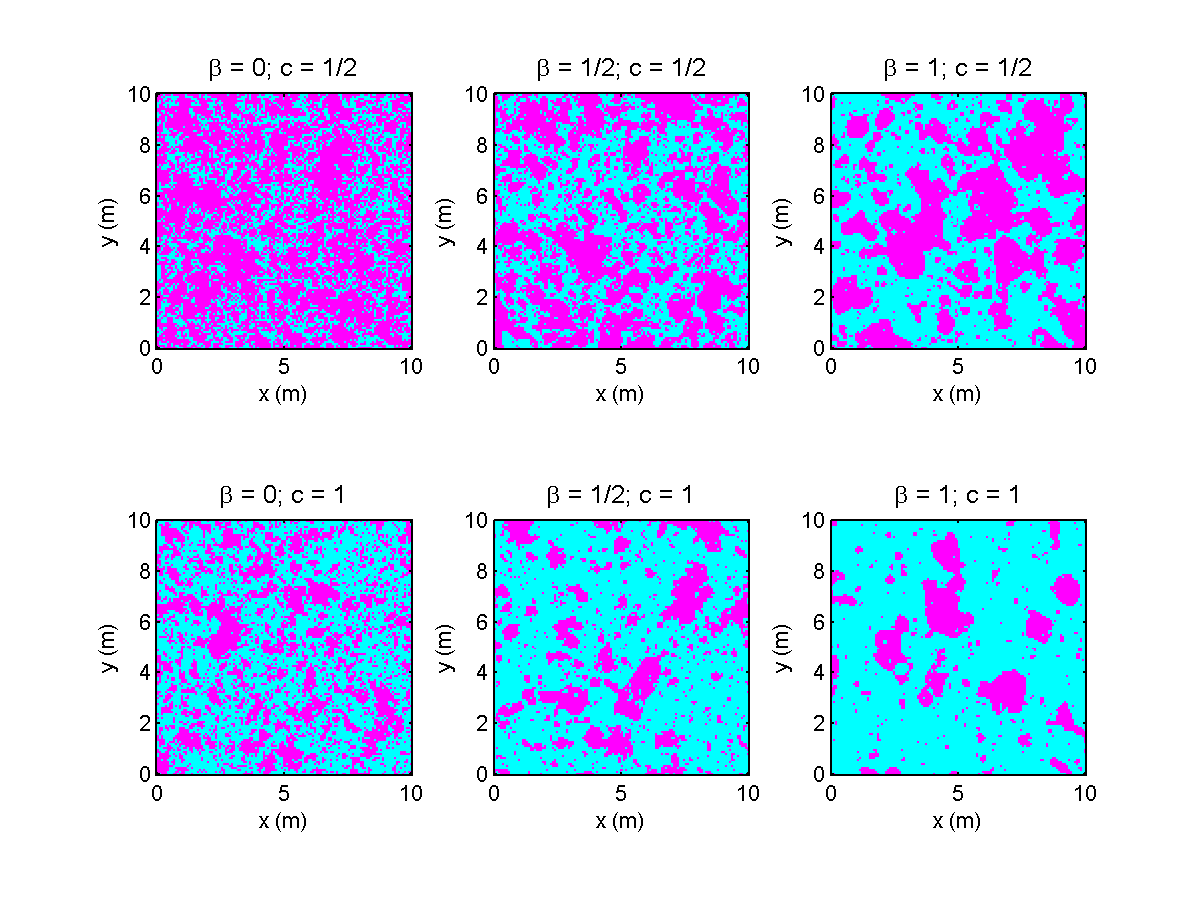
Figure 24 shows example realizations of two-phase media, as calculated by the double-sided level-cut method described in Sec. 3.5. As the parameter $\beta$ is increased, the number of small objects decreases. For a given value of $\beta$, larger values of the level cut increase the void fraction.

As mentioned earlier, the preceding modeling approach leads to mutually independent QW positions; that is, realizations with no spatial organization. This is analogous to the basic cratering process described in Sec. 2.2. However, the fractal support techniques described in Sec. 2.3 could also be used to modulate the Poisson process for QW placements, and thus organize the QWs into active regions.

In Sec. 2.3, it was shown that a cratering process with a packing fraction of $\phi^{\prime}$ for the support leads to a packing fraction for size class $i$ of $\phi_{i}\approx\phi(1-\phi^{\prime})^{i-1}$, where $\phi$ is the “full activity” level for the packing fraction, which applies to the initial size class. Comparing to Eq. 17, we see that the desired packing fractions of the individual classes can be obtained by setting $\overline{\phi}=1-\phi^{\prime}$ and $\phi_{1}=\phi$. This simple prescription allows a spatially organized QW model with decreasing packing fraction ($\overline{\phi}<1$, or equivalently $\beta>0$) to be simulated from a cratering process for the fractal support, with a constant packing fraction $\phi^{\prime}=1-\overline{\phi}$, which modulates a QW model, with a constant packing fraction $\phi=\phi_{1}$.

Example realizations of processes without and with spatial organization (i.e., homogeneous and fractal supports, respectively) are shown in Fig. 25. Both realizations are for $\beta=\lambda=1/4$. (These values of $\beta$ and $\lambda$ satisfy the constraint for turbulence, to be derived in Sec. 4.3.) The fractal support causes the smaller QWs to be concentrated in certain regions; other regions have a relatively smooth, inactive appearance. This behavior is reminiscent of many of the example RHM shown in the Introduction, such as the simulations of turbulence (Fig. 5).

Let us consider constraints between the scaling parameters pertinent to the modeling of turbulence. For turbulent velocity fluctuations, the amplitudes $q_{i}$ may be identified as the turbulent velocities associated with the QWs, $\upsilon_{i}$. According to Kolmogorov’s (1941) hypothesis, the transfer rate of specific turbulent kinetic energy (TKE) from one scale to the next is invariant, and equal to the dissipation at the molecular scale, $\epsilon$. Let us define $\Delta\Lambda_{i}$ as the net transfer rate of energy (the flux) from scale $i$ to $i+1$. This quantity has dimensions of (length)² (time)^-3. By dimensional analysis, one has

$$\Delta\Lambda_{i}=\epsilon\propto\phi_{i}\frac{\upsilon_{i}^{3}}{a_{i}}.$$

(27)

The factor $\phi_{i}$ adjusts for the volume occupied by the QWs, so that $\Delta\Lambda_{i}$ represents the transfer specific to the active volume. Setting $\Delta\Lambda_{i}=\Delta\Lambda_{i+1}$, we find

$$\overline{q}=\ell^{1/3}\overline{\phi}^{(-1/3)}=\ell^{(1-\beta)/3}.$$

(28)

Comparing to Eq. 21, we have the following constraint for turbulence:

$$\lambda=(1-\beta)/3.$$

(29)

Later, in Sec. 6, we will see that this constraint is consistent with Kolmogorov’s well known “$-11/3$ law” for the spectrum.

Consider now a cascade process which transfers energy from large QWs to smaller ones, as well as vice versa. The former process is termed decay or forward scatter, whereas the latter process is termed backscatter (Kim et al.,, 2008). Let us define $\Lambda_{i\rightarrow j}$ as the energy flux from generation (size class) $i$ to $j$. (In this section, it will be assumed that there is no scale densification, i.e., the size classes are integers.) A steady-state model must balance the energy being transferred into the size class with that going out. Assuming that transfers occur only between adjacent size classes, the following equation describes the flux balance for class $i$:

$$\Lambda_{i\rightarrow i-1}+\Lambda_{i\rightarrow i+1}=\Lambda_{i-1\rightarrow i}+\Lambda_{i+1\rightarrow i}+S_{i}.$$

(53)

The terms on the left side, $\Lambda_{i\rightarrow}\equiv\Lambda_{i\rightarrow i-1}+\Lambda_{i\rightarrow i+1}$, represent transfer from class $i$ to larger and smaller scales (back and forward scatter), respectively. The terms on the right, $\Lambda_{\rightarrow i}\equiv\Lambda_{i-1\rightarrow i}+\Lambda_{i+1\rightarrow i}$, represent transfer to class $i$ from larger and smaller scales (forward and back scatter), respectively. Also present is a source term $S_{i}$, which represents the creation of QWs of size $a_{i}$ by an external process. This situation is depicted graphically in Fig. 28. The previous one-way cascade model corresponds to a per-volume energy production rate at the largest scale of $S_{1}=\mathcal{N}_{1}E_{1}/\tau_{1}=\mathcal{R}_{1}E_{1}$, whereas $S_{i}=0$ for $i\neq 1$. The backscatter terms, $\Lambda_{i\rightarrow i-1}$, are all zero.

Of particular interest is the net energy transfer between two adjacent size classes. The net transfer from class $i$ to $i+1$ is

$$\Delta\Lambda_{i}=\Lambda_{i\rightarrow i+1}-\Lambda_{i+1\rightarrow i}.$$

(54)

From Eq. 53, we have

$$\Delta\Lambda_{i}=\Delta\Lambda_{i-1}+S_{i}.$$

(55)

Since it is assumed there is no transfer from unresolved scales, we define $\Delta\Lambda_{0}=-\Lambda_{1\rightarrow 0}$ and $\Delta\Lambda_{N}=\Lambda_{N\rightarrow N+1}$. In the absence of a source, the net transfers to and from each size class must balance. Consider the situation when there is the only non-zero source term, for $i=j$. Then $\Delta\Lambda_{j}=\Delta\Lambda_{j-1}+S_{j}$, $\Delta\Lambda_{0}=\Delta\Lambda_{1}=\cdots=\Delta\Lambda_{j-1}$, and $\Delta\Lambda_{N}=\Delta\Lambda_{N-1}=\cdots=\Delta\Lambda_{j}$. The case $j=1$ corresponds to Kolmogorov’s hypothesis; that is, all of the $\Delta\Lambda_{i}$ must equal the source term $S_{1}$.

Let us now assume that a certain fraction $f$ of the total energy transferred into the size class is always subsequently transferred to smaller scales, i.e., forward scattered. Such an assumption implies that the energy cascade is scale invariant. Notationally,

$$\Lambda_{i\rightarrow i+1}=f\left(\Lambda_{\rightarrow i}+S_{i}\right),\ i=1,\cdots,N.$$

(56)

The remaining fraction, $1-f$, is transferred to larger scales (the backscatter).

$$\Lambda_{i\rightarrow i-1}=(1-f)\left(\Lambda_{\rightarrow i}+S_{i}\right),\ i=1,\cdots,N.$$

(57)

Note that Eq. 53 is recovered when Eq. 56 is added to Eq. 57. Eqs. 56 and 57 together provide a system of $2N$ linear equations that can be solved by standard matrix techniques. (The fluxes $\Lambda_{0\rightarrow 1}$ and $\Lambda_{N+1\rightarrow N}$ are set to 0.)

References

- Anderson et al., (2004) Anderson, T. S., Moran, M. L., Ketcham, S. A., and Lacombe, J. (2004). Tracked vehicle simulations and seismic wavefield synthesis in seismic sensor systems. Comput. Sci. Eng., 6(6):22–28.
- Bendat and Piersol, (2011) Bendat, J. S. and Piersol, A. G. (2011). Random Data: Analysis and Measurement Procedures. John Wiley & Sons, New York.
- Field and Grigoriu, (2012) Field, R. V. and Grigoriu, M. (2012). Level cut gaussian random field models for transitions from laminar to turbulent flow. Probabilist. Eng. Mech., 28:91–102.
- Frisch et al., (1978) Frisch, U., Sulem, P.-L., and Nelkin, M. (1978). A simple dynamical model of intermittent fully developed turbulence. J. Fluid Mech., 87(4):719–736.
- Goedecke et al., (2004) Goedecke, G. H., Ostashev, V. E., Wilson, D. K., and Auvermann, H. J. (2004). Quasi-wavelet model of von Kármán spectrum of turbulent velocity fluctuations. Bound.-Lay. Meteorol., 112(1):33–56.
- Goedecke et al., (2006) Goedecke, G. H., Wilson, D. K., and Ostashev, V. E. (2006). Quasi-wavelet models of turbulent temperature fluctuations. Bound.-Lay. Meteorol., 120(1):1–23.
- Grigoriu, (2003) Grigoriu, M. (2003). Random field models for two-phase microstructures. J. Appl. Phys., 94(6):3762–3770.
- Gurvich and Kukharets, (1986) Gurvich, A. S. and Kukharets, V. P. (1986). The influence of intermittence of atmopsheric turbulence on the scattering of radio waves. Sov. J. Commun. Technol. Electron., 30:52–58. English transl.
- Hentschel and Procaccia, (1983) Hentschel, H. G. E. and Procaccia, I. (1983). Passive scalar fluctuations in intermittent turbulence with applications to wave propagation. Phys. Rev. A, 28:417–426.
- Kim et al., (2008) Kim, T., Thürey, N., James, D., and Gross, M. (2008). Wavelet turbulence for fluid simulation. In ACM Transactions on Graphics (TOG), volume 27, page 50. ACM.
- Kolmogorov, (1941) Kolmogorov, A. N. (1941). The local structure of turbulence in incompressible viscous fluid for very large Reynolds numbers. In Dokl. Akad. Nauk SSSR, volume 30, pages 299–303.
- Kolmogorov, (1962) Kolmogorov, A. N. (1962). A refinement of previous hypotheses concerning the local structure of turbulence in a viscous incompressible fluid at high Reynolds number. J. Fluid Mech., 13(1):82–85.
- Lapin, (1980) Lapin, L. L. (1980). Statistics: Meaning and Method. Harcourt Brace Jovanovic, New York.
- Mahrt, (1989) Mahrt, L. (1989). Intermittency of atmospheric turbulence. J. Atmos. Sci., 46(1):79–95.
- Mandelbrot, (1974) Mandelbrot, B. B. (1974). Intermittent turbulence in self-similar cascades: divergence of high moments and dimension of the carrier. J. Fluid Mech., 62(2):331–358.
- Mandelbrot, (1977) Mandelbrot, B. B. (1977). Fractals: Form, Chance, and Dimension. W.H. Freeman, San Francisco.
- Obukhov, (1962) Obukhov, A. M. (1962). Some specific features of atmospheric turbulence. J. Geophys. Res., 67(8):3011–3014.
- Ostashev, (1997) Ostashev, V. E. (1997). Acoustics in Moving Inhomogeneous Media. E & FN Spon, London.
- Rytov et al., (1989) Rytov, S. M., Kravtzov, Y. A., and Tatarskii, V. I. (1989). Principles of Statistical Radio Physics, Part 4: Wave Propagation through Random Media. Springer, Berlin.
- Schroeder, (1991) Schroeder, M. (1991). Fractals, Chaos, Power Laws. W.H. Freeman, San Francisco.
- Sreenivasan, (1991) Sreenivasan, K. R. (1991). Fractals and multifractals in fluid turbulence. Annu. Rev. Fluid Mech., 23(1):539–604.
- Tatarskii, (1971) Tatarskii, V. I. (1971). The Effects of the Turbulent Atmosphere on Wave Propagation. Keter, Jerusalem.
- Tatarskii and Zavorotnyi, (1985) Tatarskii, V. I. and Zavorotnyi, V. U. (1985). Wave propagation in random media with fluctuating turbulent parameters. J. Opt. Soc. Am. A, 2:2069–2076.
- Torrence and Compo, (1998) Torrence, C. and Compo, G. P. (1998). A practical guide to wavelet analysis. B. Am. Meteorol. Soc., 79(1):61–78.
- (25) Wilson, D. K., Lawson, D. E., Albert, D. G., Bigl, M. F., Finnegan, D., Ostashev, V. E., and Goedecke, G. H. (2008a). Wave scattering and sensing strategies in intermitent terrestrial environments. In 26th Army Science Conference, Orlando, FL.
- Wilson et al., (2005) Wilson, D. K., Moran, M. L., Ketcham, S. A., Lacombe, J., Anderson, T. S., Symons, N. P., Aldridge, D. F., Marlin, D. H., Collier, S. L., and Ostashev, V. E. (2005). High-fidelity simulation capability for virtual testing of seismic and acoustic sensors. In Proc. SPIE, volume 5796, pages 105–116.
- (27) Wilson, D. K., Ostashev, V. E., and Goedecke, G. H. (2008b). Sound-wave coherence in atmospheric turbulence with intrinsic and global intermittency. J. Acoust. Soc. Am., 124:743–757.
- Wilson et al., (2009) Wilson, D. K., Ostashev, V. E., and Goedecke, G. H. (2009). Quasi-wavelet formulations of turbulence and other random fields with correlated properties. Probabilist. Eng. Mech., 24(3):343–357.
- Wilson et al., (1996) Wilson, D. K., Wyngaard, J. C., and Havelock, D. I. (1996). The effect of turbulent intermittency on scattering into an acoustic shadow zone. J. Acoust. Soc. Am., 99:3393–3340.