Pinning of thermal excitations at defects in artificial spin-ice dipolar arrays:
A theoretical investigation

Topologically frustrated systems offer unexpected properties which have been studied recently in magnetic materials. A particular exciting system is artificial spin ice with its ‘exotic’ magnetic ground state [1, 2, 3, 4]. Artificial spin ice is a two-dimensional (2D) array of magnetic nanoislands fabricated with desired geometries. The nanoislands are typically elongated to show a single-domain state; their magnetic moments then point in one of two directions. Being isolated from each other, e. g., separated by a distance in the order of several hundred nanometer, they are coupled by the long-range dipole-dipole interaction.

The systems sketched above are known for low-temperature fractionalization: they exhibit collective excitations that carry only a fraction of the elementary constituent’s properties. These appear due to the absence of a unique ground state and due to the violation of the ‘two-in-two-out’ ice rule, the latter proposed by Pauling for the proton ordering in water ice [5]. Collective excitations appear as ferromagnetically aligned nanoislands (‘strings’) with end points (‘nodes’ or ‘vortices’) that behave like magnetic charges, known as Nambu magnetic monopoles [6, 7, 8, 9, 10]. The oppositely charged end nodes of the strings interact with each other with a distance dependence of a Coulomb potential [8]. The properties of these artificial magnetic monopoles are studied theoretically as well as experimentally with great effort. We recall that magnetic monopoles would ‘symmetrize’ electrodynamics with respect to the electric and the magnetic field [11, 12].

Improvements in nanolithography allow to design artificial spin ice in 2D structures like honeycomb (kagomé ice) [13, 14, 10, 15], brickwork [16, 17], triangular [18], and pentagonal [19] lattices. A three-dimensional artificial spin ice can be realized, e. g., by a layer-by-layer synthesis [19]. Local modifications in the otherwise perfect array are introduced by local nanolithography [20, 21]. These perturbations, considered as defects, modify significantly the properties of the system [22, 23]. This leads to a question on the role of defects in dipolar arrays concerning thermal excitations. For three-dimensional spin ice and pyrochlore lattices, defects have already been studied by Jaubert [24]. First investigations of defects in 2D artificial spin ice have been performed by Silva et al. [25] who investigated the interaction between magnetic string excitations caused by defects and Nambu string excitations. Since defects can serve as pinning centers in magnetic materials[26, 27], it is conceivable to influence and control magnetic monopoles and the associated string excitations by tailoring the defects’ properties.

Experimentally, effective thermal excitations in artificial square dipolar arrays can for example be provided by field protocols[28, 29] of vibro-fluidized granular matter, allowing investigations of the short-range magnetic order. Long-range ordered ground states in square-lattice spin ice were obtained by thermal annealing during the fabrication [9], which is recommended for magnetic monopoles of charges $\pm 2$. Charges of $\pm 4$ were not observed, which is attributed to the nanoislands’ geometry. Recent investigations on artificial spin ice with reduced nanoislands’ dimension [30] proved thermal excitations at room temperature, which allows not only to observe but also to control excitations with large magnetic charges.

In this work, we study various defect types in square-lattice artificial spin ice, with a focus on magnetic excitations. We consider modifications of two nanoislands of a vortex as a defect: (i) removal of two islands from the vortex, (ii) a vertical displacement of two islands, (iii) a modification of the islands’ thickness or (iv) of their magnetization density. Furthermore, two defects with predefined positions and properties have been introduced into the spin ice. The resulting string excitations that link these defects are analyzed with respect to defect position and string length. Magnetic ground states have been achieved by Monte Carlo simulations for given temperatures [31, 32].

The paper is organized as follows. Theoretical aspects are presented in Section II. In the discussion of the results, given in Section III, we address randomly distributed vacancies (III.1) before analyzing one or two defects with prescribed properties (III.2). We conclude with Section IV.

We build up the artificial spin ice by nanomagnets whose dimension has been taken from Ref. 30 (length $470\,\mathrm{nm}$, width $170\,\mathrm{nm}$, and height $3\,\mathrm{nm}$). The lattice constant $a$ of the square lattice [33] is $793.8\,\mathrm{nm}$ (the lattice spacing in Ref. 34 is $425\,\mathrm{nm}$). The magnetic single-domain state of each elongated nanoisland is described by a magnetization vector $\pm\bm{M}$ (‘spin’) aligned along the large island axis. For islands made of permalloy, $|\bm{M}|\approx 200\cdot 10^{3}\,\mathrm{Am^{-1}}$.

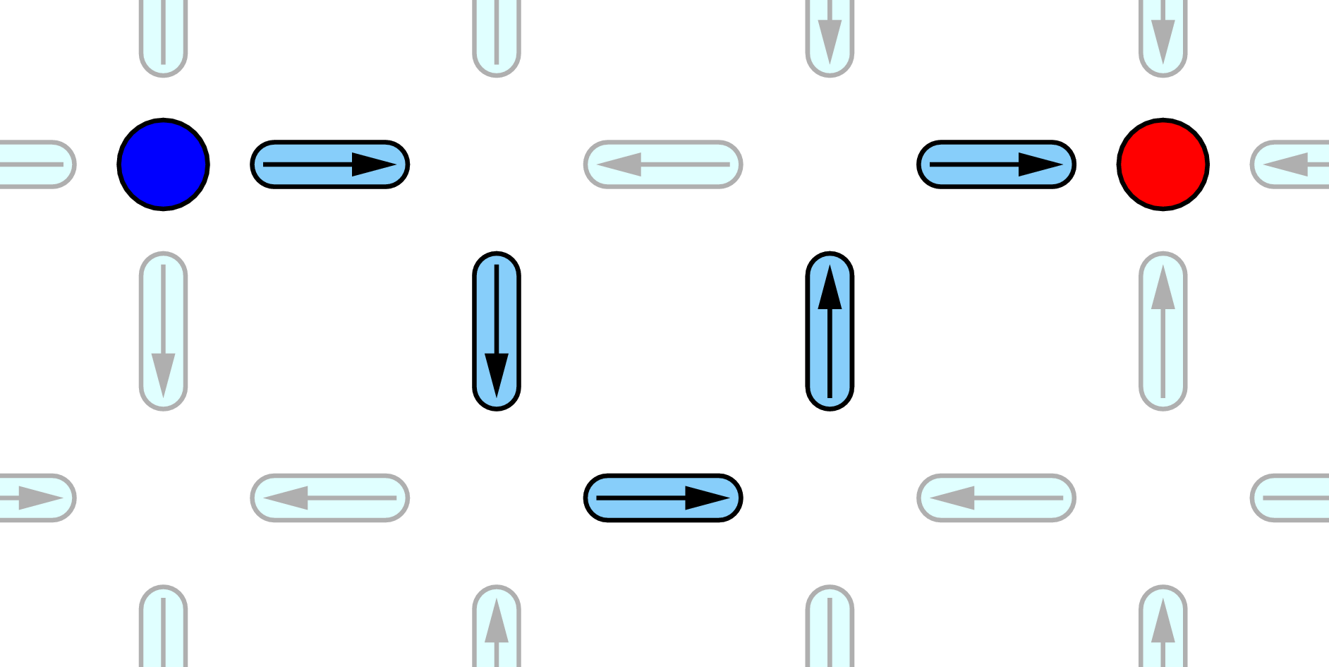
Four islands that form a cross introduce a node (‘vortex’; cf. Fig. 1a). The number of spins pointing toward the node’s center $\bm{C}$ define the charge $Q$ of that node ($Q\in\{-4,-2,0,+2,+4\}$; for example, $Q=0$ in Fig. 1a). To quantify thermal activation, we introduce the fraction of nodes with charge $Q$ in the sample, $\eta_{Q}\equiv N_{Q}/N$ ($N$ number of nodes with four adjacent islands in the sample); on average $\langle\eta_{Q}\rangle=\langle\eta_{-Q}\rangle$. A path of ferromagnetically aligned nanoislands that connects a pair of nodes with opposite non-zero charges is called a ‘string excitation’ (Fig. 2).

Instead approximating the nanomagnets as points[35, 7, 8] or dipolar needles[35, 10], we compute the dipole-dipole interaction energies for realistic shapes. This is done numerically, allowing in principle for arbitrarily shaped nanoislands. It turns out that the dipolar interaction[36, 37] is relevant only for first- (1NN) and for second-nearest (2NN) neighbors,[38, 39] with energies $E_{\mathrm{1NN}}$ and $E_{\mathrm{2NN}}$, respectively.

The interaction energies $E_{\mathrm{1NN}}$ and $E_{\mathrm{2NN}}$ can be modified in various ways: by (i) introducing vacancies (i. e., removal of two islands from a node), (ii) modifying an island’s magnetization density (Fig. 1a), (iii) varying the vertical displacement $\delta z$ (Fig. 1b), and (iv) increasing an island’s thickness (Fig. 1c). These modifications keep the charges $Q$ even. Local modifications of the free-energy landscape are achieved by introducing defects into the dipolar arrays.

To obtain a magnetic ground state, we use Monte Carlo simulations based on the Metropolis algorithm [31, 32]. The energy barrier $\Delta E$ between the two possible magnetization states $\pm\bm{M}$ of the nanoislands is considered. A slight reduction of the temperature in each step drives the system toward a free-energy minimum by successively reversing the islands’ spins. A typical Monte Carlo simulation comprises at least 100 000 steps. In this Paper, we report on results for lattices with $20\times 20$ cells and with $50\times 50$ cells, each with $2$ nanomagnets ($N_{\mathrm{spin}}=20\times 20\times 2=800$ or $5000$). These samples are large enough to suppress even minute finite-size effects, as has been checked by comparison with calculations for larger arrays.

The magnetic ground state of artificial spin ice at small finite temperature ($T\approx 1\,\mathrm{K}$) is dictated by the (spin) ice rule: at a node with center $\bm{C}$, two spins pointing inward and two spins pointing outward (‘2In2Out’ rule, $Q=0$). Hence, $\eta_{0}=100\,\mathrm{\%}$. Determined by the interaction energies $E_{\mathrm{1NN}}$ and $E_{\mathrm{2NN}}$, the ground state is ‘2in2outOp’ for $\delta_{z}=0$, in agreement with earlier work (e. g., Ref. 8); it shows inward pointing spins at opposite (‘Op’) nanomagnets. This state shows a degree of degeneracy of $2$, with the energy $E=\left(-4E_{\mathrm{1NN}}+2E_{\mathrm{2NN}}\right)N_{\mathrm{spin}}$ ($N_{\mathrm{spin}}$ number of spins in the sample). The configuration ‘2In2OutAd’ has an energy of $-2E_{\mathrm{2NN}}N_{\mathrm{spin}}$, is four-fold degenerate, and consists of inward pointing spins at adjacent (‘Ad’) islands [39].

The ‘2In2OutOp’ configuration imposes a vortex structure described by a $c(2\times 2)$ magnetic unit cell (cf. the checkerboard structure on the left-hand side of Fig. 3). While for ‘2In2OutOp’ a vortex chirality can be ascribed to each plaquette, this is not the case for the ‘2In2OutAd’ configuration. Consequently, the latter displays a $p(2\times 2)$ magnetic unit cell (on the right-hand side of Fig. 3).

By displacing vertically the rows and columns of the square lattice, the degeneracies of the above configurations can be tuned to $6$ for a critical $\delta z_{\mathrm{c}}$ (Ref. 39), that is, to the same degree of degeneracy as in water ice[5], in pyrochlore lattices[40, 41], and in kagomé lattices[42] (In the honeycomb and square lattice this sixfold degeneracy is out of 8 and 16 possible vertices, respectively. However, one may consider both lattices and their magnetic ground states equivalent because both have the same residual entropy of $0.2\,k_{\mathrm{B}}$; cf. Ref. 39). Consequently, a transition from $c(2\times 2)$ to $p(2\times 2)$ ordering takes place at this critical displacement. For $\delta z<\delta z_{\mathrm{c}}$, ‘2in2outOp’ nodes prevail, while for $\delta z>\delta z_{\mathrm{c}}$, ‘2in2outAd’ vortices prevail. The critical value $\delta z_{\mathrm{c}}$ depends on the islands’ shape: $\delta z=0.27\,a$ for the realistic shapes used in this investigation (cf. Ref. 39), $0.418\,a$ in Ref. 35, and $0.444\,a$ in Ref. 8.

In what follows, we distinguish two types of arrays: $\mathcal{S}_{1}$ has $\delta_{z}=0$, a vanishing residual (zero-temperature) entropy and exhibits the ‘2In2OutOp’ ground state. In contrast, $\mathcal{S}_{2}$ has the critical $\delta_{z}=0.27\,a$, shows a residual, finite entropy of $S=0.2\,k_{\mathrm{B}}$ (Ref. 43) and its ground state is comprised of ‘2In2OutOp’ and ‘2In2OutAd’ vortices. The temperature is $T=300\,\mathrm{K}$ (room temperature).

In this theoretical investigations we have shown that thermal string excitations can be pinned at modified nanomagnets in a dipolar array. The different types of defects may be produced by microstructuring techniques. It turned out that a decrease of the islands’ magnetization density is most efficient in creating nodes with large charges. On top of this, a pair of defects is connected by a ferromagnetic path of islands, that is, by a string excitation.

The length of the pinned strings is closely related to magnetic ground state configuration and to the position of the defects. This finding suggests experimental and theoretical investigations of topology and formation of magnetic domains.