Gaussian linear state-space model for wind fields in the North-East Atlantic

The observed wind fields are generally smooth leading to a high correlation between the different sites. It suggests that it may be possible to explain an important part of the signal by using a common scalar process (the regional wind condition) for the different locations. This scalar process, denoted $\{X_{t}\}$ in the sequel, is not directly observable and is introduced as a latent process. Due to the mean motion of air masses we expect that the wind conditions at western locations will depend more on the leading one lag $X_{t+1}$ and $X_{t}$ signals than on the lagged signal $X_{t-1}$ with the reverse phenomenon at eastern locations. These points led us to consider the following Gaussian state-space model

$Y_{t}\in\mathbb{R}^{K}$ is the observed process, its $K$ coordinates correspond to the mean corrected transformed wind speed at the $K=18$ locations. $\{\epsilon_{t}\}$ and $\{\eta_{t}\}$ are independent Gaussian white noise sequences with zero means and identity covariance matrices. $\alpha_{1}$, $\alpha_{0}$ and $\alpha_{-1}$ are $K$-dimensional vectors which link the lagged values of the regional process $\{X_{t}\}$ to local wind conditions. The covariance matrix $\Gamma\in\mathbb{R}^{K\times K}$ models the spatial structure of the difference between the observed process $\{Y_{t}\}$ and the local conditions $W_{t}=\alpha_{1}X_{t+1}+\alpha_{0}X_{t}+\alpha_{-1}X_{t-1}$ deduced from the regional process. It may correspond to small scale fluctuations. In finance and economics this covariance matrix of error of measurement is often diagonal. In [WH10] a parametrization of this matrix or the use of a diagonal matrix are advised. As a first step this covariance matrix is not parameterized but reduced models which take into account the spatial information are investigated in Subsection 5.1. In the sequel we denote $\Lambda=(\alpha_{1}|\alpha_{0}|\alpha_{-1})\in\mathbb{R}^{K\times 3}$ and $\theta=\left(\rho,\sigma,\Lambda,\Gamma\right)$ the unknown parameter.

The temporal dynamics of the observed process is mainly contained in the latent process $\{X_{t}\}$. The model thus imposes the same long term temporal dynamics, corresponding to the regional scale, at each location. Under the assumption $\mathinner{\!\left\lvert\rho\right\rvert}<1$, the AR(1) process $\{X_{t}\}$ is stationary and so is the process $\{Y_{t}\}$. $\{W_{t}\}$ is an ARMA(1,2) process since

Signs and values of $(\alpha_{1},\alpha_{0},\alpha_{-1})$ can be interpreted in terms of autocovariance function of the moving average part $\alpha_{1}\epsilon_{t+1}+\alpha_{0}\epsilon_{t}+\alpha_{-1}\epsilon_{t-1}$.

Identifiability is required to get sensible and reliable parameter estimation. Gaussian linear state-space models are often non-identifiable without additional constraints (see e.g. [HD88], [Lju99], [BW12], [Bor10]). Indeed the introduction of the latent process $\{X_{t}\}$ is a source of non-identifiability since the unknown parameters need to be identified uniquely from the distribution of the observed $\{Y_{t}\}$.

$\{Y_{t}\}$ is a zero mean stationary Gaussian process which is thus characterized by its second order structure given below

The study of this space-time covariance function leads to the following Proposition which is proven in Appendix A.

These identifiability constraints were always satisfied when fitting the model to the data. The first condition requires $X$ to have a unit stationary variance, the local variability is then accounted in the vectors $\alpha_{1}$, $\alpha_{0}$ and $\alpha_{-1}$. The second one is natural since in case of linear dependence between these vectors the model (M) is reduced to a sub-model dealing with one or two lagged versions of $X$. Identifiability of linear Gaussian state-space models have been investigated during the last decades and initially in control theory. Literature is abundant on stochastic linear systems identification ([Lju99, HD88]). To the best of our knowledge most of sufficient conditions of identifiability are structural constraints on parameters (see [PD10] for references and examples) associated with identification procedures. Identifiability is examined through different criteria such that transfer functions ([Lju99]) or likelihood criterion like in [PD10]. Identification procedures are realized through controllability and observability of several parameters in [Lju99] and via the EM algorithm in [PD10]. In econometrics the identifiability of the latent factors and the loading matrix is considered (see for example [BW12, Bor10]). In most cases structural constraints are also applied depending on the interpretability desired. However the general conditions given in [BW12] do not guarantee identifiability of the model (M) since $X$ is scalar in (M).

Considering the function defined by (1-3) as a discretized space-time covariance function, we show in Appendix A that properties of full-symmetry and separability are not fulfilled under the identifiability constraints of Proposition 1. Other non-symmetric space-time covariance models have been proposed in the literature and some of them have been adjusted to the Irish wind dataset that exhibits non-symmetry (see [Gne02] and [FHI07, chapter 4]). Strong spatial assumptions are commonly assumed in these models such as spatial stationarity and isotropy. However due to prevailing flows a lot of meteorological data have anisotropic patterns like the dataset under study or the Irish one. A model, based on the specification of a vector autoregressive process, is proposed in [dLG05] to capture a part of the anisotropy that is observable in the correlations of the Irish dataset. We will see in Section 4 that the proposed model enables to reproduce various above mentioned complex properties of the space-time covariance of our wind data.

Two methods of estimation have been implemented and compared. The first one is a method of moment based on the second order structure of the process $\{Y_{t}\}$ given by (1-3). It consists in minimizing numerically the following objective function

where $\widehat{\mathrm{cov}}$ denotes the empirical covariance function and $\|.\|_{2}$ stands for the matrix Frobenius norm. This method, denoted GMM in the sequel, is a standard method in geostatistics (see e.g. [Cre91]). We have chosen to consider only the first four lags of the autocovariance function when building the objective function (4). It corresponds to the minimal number of terms needed to identify the parameters (see Appendix A). Simulation results indicate that including more lags in the objective function does not lead to more accurate estimates.

The second method performs Maximum Likelihood (ML) estimation using the Expectation-Maximization (EM) algorithm ([CMR05] and [DLR77]). For linear Gaussian state-space model efficient numerical procedures exist for both the E-step, where the Kalman recursions lead to an exact computation of the smoothing probabilities, and the M-step with analytical expressions being available for the parameters which maximize the intermediate function of the EM algorithm. More details can be found in the supplementary materials.

Both methods are sensitive to the initial parameter value which needs to be chosen carefully. We used the following procedure which exploits the properties of the second order structure of $\{Y_{t}\}$:

• -

  $\rho=\displaystyle\frac{\mathrm{cov}(Y_{t},Y_{t+3})_{i,j}}{\mathrm{cov}(Y_{t},Y_{t+2})_{i,j}}$ for all $i,j\in\{1,...,K\}$ is initialized as the empirical mean of $\displaystyle\frac{\widehat{\mathrm{cov}}(Y_{t},Y_{t+3})_{i,j}}{\widehat{\mathrm{cov}}(Y_{t},Y_{t+2})_{i,j}}$.

• -

  $\Lambda$ is estimated by minimizing

  $\displaystyle\theta_{\Lambda}$

  $\displaystyle\rightarrow$

  $\displaystyle\|\widehat{\mathrm{cov}}(Y_{t},Y_{t+1})-\mathrm{cov}_{\theta}(Y_{t},Y_{t+1})\|_{2}^{2}+\|\widehat{\mathrm{cov}}(Y_{t},Y_{t+2})-\mathrm{cov}_{\theta}(Y_{t},Y_{t+2})\|_{2}^{2}$

  as a function of $\Lambda$ with $\rho$ being fixed to the value obtained in the previous step. Note that this function does not depend on $\Gamma$ according to (2) and (3).

• -

  $\Gamma$ is determined by minimizing

  $\displaystyle\theta_{\Gamma}$

  $\displaystyle\rightarrow$

  $\displaystyle\|\widehat{\mathrm{cov}}(Y_{t},Y_{t})-\mathrm{cov}_{\theta}(Y_{t},Y_{t})\|_{2}^{2}$

  as a function of $\Gamma$ with $\rho$ and $\Lambda$ being fixed to the value obtained in the previous steps.

These rough estimates are used as initial conditions for the numerical optimization of 4 which leads to the GMM estimates. The GMM estimates are then used to initialize the EM algorithm and get the ML estimates.

Under suitable conditions, GMM (see [NM94]) and ML (see [NM94, SS06, HD88, Cai88]) estimators are consistent and asymptotically Gaussian. A simulation study was performed in order to assess the performance of the estimates in a situation comparable to the practical application. $N=100$ independent sets of the size of the studied data are simulated for the parameters set estimated by ML on the wind data. Table 1 gives the bias, standard deviation and Root Mean Square Error (RMSE) of ML and GMM estimates computed from the simulations. Bias and standard deviations are low. ML generally outperforms GMM except for estimating $\Gamma$ where both methods give comparable results. For both methods $\alpha_{1}$ and $\alpha_{-1}$ are more accurately estimated than $\alpha_{0}$ and $\Gamma$ is the less accurately estimated quantity.

The loading matrix $\Lambda$ links the latent process to observed wind conditions. The values of $\alpha_{1}$ and $\alpha_{-1}$ shown on Figure 3 reveal the site-dependent relations with the regional mean wind. As expected western locations, which are generally the first affected when meteorological events enter in the studied region, depend more on $X_{t+1}$ than on $X_{t-1}$ and the reverse is true for eastern locations.

Since large scale variability is supposed to be contained in the latent process, $\Gamma$ should contain only small scale variations due to the differences between the observed wind $\{Y_{t}\}$ and the downscaled regional wind $\{W_{t}\}$. This is confirmed when comparing the spatial sill and range of $\Gamma$ with the ones of the original covariance function of the data (see Figure 4). The shape of $\Gamma$ has a block structure which is induced by the geometry of the domain and the numbering of the sites (see Figure 1). The level sets of the blocks, except the top right corner (and by symmetry bottom left corner), are similar to saddle point level sets: the model better explains the wind observed at the central locations of the domain than at the locations which are close to the boundary. The top right corner has elliptical level sets. This different geometry raises problems when trying to develop simple parametric model for $\Gamma$ (see Section 5.1).

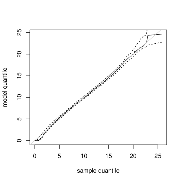
To further validate the model we have checked its ability to simulate realistic wind conditions. For that we have generated artificial time series from the model, and have compared statistics corresponding to the artificial sequences with those from the original data. We first looked at the marginal distributions of wind speed, both observed and fitted, at each location. According to quantile-quantile plots shown on Figure 5, the model is able to reproduce the general shape of the marginal distribution of the process at the central station $9$ except for very low wind speed. Similar results were obtained at other locations.

The model assumes that the dynamics of wind speed are inherited mainly from the common latent process $\{X_{t}\}$. To check this assumption, we have compared the autocorrelation functions of the model to the data ones at the various locations. Typical results are shown in Figure 6. The model is able to reproduce the first coefficients of the autocorrelation function at the central location $9$ and of the cross-correlation function between locations $13$ and $18$ which exhibits a time shift due to the prevailing westerly flow. GMM estimate is designed to make coincide the first lags of the empirical autocovariance functions with the one of the fitted model. Figure 6 shows that the agreement is indeed very good. However the ML method, which takes into account the longer term dynamics in the likelihood function, is better in reproducing the correlation structure for time lags above one day. It is mainly due to the higher value of $\rho$ ($0.76$ by ML and $0.70$ obtained by GMM). The better performance of ML estimates is coherent with Table 1. Figure 6 also shows the important bias on the estimates of the second order structure of the process which is problematic when using the GMM approach.

Figure 7 shows the theoretical correlations at lags $0$ and $1$ against the empirical ones to assess the model’s ability to capture the spatial dependence structure. Correlations at lag 0 are very well reproduced and lagged one correlations are also generally well reproduced. As expected, the GMM method provides again a better fit. Similar figures than Figure 2 reveal that the anisotropy and non-separability observable in the correlations are partly reproduced by the model.

An advantage brought by the Markovian structure of the model ($\mathrm{M}$) is that short term forecast can be efficiently computed through the Kalman recursions (see [BD06, chapter 8]). The forecast performance is assessed by computing the one-step ahead forecast on the last $8$ years of data (validation set) after fitting the model on the first $25$ years of data (training set). In practice the forecast skill of the model at location $i\in\{1,...,K\}$ is evaluated by computing the natural empirical estimate of the Mean Square Percentage Error (MSPE) defined as

where the MSE of the forecast error (the numerator) is normalized by the variance of the field at the individual locations, with $Y_{t}$ the original non transformed wind.

According to Table 2, model ($\mathrm{M}$) leads to significant improvements over persistence forecast (about 28%), which is the classical benchmark for wind prediction (see e.g. [ZG12]), and the forecast obtained when fitting a different ARMA(2,1) model at each site (about 17%). It illustrates the gain of using the spatial information when computing short-term probabilistic forecasts. For comparison purpose, a vector autoregressive model of order $1$ (VAR(1)) was also fitted. The VAR(1) model gives slightly better results compared to model ($\mathrm{M}$) with an improvement of about $9\%$ in average over all locations. However the VAR(1) model involves $495$ parameters, compared to the $208$ parameters for model ($\mathrm{M}$), and the VAR(1) parameters are difficult to interpret.

The spatial structure of the forecast error is shown on Figure 8. The improvement obtained with the VAR(1) and ($\mathrm{M}$) models, which include the spatial information, is more pronounced at eastern locations. It is due to the prevailing westerly flow. Indeed the wind speed observed at the western locations ($1,2,7,8,13,14$) at given time $t$ brings information on the wind speed observed at the eastern locations ($5,6,11,12,17,18$) at the next time $t+1$. Note also that the difference between models ($\mathrm{M}$) and VAR(1) is very low at the central locations $9,10,11$ but the forecast performance of model ($\mathrm{M}$) tends to deteriorate close to the boundaries of the studied region. We observed that the forecasts of model ($\mathrm{M}$) exhibit less spatial variability than the observations and the forecasts obtained with the VAR(1) model. It suggests that using of a scalar latent process $X$ is too simplistic to catch all the complexity of the space-time structure of the data and that $X$ is designed mainly to describe the wind conditions at central locations.

The spatial structure of the estimated $\Gamma$ shown on Figures 4 and 9 suggests modeling the covariance between locations $i$ and $j$ in $\{1,...,K\}$ as a function of the distance $\mathrm{d}_{{i,j}}$ between these locations. In the sequel we consider two different models, one with Gaussian correlation function

and the other with wave correlation function

where $(\sigma_{1},...,\sigma_{K},\lambda_{1},\lambda_{2})$ are positive parameters and $\delta_{i,j}$ denotes the Kronecker delta. $\lambda_{1}$ and $\lambda_{2}$ model respectively the range and nugget parameters, and $\sigma_{i}(1+\lambda_{2})$ represents the standard deviation of the field at location $i$. These models are usual well defined covariance functions (see e.g. [Cre91, Abr97]). They will be denoted respectively ($\mathrm{M}_{\Gamma\sim Gauss}$) and ($\mathrm{M}_{\Gamma\sim Sinus}$) in the sequel.

The difference in dependence from latitude and longitude of $\Gamma$ (Figure 9) suggests the use of an anisotropic distance (see [RBBP11, Has07, ŠBŠ11])

where $\Delta\mathrm{Lat}(i,j)$ and $\Delta\mathrm{Long}(i,j)$ denote respectively the difference in latitude and longitude between locations $i$ and $j$ expressed in kilometers. The constraint $\theta_{1}>\frac{\theta_{2}^{2}}{4}$ is imposed to ensure positive-definiteness of the distance.

These covariance structures have first been fitted by least square estimation to the estimated $\Gamma$ shown on Figure 4 and the results are shown on Figure 9. The fit is globally satisfying for the wave covariance whereas the Gaussian shape can not cope with the negative correlations observed between western and eastern locations. However the covariance between the northern and southern locations are poorly reproduced (bottom left corner and top right corner of the images of $\Gamma$ in Figures 9 and 4). As mentioned in Section 4.1 these blocks have a particular elliptical shape which can not be reproduced by the parametric models.

Anisotropy coefficients are for the sinus structure: $(\theta_{1},\theta_{2})=(0.2,0.04)$ and for the Gaussian covariance $(\theta_{1},\theta_{2})=(0.23,0.005)$. $\theta_{1}\leq 1$ which is reasonable as the spatial range of the coefficients of $\Gamma$ in longitude is weaker than the one in latitude (Figure 9). The interaction between latitude and longitude is very weak and almost non existing for the Gaussian shape.

In a second step, the parameters have been re-estimated using the GMM and ML methods. A numerical optimization needs to be performed in the M-step of the EM algorithm to update the values of $(\sigma_{1},...,\sigma_{K},\lambda_{1},\lambda_{2})$. Note that the function to minimize can be expressed in a compact way (see supplementary materials) which leads to an efficient numerical procedure. The models have been validated in the same way than model ($\mathrm{M}$) (see Section 4). Similar results were obtained as concerns the marginal distributions and the temporal correlation functions but the description of the spatial structure is deteriorated when using a ($\mathrm{M}_{\Gamma}$) model instead of ($\mathrm{M}$) (see Figure 10). This miss-specification is also confirmed by the Bayes Information Criterion (BIC) and MSPE values given in Table 2 where $\mathrm{BIC}=-2\log\mathrm{L}+\mathrm{N}_{p}\log(\mathrm{N}_{obs})$ with L the likelihood of the model, $\mathrm{N}_{p}$ the number of parameters and $\mathrm{N}_{obs}$ the number of observations. The reduced models ($\mathrm{M}_{\Gamma}$) is clearly outperformed by the full model ($\mathrm{M}$). Other parametric models such as the Matérn family have been tried without more success and it seems difficult to find a simple reduced model which can reproduce all the complexity of the observation error $\Gamma$.

The structure of $\alpha_{1}$, $\alpha_{0}$ and $\alpha_{-1}$ reveals a quadratic dependence in longitude and the dependence in latitude suggests the use of an intercept depending on latitude (see Figure 11). This following parameterization is then proposed.

where $\beta_{i}^{\mathrm{Lat}}$ for $i\in\{1,4,7\}$ takes a different value for each latitude and $\mathrm{Long}\in\mathbb{R}^{K}$ is a vector containing the longitude of the sites. Let ($\mathrm{M}_{\Lambda}$) denote the corresponding model. $\Lambda$ is of rank $3$ if the matrix $\left(\begin{array}[]{ccc}\beta_{1}^{\mathrm{Lat}}&\beta_{4}^{\mathrm{Lat}}&\beta_{7}^{\mathrm{Lat}}\\ \beta_{2}&\beta_{5}&\beta_{8}\\ \beta_{3}&\beta_{6}&\beta_{9}\end{array}\right)$ is full ranked because the matrix $\left(\begin{array}[]{ccccc}1&|&\mathrm{Long}&|&\mathrm{Long}^{2}\end{array}\right)$ is full ranked.

The parameterization is easily handled in the GMM procedure whereas a numerical optimization is again needed to update $\Lambda$ in the M-step. Moreover a joint optimization on $\Lambda$ and $\Gamma$ should be done since both of them are involved in the same part of log-likelihood. In order to avoid a numerical optimization in a high dimensional space, separate optimizations in $\Lambda$ and in $\Gamma$ have been performed leading to a so-called Generalized EM algorithm (see the supplementary materials for more details). The reduced ($\mathrm{M}_{\Lambda}$) and the full ($\mathrm{M}$) models give again similar results for the marginal distribution and the autocorrelation function. ($\mathrm{M}_{\Lambda}$) also leads to an accurate description of the spatial structure of the data (see Figure 12). Lagged one correlations are better reproduced by GMM parameters than ML parameters. The model ($\mathrm{M}_{\Lambda}$) is slightly inferior to the full model ($\mathrm{M}$) according to the BIC and MSPE values given in Table 2 but clearly outperforms the models ($\mathrm{M}_{\Gamma}$). It seems easier to find an appropriate reduced model for the loading matrix $\Lambda$ than for the covariance matrix of the observation error $\Gamma$.

Higher order autoregressive models have been considered for modeling the dynamics of the hidden state. The best results have been obtained with an AR(2) model defined as

($\mathrm{M}_{2}$) has been fitted using the same procedure than for model ($\mathrm{M}$) and ($\mathrm{M}_{2}$). The ML estimate of $\rho_{1}$ and $\rho_{2}$ are respectively $0.91$ and $-0.11$. They are close to the values obtained when fitting an AR(2) process to wind data at a single location (see [AM12]). ($\mathrm{M}_{2}$) slightly outperforms ($\mathrm{M}$) according to the criteria considered in Section 4 and the values given in Table 2. According to Figure 8, the gain of using the ($\mathrm{M}_{2}$) model to produce short term forecasts is more important at central locations where ($\mathrm{M}_{2}$) and VAR(1) give similar results.

References

- Abr97 P. Abrahamsen. A review of Gaussian random fields and correlation functions. Norsk Regnesentral/Norwegian Computing Center, 1997.
- AFM06 P. Ailliot, E. Frenod, and V. Monbet. Long term object drift forecast in the ocean with tide and wind. Multiscale Modeling & Simulation, 5(2):514–531, 2006.
- AM12 P. Ailliot and V. Monbet. Markov-switching autoregressive models for wind time series. Environmental Modelling & Software, 30:92–101, 2012.
- AMP06 P. Ailliot, V. Monbet, and M. Prevosto. An autoregressive model with time-varying coefficients for wind fields. Environmetrics, 17(2):107–117, 2006.
- BD06 P. J. Brockwell and R. A. Davis. Time series: theory and methods. Springer Series in Statistics. Springer, New York, 2006. Reprint of the second (1991) edition.
- BKM84 B. G. Brown, R. W. Katz, and A. H. Murphy. Time series models to simulate and forecast wind speed and wind power. Journal of climate and applied meteorology, 23:1184–1195, 1984.
- Bor10 L. Bork. Macro Factors, Monetary Policy Analysis and Affine Term Structure Models. Aarhus School of Business, Department of Business Studies, 2010.
- BW12 J. Bai and P. Wang. Identification and estimation of dynamic factor models. 2012.
- Cai88 P. E. Caines. Linear stochastic systems. Wiley Series in Probability and Mathematical Statistics: Probability and Mathematical Statistics. John Wiley & Sons Inc., New York, 1988.
- CMR05 O. Cappé, E. Moulines, and T. Rydén. Inference in hidden Markov models. Springer Series in Statistics. Springer, New York, 2005.
- Cre91 N. A. C. Cressie. Statistics for spatial data. Wiley Series in Probability and Mathematical Statistics: Applied Probability and Statistics. John Wiley & Sons Inc., New York, 1991. A Wiley-Interscience Publication.
- DK12 J. Durbin and S. J. Koopman. Time series analysis by state space methods, volume 38 of Oxford Statistical Science Series. Oxford University Press, Oxford, second edition, 2012.
- dLG05 X. de Luna and M.G. Genton. Predictive spatio-temporal models for spatially sparse environmental data. Statist. Sinica, 15(2):547–568, 2005.
- DLR77 A. P. Dempster, N. M. Laird, and D. B. Rubin. Maximum likelihood from incomplete data via the EM algorithm. J. Roy. Statist. Soc. Ser. B, 39(1):1–38, 1977. With discussion.
- FHI07 B. Finkenstädt, L. Held, and V. Isham, editors. Statistical methods for spatio-temporal systems, volume 107 of Monographs on Statistics and Applied Probability. Chapman & Hall/CRC, Boca Raton, FL, 2007. Papers from the 6th Séminaire Européen de Statistique held in Bernried, December 12–18, 2004.
- FNAB10 C. Flecher, P. Naveau, D. Allard, and N. Brisson. A stochastic daily weather generator for skewed data. Water Resources Research, 46(7):W07519, 2010.
- GLW+06 T. Gneiting, K. Larson, K. Westrick, M. G Genton, and E. Aldrich. Calibrated probabilistic forecasting at the stateline wind energy center: The regime-switching space–time method. Journal of the American Statistical Association, 101(475):968–979, 2006.
- Gne02 T. Gneiting. Nonseparable, stationary covariance functions for space-time data. J. Amer. Statist. Assoc., 97(458):590–600, 2002.
- Has07 K. A. Haskard. An anisotropic matérn spatial covariance model: Reml estimation and properties. Ph.D. dissertation, University of Adelaide, Australia, 2007.
- HD88 E. Hannan and M. Deistler. The Statistical Theory of Linear Systems. Springer Texts in Statistics. John Wiley, New York, second edition, 1988. With 1 CD-ROM (Windows).
- HG10 A. S. Hering and M. G. Genton. Powering up with space-time wind forecasting. Journal of the American Statistical Association, 105(489):92–104, 2010.
- Hin77 D. Hinkley. On quick choice of power transformation. Journal of the Royal Statistical Society. Series C (Applied Statistics), 26(1):pp. 67–69, 1977.
- HR89 J. Haslett and A. E. Raftery. Space-time modelling with long-memory dependence: Assessing ireland’s wind power resource. Applied Statistics, pages 1–50, 1989.
- HS13 M. Hofmann and I. B. Sperstad. Nowicob–a tool for reducing the maintenance costs of offshore wind farms. Energy Procedia, 35:177–186, 2013.
- KJ97 L. Kamal and Y. Z. Jafri. Time series models to simulate and forecast hourly averaged wind speed in quetta, pakistan. Solar Energy, 61(1):23–32, 1997.
- Lju99 L. Ljung. System Identifiability. Springer Texts in Statistics. Prentice Hall, New Jersey, second edition, 1999. With 1 CD-ROM (Windows).
- MAP07 V. Monbet, P. Ailliot, and M. Prevosto. Survey of stochastic models for wind and sea state time series. Probabilistic Engineering Mechanics, 22(2):113–126, 2007.
- NBS96 H. Nfaoui, J. Buret, and A. A. M. Sayigh. Stochastic simulation of hourly average wind speed sequences in tangiers (morocco). Solar Energy, 56(3):301–314, 1996.
- NM94 W. K. Newey and D. McFadden. Large sample estimation and hypothesis testing. In Handbook of econometrics, Vol. IV, volume 2 of Handbooks in Econom., pages 2111–2245. North-Holland, Amsterdam, 1994.
- PD10 P. Papadopoulos and V. Digalakis. Identification of linear systems in canonical form through an em framework. In Acoustics Speech and Signal Processing (ICASSP), 2010 IEEE International Conference on, pages 4110–4113. IEEE, 2010.
- RBBP11 A. Refice, A. Belmonte, F. Bovenga, and G. Pasquariello. On the use of anisotropic covariance models in estimating atmospheric dinsar contributions. Geoscience and Remote Sensing Letters, IEEE, 8(2):341–345, 2011.
- RM13 I. Rychlik and A. Mustedanagic. A spatial-temporal model for wind speeds variability. 2013.
- ŠBŠ11 J. Šaltytė Benth and L. Šaltytė. Spatial-temporal model for wind speed in Lithuania. J. Appl. Stat., 38(6):1151–1168, 2011.
- SS06 R. H. Shumway and D.S. Stoffer. Time series analysis and its applications. Springer Texts in Statistics. Springer, New York, second edition, 2006. With R examples.
- ST+90 E. Skidmore, J. Tatarko, et al. Stochastic wind simulation for erosion modeling. Transactions of the ASAE, 33(6):1893–1899, 1990.
- WH10 C. K. Wikle and M. B. Hooten. A general science-based framework for dynamical spatio-temporal models. Test, 19(3):417–451, 2010.
- ZG12 X. Zhu and M. G. Genton. Short-term wind speed forecasting for power system operations. International Statistical Review, 80(1):2–23, 2012.
- [Abr97] P. Abrahamsen. A review of Gaussian random fields and correlation functions. Norsk Regnesentral/Norwegian Computing Center, 1997.
- [AFM06] P. Ailliot, E. Frenod, and V. Monbet. Long term object drift forecast in the ocean with tide and wind. Multiscale Modeling & Simulation, 5(2):514–531, 2006.
- [AM12] P. Ailliot and V. Monbet. Markov-switching autoregressive models for wind time series. Environmental Modelling & Software, 30:92–101, 2012.
- [AMP06] P. Ailliot, V. Monbet, and M. Prevosto. An autoregressive model with time-varying coefficients for wind fields. Environmetrics, 17(2):107–117, 2006.
- [BD06] P. J. Brockwell and R. A. Davis. Time series: theory and methods. Springer Series in Statistics. Springer, New York, 2006. Reprint of the second (1991) edition.
- [BKM84] B. G. Brown, R. W. Katz, and A. H. Murphy. Time series models to simulate and forecast wind speed and wind power. Journal of climate and applied meteorology, 23:1184–1195, 1984.
- [Bor10] L. Bork. Macro Factors, Monetary Policy Analysis and Affine Term Structure Models. Aarhus School of Business, Department of Business Studies, 2010.
- [BW12] J. Bai and P. Wang. Identification and estimation of dynamic factor models. 2012.
- [Cai88] P. E. Caines. Linear stochastic systems. Wiley Series in Probability and Mathematical Statistics: Probability and Mathematical Statistics. John Wiley & Sons Inc., New York, 1988.
- [CMR05] O. Cappé, E. Moulines, and T. Rydén. Inference in hidden Markov models. Springer Series in Statistics. Springer, New York, 2005.
- [Cre91] N. A. C. Cressie. Statistics for spatial data. Wiley Series in Probability and Mathematical Statistics: Applied Probability and Statistics. John Wiley & Sons Inc., New York, 1991. A Wiley-Interscience Publication.
- [DK12] J. Durbin and S. J. Koopman. Time series analysis by state space methods, volume 38 of Oxford Statistical Science Series. Oxford University Press, Oxford, second edition, 2012.
- [dLG05] X. de Luna and M.G. Genton. Predictive spatio-temporal models for spatially sparse environmental data. Statist. Sinica, 15(2):547–568, 2005.
- [DLR77] A. P. Dempster, N. M. Laird, and D. B. Rubin. Maximum likelihood from incomplete data via the EM algorithm. J. Roy. Statist. Soc. Ser. B, 39(1):1–38, 1977. With discussion.
- [FHI07] B. Finkenstädt, L. Held, and V. Isham, editors. Statistical methods for spatio-temporal systems, volume 107 of Monographs on Statistics and Applied Probability. Chapman & Hall/CRC, Boca Raton, FL, 2007. Papers from the 6th Séminaire Européen de Statistique held in Bernried, December 12–18, 2004.
- [FNAB10] C. Flecher, P. Naveau, D. Allard, and N. Brisson. A stochastic daily weather generator for skewed data. Water Resources Research, 46(7):W07519, 2010.
- [GLW+06] T. Gneiting, K. Larson, K. Westrick, M. G Genton, and E. Aldrich. Calibrated probabilistic forecasting at the stateline wind energy center: The regime-switching space–time method. Journal of the American Statistical Association, 101(475):968–979, 2006.
- [Gne02] T. Gneiting. Nonseparable, stationary covariance functions for space-time data. J. Amer. Statist. Assoc., 97(458):590–600, 2002.
- [Has07] K. A. Haskard. An anisotropic matérn spatial covariance model: Reml estimation and properties. Ph.D. dissertation, University of Adelaide, Australia, 2007.
- [HD88] E. Hannan and M. Deistler. The Statistical Theory of Linear Systems. Springer Texts in Statistics. John Wiley, New York, second edition, 1988. With 1 CD-ROM (Windows).
- [HG10] A. S. Hering and M. G. Genton. Powering up with space-time wind forecasting. Journal of the American Statistical Association, 105(489):92–104, 2010.
- [Hin77] D. Hinkley. On quick choice of power transformation. Journal of the Royal Statistical Society. Series C (Applied Statistics), 26(1):pp. 67–69, 1977.
- [HR89] J. Haslett and A. E. Raftery. Space-time modelling with long-memory dependence: Assessing ireland’s wind power resource. Applied Statistics, pages 1–50, 1989.
- [HS13] M. Hofmann and I. B. Sperstad. Nowicob–a tool for reducing the maintenance costs of offshore wind farms. Energy Procedia, 35:177–186, 2013.
- [KJ97] L. Kamal and Y. Z. Jafri. Time series models to simulate and forecast hourly averaged wind speed in quetta, pakistan. Solar Energy, 61(1):23–32, 1997.
- [Lju99] L. Ljung. System Identifiability. Springer Texts in Statistics. Prentice Hall, New Jersey, second edition, 1999. With 1 CD-ROM (Windows).
- [MAP07] V. Monbet, P. Ailliot, and M. Prevosto. Survey of stochastic models for wind and sea state time series. Probabilistic Engineering Mechanics, 22(2):113–126, 2007.
- [NBS96] H. Nfaoui, J. Buret, and A. A. M. Sayigh. Stochastic simulation of hourly average wind speed sequences in tangiers (morocco). Solar Energy, 56(3):301–314, 1996.
- [NM94] W. K. Newey and D. McFadden. Large sample estimation and hypothesis testing. In Handbook of econometrics, Vol. IV, volume 2 of Handbooks in Econom., pages 2111–2245. North-Holland, Amsterdam, 1994.
- [PD10] P. Papadopoulos and V. Digalakis. Identification of linear systems in canonical form through an em framework. In Acoustics Speech and Signal Processing (ICASSP), 2010 IEEE International Conference on, pages 4110–4113. IEEE, 2010.
- [RBBP11] A. Refice, A. Belmonte, F. Bovenga, and G. Pasquariello. On the use of anisotropic covariance models in estimating atmospheric dinsar contributions. Geoscience and Remote Sensing Letters, IEEE, 8(2):341–345, 2011.
- [RM13] I. Rychlik and A. Mustedanagic. A spatial-temporal model for wind speeds variability. 2013.
- [ŠBŠ11] J. Šaltytė Benth and L. Šaltytė. Spatial-temporal model for wind speed in Lithuania. J. Appl. Stat., 38(6):1151–1168, 2011.
- [SS06] R. H. Shumway and D.S. Stoffer. Time series analysis and its applications. Springer Texts in Statistics. Springer, New York, second edition, 2006. With R examples.
- [ST+90] E. Skidmore, J. Tatarko, et al. Stochastic wind simulation for erosion modeling. Transactions of the ASAE, 33(6):1893–1899, 1990.
- [WH10] C. K. Wikle and M. B. Hooten. A general science-based framework for dynamical spatio-temporal models. Test, 19(3):417–451, 2010.
- [ZG12] X. Zhu and M. G. Genton. Short-term wind speed forecasting for power system operations. International Statistical Review, 80(1):2–23, 2012.