跳到论文正文
W Papers独立论文阅读器 arXiv:1312.5434 论文正文 计算阅读时间 · 0%
引用这篇论文根据当前论文元数据生成,正式投稿前建议核对。


License: arXiv.org perpetual non-exclusive license
arXiv:1312.5434v3 [eess.SY] 16 Dec 2014

Asynchronous Adaptation and Learning over Networks — Part I: Modeling and Stability AnalysisThanks: The authors are with Department of Electrical Engineering, University of California, Los Angeles, CA 90095 Email: {xzhao, sayed}@ee.ucla.edu.Thanks: This work was supported by NSF grants CCF-1011918 and ECCS-1407712. A short and limited early version of this work appeared in the conference proceeding [1]. Parts II and III of this work are presented in [2, 3].

Xiaochuan Zhao    Ali H. Sayed Affiliation: 
Abstract

In this work and the supporting Parts II [2] and III [3], we provide a rather detailed analysis of the stability and performance of asynchronous strategies for solving distributed optimization and adaptation problems over networks. We examine asynchronous networks that are subject to fairly general sources of uncertainties, such as changing topologies, random link failures, random data arrival times, and agents turning on and off randomly. Under this model, agents in the network may stop updating their solutions or may stop sending or receiving information in a random manner and without coordination with other agents. We establish in Part I conditions on the first and second-order moments of the relevant parameter distributions to ensure mean-square stable behavior. We derive in Part II [2] expressions that reveal how the various parameters of the asynchronous behavior influence network performance. We compare in Part III [3] the performance of asynchronous networks to the performance of both centralized solutions and synchronous networks. One notable conclusion is that the mean-square-error performance of asynchronous networks shows a degradation only of the order of O⁡(ν)O(\nu), where ν\nu is a small step-size parameter, while the convergence rate remains largely unaltered. The results provide a solid justification for the remarkable resilience of cooperative networks in the face of random failures at multiple levels: agents, links, data arrivals, and topology.

Index Terms: 
Distributed learning, distributed optimization, diffusion adaptation, asynchronous behavior, adaptive networks, dynamic topology, link failures.

I Introduction

Distributed learning arises when a global objective needs to be achieved through local cooperation over a number of interconnected agents. This problem occurs in many important contexts, including distributed estimation [4, 5, 6, 7, 8, 9, 10, 11], distributed machine learning [12, 13, 14, 15], resource allocation [16, 17], and in the modeling of flocking and swarming behavior by biological networks [18, 19, 20, 21, 22]. Several useful decentralized solutions, such as consensus strategies [23, 24, 25, 26, 27, 28, 29, 30, 31], incremental strategies [32, 33, 34, 35, 36], and diffusion strategies [8, 9, 15, 37, 38, 11, 39], have been developed for this purpose. Diffusion strategies are particularly attractive because they are scalable, robust, fully-distributed, and endow networks with real-time adaptation and learning abilities. In addition, they have been shown to have superior stability ranges [40] and to lead to enhanced transient and steady-state performance in the context of adaptive networks when constant step-sizes are necessary to enable continuous adaptation and learning. The main reason for this enhanced performance can be explained as follows. In adaptive implementations, the individual agents do not know their exact cost functions and need to estimate their respective gradient vectors. The difference between the actual and approximate gradient vectors is called gradient noise. When a constant step-size is used in a stochastic-gradient implementation, the gradient noise term does not die out anymore and seeps into the algorithm. This effect disappears when a diminishing step-size is used because the decaying step-size annihilates the gradient noise factor. However, it was shown in [40] that when constant step-sizes are used to enable adaptation, the effect of gradient noise can make the state of consensus networks grow unstable. The same effect does not happen for diffusion networks; the stability of these networks was shown to be insensitive to the network topology. This is an important property, especially for asynchronous networks where the topology will be changing randomly. It therefore becomes critical to rely on distributed strategies that are robust to such changes. For this reason, we concentrate on the study of diffusion networks while noting that most of the analysis can be extended to consensus networks with some minimal adjustments. In this Part I, we show that diffusion strategies continue to deliver stable network behavior under fairly general asynchronous conditions for non-vanishing step-size adaptation.

There already exist several insightful studies and results in the literature on the performance of consensus and gossip type strategies in the presence of asynchronous events [24, 26, 29, 30] or changing topologies [26, 41, 29, 42, 43, 44, 45, 46, 5, 30]. There are also some limited studies in the context of diffusion strategies [47, 48]. However, with the exception of the latter two works, the earlier references investigated pure averaging algorithms without the ability to respond to streaming data, assumed noise-free data, or relied on the use of diminishing step-size sequences. These conditions are problematic for adaptation and learning purposes when data is continually streaming in, since decaying step-sizes turn off adaptation eventually, and noise (including gradient noise) is always present.

In this article, and its accompanying Parts II [2] and III [3], we remove these limitations. We also allow for fairly general sources of uncertainties and random failures and permit them to occur simultaneously. Some of the questions that we address in the three parts include:

  1. 1.

    How does asynchronous behavior affect network stability? Can mean-square stability still be ensured under non-vanishing step-sizes?

  2. 2.

    How is the convergence rate of the algorithm affected? Is it altered relative to synchronous networks?

  3. 3.

    Are agents still able to reach some sort of agreement in steady-state despite the random nature of their interactions and despite data arriving at possibly different rates?

  4. 4.

    How close do the steady-state iterates of the various agents get to each other and to the optimal solution that the network is seeking?

  5. 5.

    Compared with synchronous networks, under what conditions and by how much does the asynchronous behavior generate a net negative effect in performance?

  6. 6.

    How close can the performance of an asynchronous network get to that of a stochastic-gradient centralized solution?

We answer question 1 in Part I, questions 2, 3, and 4 in Part II [2], and questions 5 and 6 in Part III [3]. As the reader can ascertain from the derivations in the appendices, the arguments require some careful analysis due to various sources of randomness in the network and due to the interaction among the agents — events at one agent influence the operation of other neighboring agents.

To answer the above questions in a systematic manner, we introduce in this Part I a fairly general model for asynchronous events. Then, we carry out a detailed mean-square-error (MSE) analysis and arrive at explicit conditions on the parameters of certain probability distributions to ensure stable behavior. The analysis is pursued further to arrive at closed-form expressions for the MSE in steady-state in Part II [2] and to compare against synchronous and centralized environments in Part III [3]. One of the main conclusions that will follow from the detailed analysis in the three parts is that, under certain reasonable conditions, the asynchronous network will continue to be able to deliver performance that is comparable to the synchronous case where no failure occurs. This work therefore justifies analytically why, even under highly dynamic scenarios where many different components of the network can vary randomly or fail, the diffusion network is still able to deliver performance and solve the inference or optimization task with remarkable accuracy. The results provide strong evidence for the intrinsic robustness and resilience of network-based cooperative solutions. When presenting the material in the three parts, we focus on discussing the main results and their interpretation in the body of the paper, while delaying the technical proofs and arguments to the appendices.

Notation: We use lowercase letters to denote vectors, uppercase letters for matrices, plain letters for deterministic variables, and boldface letters for random variables. We also use (⋅)𝖳(\cdot)^{\mathsf{T}} to denote transposition, (⋅)∗(\cdot)^{*} to denote conjugate transposition, (⋅)−1(\cdot)^{-1} for matrix inversion, Tr⁡(⋅){\mathrm{Tr}}(\cdot) for the trace of a matrix, λ⁡(⋅)\lambda(\cdot) for the eigenvalues of a matrix, and ∥⋅∥\|\cdot\| for the 2-norm of a matrix or the Euclidean norm of a vector. Besides, we use ⊗\otimes to denote the Kronecker product.

II Preliminaries

We consider a connected network consisting of NN agents as shown in Fig. 1. The objective is to minimize, in a distributed manner, an aggregate cost function of the form:

minimizewJglob​(w)≜∑k=1NJk​(w)\displaystyle\minimize_{w}\;\;J^{\textrm{glob}}(w)\triangleq\sum_{k=1}^{N}J_{k}(w) (1)

where the {Jk​(w):w∈ℂM→ℝ}\{J_{k}(w):w\in\mathbb{C}^{M}\rightarrow\mathbb{R}\} denote individual cost functions. Observe that we are allowing the argument ww to be complex-valued so that the results are applicable to a wide range of problems, especially in the fields of communications and signal processing where complex parameters are fairly common (e.g., in modeling wireless channels, power grid models, beamforming weights, etc.). To facilitate the analysis, and before describing the distributed strategies, we first introduce two alternative ways for representing real-valued functions of complex arguments.

II-A Equivalent Representations

The first representation is based on the 1-to-1 mapping 𝕋¯:ℂM⟼ℝ2​M\bar{\mathbb{T}}:\mathbb{C}^{M}\longmapsto\mathbb{R}^{2M}:

w¯≜𝕋¯​(w)=[ℜ​𝔢​(w)ℑ​𝔪​(w)]\bar{w}\triangleq\bar{\mathbb{T}}(w)=\begin{bmatrix}\mathfrak{Re}(w)\\ \mathfrak{Im}(w)\end{bmatrix} (2)

which replaces the M×1M\times 1 complex vector ww by the 2​M×12M\times 1 extended vector w¯\bar{w} composed of the real and imaginary components of ww. In this way, we can interpret each Jk​(w)J_{k}(w) as a function of the real-valued variable w¯\bar{w} and write Jk​(w¯)≜Jk​(w)J_{k}(\bar{w})\triangleq J_{k}(w) as well as

Jglob​(w¯)≜Jglob​(w)=∑k=1NJk​(w)=∑k=1NJk​(w¯)J^{\textrm{glob}}(\bar{w})\triangleq J^{\textrm{glob}}(w)=\sum_{k=1}^{N}J_{k}(w)=\sum_{k=1}^{N}J_{k}(\bar{w}) (3)

The second representation for functions of complex arguments is based on another 1-to-1 mapping 𝕋¯:ℂM⟼ℂM2​M\underaccent{\bar}{\mbbT}:\mathbb{C}^{M}\longmapsto\mathbb{C}_{M}^{2M} (where ℂM2​M\mathbb{C}_{M}^{2M} is a sub-manifold of complex dimension MM and is isomorphic to ℝ2​M\mathbb{R}^{2M} [49]) defined as

w¯≜𝕋¯​(w)=[w(w∗)𝖳]\underaccent{\bar}{w}\triangleq\underaccent{\bar}{\mbbT}(w)=\begin{bmatrix}w\\ (w^{*})^{\mathsf{T}}\end{bmatrix} (4)

in terms of the entries of ww and their complex conjugates. In this case, we can interpret each Jk​(w)J_{k}(w) as a function defined over the extended variable w¯∈ℂM2​M\underaccent{\bar}{w}\in\mathbb{C}_{M}^{2M} and write Jk​(w¯)≜Jk​(w)J_{k}(\underaccent{\bar}{w})\triangleq J_{k}(w) as well as

Jglob​(w¯)≜Jglob​(w)=∑k=1NJk​(w)=∑k=1NJk​(w¯)J^{\textrm{glob}}(\underaccent{\bar}{w})\triangleq J^{\textrm{glob}}(w)=\sum_{k=1}^{N}J_{k}(w)=\sum_{k=1}^{N}J_{k}(\underaccent{\bar}{w}) (5)
Refer to caption
Fig. 1: An illustration of a connected network with individual costs associated with the various agents.

Most of our analysis will be based on the second representation (4)–(5); the first representation (2)–(3) will be used when we need to exploit some analytic properties of real functions. Note from (2) and (4) that the variables {w¯,w¯}\{\bar{w},\underaccent{\bar}{w}\} are related linearly as follows:

[w(w∗)𝖳]⏟=w¯=[IMj​IMIM−j​IM]⏟≜D​[ℜ​𝔢​(w)ℑ​𝔪​(w)]⏟=w¯⟺w¯=D⋅w¯\underbrace{\begin{bmatrix}w\\ (w^{*})^{\mathsf{T}}\end{bmatrix}}_{=\underaccent{\bar}{w}}=\underbrace{\begin{bmatrix}I_{M}\,&\,jI_{M}\\ I_{M}\,&\,-jI_{M}\end{bmatrix}}_{\triangleq D}\underbrace{\begin{bmatrix}\mathfrak{Re}(w)\\ \mathfrak{Im}(w)\end{bmatrix}}_{=\bar{w}}\Longleftrightarrow\underaccent{\bar}{w}=D\cdot\bar{w} (6)

where the matrix DD satisfies D​D∗=D∗​D=2⋅I2​MDD^{*}=D^{*}D=2\cdot I_{2M} and I2​MI_{2M} denotes the 2​M×2​M2M\times 2M identity matrix. It follows that

w¯=D−1⋅w¯=12​D∗⋅w¯\bar{w}=D^{-1}\cdot\underaccent{\bar}{w}=\frac{1}{2}D^{*}\cdot\underaccent{\bar}{w} (7)

Using the real representation {Jk​(w¯)}\{J_{k}(\bar{w})\}, we introduce the following assumption on the analytic properties of {Jk​(w)}\{J_{k}(w)\}.

Assumption 1 (Properties of cost functions)

The individual cost functions {Jk(w¯):ℝ2​M↦ℝ;k=1,2,…,N}\{J_{k}(\bar{w}):\mathbb{R}^{2M}\mapsto\mathbb{R}\,;k=1,2,\dots,N\} are assumed to be at least twice-differentiable and strongly convex over ℝ2​M\mathbb{R}^{2M}. They are also assumed to share a common and unique minimizer at w¯o≜𝕋¯​(wo)\bar{w}^{o}\triangleq\bar{\mathbb{T}}(w^{o}), where wo∈ℂMw^{o}\in\mathbb{C}^{M}. ∎

The situation involving a common minimizer for the cost functions {Jk​(w¯)}\{J_{k}(\bar{w})\} is frequent in practice, especially when agents need to cooperate with each other in order to attain a common objective. For example, in biological networks, it is usual for agents in a school of fish to interact while searching for a common food source or avoiding a common predator [22]. Likewise, in wireless sensor networks, it is common for sensors to survey the same physical environment, to interact with each other to estimate a common modeling parameter, or to track the same target [17]. Furthermore, in machine learning applications [50], it is common for all agents to minimize the same cost function (for example, the logistic risk) which automatically satisfies the condition of a common minimizer. It is also important to note that agents can still benefit from cooperation even when they share a common minimizer for at least two reasons. First, this is because different agents are generally subject to different measurement noise conditions. The information sharing and cooperation among agents can effectively equalize the difference. Second, this is also because some agents may not have sufficient data to recover the desired unknown parameter on their own. Information sharing and cooperation among agents can alleviate the problem of ill-conditioning and enable agents to solve for their desired parameters.

It follows from Assumption 1 that the real global cost function, Jglob​(w¯)J^{\textrm{glob}}(\bar{w}), has a unique minimizer at w¯o\bar{w}^{o}, or equivalently, that the original global cost function, Jglob​(w)J^{\textrm{glob}}(w), has a unique minimizer at wow^{o}. Accordingly, the unique minimizer for Jglob​(w¯)J^{\textrm{glob}}(\underaccent{\bar}{w}) and for each Jk​(w¯)J_{k}(\underaccent{\bar}{w}) is given by w¯o=𝕋¯​(wo)\underaccent{\bar}{w}^{o}=\underaccent{\bar}{\mbbT}(w^{o}).

The strong convexity assumption on each cost Jk​(w¯)J_{k}(\bar{w}) ensures that their Hessian matrices are sufficiently bounded away from zero, which avoids situations involving ill-conditioning in recursive implementations based on streaming data. Strong convexity is not a serious limitation because it is common practice in adaptation and learning to incorporate regularization into the cost functions, and it is well-known that regularization helps enforce strong convexity [51, 52]. We may add though that many of the results in this work would still hold if we only require the aggregate cost function Jglob​(w¯)J^{\textrm{glob}}(\bar{w}) to be strongly convex by following arguments similar to those used in [53]; in that case, it would be sufficient to require only one of the individual costs Jk​(w¯)J_{k}(\bar{w}) to be strongly convex while the remaining costs can be simply convex. Nevertheless, some of the derivations will become more technical under these more relaxed conditions. For this reason, and since the arguments in the three parts are already demanding and lengthy, we opt to convey the main ideas and results by working under Assumption 1.

II-B Hessian Matrices

We explain in Appendix A how to compute the complex gradient vector and the complex Hessian matrix of the cost Jk​(w)J_{k}(w), and its equivalent representations, with respect to their arguments. The strong convexity condition from Assumption 1 translates into the existence of a lower bound on the Hessian matrices as shown below in (8). In addition, we shall assume that the Hessian matrices are also bounded from above. This requirement relaxes conditions from prior studies in the literature where it has been customary to bound the gradient vector as opposed to the Hessian matrix [28, 30]; bounding the gradient vector limits the class of cost functions to those with linear growth — see [15, 39] for an explanation.

Assumption 2 (Bounded Hessian and Lipschitz condition)

The eigenvalues of the complex Hessian {∇w¯​w¯∗2​Jk​(w¯)}\{\nabla_{\underaccent{\bar}{w}\underaccent{\bar}{w}^{*}}^{2}J_{k}(\underaccent{\bar}{w})\} (defined by (117) in Appendix A) are bounded from below and from above by

λk,min≤λ⁡(∇w¯​w¯∗2​Jk​(w¯))≤λk,max\lambda_{k,\min}\leq\lambda(\nabla_{\underaccent{\bar}{w}\underaccent{\bar}{w}^{*}}^{2}J_{k}(\underaccent{\bar}{w}))\leq\lambda_{k,\max} (8)

where 0<λk,min≤λk,max0<\lambda_{k,\min}\leq\lambda_{k,\max}. Moreover, the complex Hessian functions {∇w¯​w¯∗2Jk(w¯}\{\nabla_{\underaccent{\bar}{w}\underaccent{\bar}{w}^{*}}^{2}J_{k}(\underaccent{\bar}{w}\} are assumed to be locally Lipschitz continuous [54] at w¯o\underaccent{\bar}{w}^{o}, i.e.,

‖∇w¯​w¯∗2​Jk​(w¯o)−∇w¯​w¯∗2​Jk​(w¯)‖≤τk⋅‖w¯o−w¯‖\|\nabla_{\underaccent{\bar}{w}\underaccent{\bar}{w}^{*}}^{2}J_{k}(\underaccent{\bar}{w}^{o})-\nabla_{\underaccent{\bar}{w}\underaccent{\bar}{w}^{*}}^{2}J_{k}(\underaccent{\bar}{w})\|\leq\tau_{k}\cdot\|\underaccent{\bar}{w}^{o}-\underaccent{\bar}{w}\| (9)

where τk≥0\tau_{k}\geq 0, w¯o=𝕋¯​(wo)\underaccent{\bar}{w}^{o}=\underaccent{\bar}{\mbbT}(w^{o}) and w¯=𝕋¯​(w)\underaccent{\bar}{w}=\underaccent{\bar}{\mbbT}(w) for any w∈𝔹⁡(wo,δk)w\in{\mathbb{B}}({w}^{o},\delta_{k}) with 𝔹⁡(wo,δk){\mathbb{B}}({w}^{o},\delta_{k}) denoting the 2-norm ball 𝔹⁡(wo,δk)≜{w∈ℂM;‖wo−w‖≤δk}{\mathbb{B}}({w}^{o},\delta_{k})\triangleq\{w\in\mathbb{C}^{M};\|w^{o}-w\|\leq\delta_{k}\}, which is centered at wow^{o} with radius δk\delta_{k}. ∎

Lemma 1 (Global Lipschitz continuity)

When conditions (8) and (9) hold, the Hessian matrix functions {∇w¯​w¯∗2​Jk​(w¯)}\{\nabla_{\underaccent{\bar}{w}\underaccent{\bar}{w}^{*}}^{2}J_{k}(\underaccent{\bar}{w})\} are globally Lipschitz continuous at wow^{o}, i.e.,

‖∇w¯​w¯∗2​Jk​(w¯o)−∇w¯​w¯∗2​Jk​(w¯)‖≤τk′⋅‖w¯o−w¯‖\|\nabla_{\underaccent{\bar}{w}\underaccent{\bar}{w}^{*}}^{2}J_{k}(\underaccent{\bar}{w}^{o})-\nabla_{\underaccent{\bar}{w}\underaccent{\bar}{w}^{*}}^{2}J_{k}(\underaccent{\bar}{w})\|\leq\tau_{k}^{\prime}\cdot\|\underaccent{\bar}{w}^{o}-\underaccent{\bar}{w}\| (10)

for any ww, and

τk′≜max⁡{τk,λk,max−λk,min2​δk}\tau_{k}^{\prime}\triangleq\max\left\{\tau_{k},\frac{\lambda_{k,\max}-\lambda_{k,\min}}{\sqrt{2}\delta_{k}}\right\} (11)
Proof:

We first note that

‖∇w¯​w¯∗2​Jk​(w¯o)−∇w¯​w¯∗2​Jk​(w¯)‖≤λk,max−λk,min\|\nabla_{\underaccent{\bar}{w}\underaccent{\bar}{w}^{*}}^{2}J_{k}(\underaccent{\bar}{w}^{o})-\nabla_{\underaccent{\bar}{w}\underaccent{\bar}{w}^{*}}^{2}J_{k}(\underaccent{\bar}{w})\|\leq\lambda_{k,\max}-\lambda_{k,\min} (12)

for any w¯=𝕋¯​(w)\underaccent{\bar}{w}=\underaccent{\bar}{\mbbT}(w), because for any 2​M×12M\times 1 vector xx,

x∗​[∇w¯​w¯∗2Jk​(w¯o)−∇w¯​w¯∗2Jk​(w¯)]​x\displaystyle x^{*}[\nabla_{\underaccent{\bar}{w}\underaccent{\bar}{w}^{*}}^{2}J_{k}(\underaccent{\bar}{w}^{o})-\nabla_{\underaccent{\bar}{w}\underaccent{\bar}{w}^{*}}^{2}J_{k}(\underaccent{\bar}{w})]x =x∗​[∇w¯​w¯∗2Jk​(w¯o)]​x−x∗​[∇w¯​w¯∗2Jk​(w¯)]​x\displaystyle=x^{*}[\nabla_{\underaccent{\bar}{w}\underaccent{\bar}{w}^{*}}^{2}J_{k}(\underaccent{\bar}{w}^{o})]x-x^{*}[\nabla_{\underaccent{\bar}{w}\underaccent{\bar}{w}^{*}}^{2}J_{k}(\underaccent{\bar}{w})]x{}
≤(λk,max−λk,min)​‖x‖2\displaystyle\leq(\lambda_{k,\max}-\lambda_{k,\min})\|x\|^{2} (13)

Now, if w∈𝔹⁡(wo,δk)w\in{\mathbb{B}}({w}^{o},\delta_{k}), by condition (9), we have

‖∇w¯​w¯∗2​Jk​(w¯o)−∇w¯​w¯∗2​Jk​(w¯)‖≤τk′⋅‖w¯o−w¯‖\|\nabla_{\underaccent{\bar}{w}\underaccent{\bar}{w}^{*}}^{2}J_{k}(\underaccent{\bar}{w}^{o})-\nabla_{\underaccent{\bar}{w}\underaccent{\bar}{w}^{*}}^{2}J_{k}(\underaccent{\bar}{w})\|\leq\tau_{k}^{\prime}\cdot\|\underaccent{\bar}{w}^{o}-\underaccent{\bar}{w}\| (14)

On the other hand, if w∉𝔹⁡(wo,δk)w\notin{\mathbb{B}}({w}^{o},\delta_{k}), i.e., ‖wo−w‖>δk\|w^{o}-w\|>\delta_{k} or ‖w¯o−w¯‖>2​δk\|\underaccent{\bar}{w}^{o}-\underaccent{\bar}{w}\|>\sqrt{2}\delta_{k}, then we have

‖∇w¯​w¯∗2​Jk​(w¯o)−∇w¯​w¯∗2​Jk​(w¯)‖\displaystyle\|\nabla_{\underaccent{\bar}{w}\underaccent{\bar}{w}^{*}}^{2}J_{k}(\underaccent{\bar}{w}^{o})-\nabla_{\underaccent{\bar}{w}\underaccent{\bar}{w}^{*}}^{2}J_{k}(\underaccent{\bar}{w})\| ≤λk,max−λk,min2​δk⋅2​δk\displaystyle\leq\frac{\lambda_{k,\max}-\lambda_{k,\min}}{\sqrt{2}\delta_{k}}\cdot\sqrt{2}\delta_{k}{}
≤τk′⋅‖w¯o−w¯‖\displaystyle\leq\tau_{k}^{\prime}\cdot\|\underaccent{\bar}{w}^{o}-\underaccent{\bar}{w}\| (15)

by condition (12). ∎

III Asynchronous Diffusion Networks

We first describe the traditional synchronous diffusion network studied in [15, 11], then we introduce the asynchronous network and derive some useful properties.

III-A Synchronous Diffusion Networks

References [15, 11] deal with the optimization of aggregate real functions of the form Jglob​(w¯)J^{\textrm{glob}}(\bar{w}). Starting from equations (12)–(14) from [15] and using (6) we can derive the following diffusion strategy for solving the distributed optimization problem (1) with constant step-sizes:

𝝍k,i\displaystyle{\bm{\psi}}_{k,i} =𝒘k,i−1−μk​∇w∗Jk^​(𝒘k,i−1)\displaystyle={\bm{w}}_{k,i-1}-\mu_{k}\widehat{\nabla_{w^{*}}J_{k}}(\bm{w}_{k,i-1}) (adaptation) (16a)
𝒘k,i\displaystyle{\bm{w}}_{k,i} =∑ℓ∈𝒩kaℓ​k​𝝍ℓ,i\displaystyle=\sum_{\ell\in{\mathcal{N}}_{k}}a_{\ell k}\,{\bm{\psi}}_{\ell,i} (combination) (16b)

where (16a) is a stochastic gradient approximation step for self-learning and (16b) is a convex combination step for social-learning. The iterate 𝒘k,i{\bm{w}}_{k,i} is the estimate for wow^{o} that is computed by agent kk at iteration ii. The iterate 𝝍k,i{\bm{\psi}}_{k,i} is an intermediate solution that results from the adaptation step and will be shared with the neighbors in the combination step. The factor μk\mu_{k} is a positive step-size parameter and the combination coefficients {aℓ​k}\{a_{\ell k}\} are nonnegative parameters and are required to satisfy the following constraints:

∑ℓ∈𝒩kaℓ​k=1,and​{aℓ​k>0,if​ℓ∈𝒩kaℓ​k=0,otherwise\sum_{\ell\in\mathcal{N}_{k}}a_{\ell k}=1,\;\;\mbox{and}\;\;\begin{cases}a_{\ell k}>0,&\mbox{if}\;\;\ell\in\mathcal{N}_{k}\\ a_{\ell k}=0,&\mbox{otherwise}\\ \end{cases} (17)

where 𝒩k\mathcal{N}_{k} denotes the set of neighbors of agent kk including kk itself. If we collect these coefficients into an N×NN\times N matrix such that [A]ℓ​k=aℓ​k[A]_{\ell k}=a_{\ell k}, then condition (17) implies that AA is a left-stochastic matrix, written as A𝖳​𝟙N=𝟙NA^{\mathsf{T}}\mathds{1}_{N}=\mathds{1}_{N} where 𝟙N\mathds{1}_{N} is the N×1N\times 1 vector with all entries equal to one.

In (16a), the stochastic approximation for the true gradient vector is used because, in general, agents do not have sufficient information to acquire the true gradients. The difference between the true and approximate gradients is called gradient noise, which is random in nature and seeps into the algorithm. That is why the variables {𝒘k,i}\{{\bm{w}}_{k,i}\} in (16a)–(16b) are random and are represented in boldface. We model the gradient noise, denoted by 𝒗k,i​(𝒘k,i−1)\bm{v}_{k,i}(\bm{w}_{k,i-1}), as an additive random perturbation to the true gradient vector, i.e.,

∇w∗Jk^​(𝒘k,i−1)=∇w∗Jk​(𝒘k,i−1)+𝒗k,i​(𝒘k,i−1)\widehat{\nabla_{w^{*}}J_{k}}(\bm{w}_{k,i-1})=\nabla_{w^{*}}J_{k}(\bm{w}_{k,i-1})+\bm{v}_{k,i}(\bm{w}_{k,i-1}) (18)

Let 𝔽i−1\mathbb{F}_{i-1} denote the filtration to represent all information available up to iteration i−1i-1. The conditional covariance of the individual gradient noise 𝒗¯k,i​(𝒘k,i−1)\underaccent{\bar}{\bm{v}}_{k,i}(\bm{w}_{k,i-1}) is given by

Rk,i​(𝒘k,i−1)\displaystyle R_{k,i}(\bm{w}_{k,i-1}) ≜𝔼⁡[𝒗¯k,i​(𝒘k,i−1)​𝒗¯k,i∗​(𝒘k,i−1)|𝔽i−1]\displaystyle\triangleq\mathbb{E}[\underaccent{\bar}{\bm{v}}_{k,i}(\bm{w}_{k,i-1})\underaccent{\bar}{\bm{v}}_{k,i}^{*}(\bm{w}_{k,i-1})|\mathbb{F}_{i-1}]{}
=[Rv,k,i​(𝒘k,i−1)Rv,k,i′​(𝒘k,i−1)Rv,k,i′⁣∗​(𝒘k,i−1)Rv,k,i𝖳​(𝒘k,i−1)]\displaystyle=\begin{bmatrix}R_{v,k,i}(\bm{w}_{k,i-1})&R_{v,k,i}^{\prime}(\bm{w}_{k,i-1})\\ R_{v,k,i}^{\prime*}(\bm{w}_{k,i-1})&R_{v,k,i}^{\mathsf{T}}(\bm{w}_{k,i-1})\\ \end{bmatrix} (19)

by using (4), where

Rv,k,i​(𝒘k,i−1)\displaystyle R_{v,k,i}(\bm{w}_{k,i-1}) ≜𝔼⁡[𝒗k,i​(𝒘k,i−1)​𝒗k,i∗​(𝒘k,i−1)|𝔽i−1]\displaystyle\triangleq\mathbb{E}[\bm{v}_{k,i}(\bm{w}_{k,i-1})\bm{v}_{k,i}^{*}(\bm{w}_{k,i-1})|\mathbb{F}_{i-1}] (20)
Rv,k,i′​(𝒘k,i−1)\displaystyle R_{v,k,i}^{\prime}(\bm{w}_{k,i-1}) ≜𝔼⁡[𝒗k,i​(𝒘k,i−1)​𝒗k,i𝖳​(𝒘k,i−1)|𝔽i−1]\displaystyle\triangleq\mathbb{E}[\bm{v}_{k,i}(\bm{w}_{k,i-1})\bm{v}_{k,i}^{\mathsf{T}}(\bm{w}_{k,i-1})|\mathbb{F}_{i-1}] (21)

so that Rv,k,i​(𝒘k,i−1)R_{v,k,i}(\bm{w}_{k,i-1}) is Hermitian positive semi-definite and Rv,k,i′​(𝒘k,i−1)R_{v,k,i}^{\prime}(\bm{w}_{k,i-1}) is symmetric. Let further

𝒗¯i​(𝒘i−1)≜col⁡{𝒗¯1,i​(𝒘1,i−1),…,𝒗¯N,i​(𝒘N,i−1)}\underaccent{\bar}{\bm{v}}_{i}(\bm{w}_{i-1})\triangleq{\mathrm{col}}\{\underaccent{\bar}{\bm{v}}_{1,i}(\bm{w}_{1,i-1}),\dots,\underaccent{\bar}{\bm{v}}_{N,i}(\bm{w}_{N,i-1})\} (22)

The conditional covariance of 𝒗¯i​(𝒘i−1)\underaccent{\bar}{\bm{v}}_{i}(\bm{w}_{i-1}) is denoted by

ℛi​(𝒘i−1)≜𝔼⁡[𝒗¯i​(𝒘i−1)​𝒗¯i∗​(𝒘i−1)|𝔽i−1]\mathcal{R}_{i}(\bm{w}_{i-1})\triangleq\mathbb{E}[\underaccent{\bar}{\bm{v}}_{i}(\bm{w}_{i-1})\underaccent{\bar}{\bm{v}}_{i}^{*}(\bm{w}_{i-1})|\mathbb{F}_{i-1}] (23)
Assumption 3 (Gradient noise model)

The gradient noise 𝐯k,i​(𝐰k,i−1)\bm{v}_{k,i}(\bm{w}_{k,i-1}), conditioned on 𝔽i−1\mathbb{F}_{i-1}, is assumed to be independent of any other random sources including topology, links, combination coefficients, and step-sizes. The conditional mean and variance of 𝐯k,i​(𝐰k,i−1)\bm{v}_{k,i}(\bm{w}_{k,i-1}) satisfy:

𝔼⁡[𝒗k,i​(𝒘k,i−1)|𝔽i−1]\displaystyle\mathbb{E}\,[\bm{v}_{k,i}(\bm{w}_{k,i-1})|\mathbb{F}_{i-1}] =0\displaystyle=0 (24)
𝔼⁡[‖𝒗k,i​(𝒘k,i−1)‖2|𝔽i−1]\displaystyle\mathbb{E}\,[\|\bm{v}_{k,i}(\bm{w}_{k,i-1})\|^{2}|\mathbb{F}_{i-1}] ≤α​‖wo−𝒘k,i−1‖2+σv2\displaystyle\leq\alpha\,\|w^{o}-\bm{w}_{k,i-1}\|^{2}+\sigma_{v}^{2} (25)

for some α≥0\alpha\geq 0 and σv2≥0\sigma_{v}^{2}\geq 0. ∎

Let 𝒗¯k,i​(𝒘k,i−1)≜𝕋¯​(𝒗k,i​(𝒘k,i−1))\underaccent{\bar}{\bm{v}}_{k,i}(\bm{w}_{k,i-1})\triangleq\underaccent{\bar}{\mbbT}(\bm{v}_{k,i}(\bm{w}_{k,i-1})). From Assumption 3, the extended gradient noise 𝒗¯k,i​(𝒘k,i−1)\underaccent{\bar}{\bm{v}}_{k,i}(\bm{w}_{k,i-1}), conditioned on 𝔽i−1\mathbb{F}_{i-1}, is independent of other random sources including topology, links, combination coefficients, and step-sizes. The conditional mean and variance of 𝒗¯k,i​(𝒘k,i−1)\underaccent{\bar}{\bm{v}}_{k,i}(\bm{w}_{k,i-1}) satisfy

𝔼⁡[𝒗¯k,i​(𝒘k,i−1)|𝔽i−1]\displaystyle\mathbb{E}[\underaccent{\bar}{\bm{v}}_{k,i}(\bm{w}_{k,i-1})|\mathbb{F}_{i-1}] =0\displaystyle=0 (26)
𝔼⁡[‖𝒗¯k,i​(𝒘k,i−1)‖2|𝔽i−1]\displaystyle\mathbb{E}[\|\underaccent{\bar}{\bm{v}}_{k,i}(\bm{w}_{k,i-1})\|^{2}|\mathbb{F}_{i-1}] ≤α​‖w¯o−𝒘¯k,i−1‖2+2​σv2\displaystyle\leq\alpha\|\underaccent{\bar}{w}^{o}-\underaccent{\bar}{\bm{w}}_{k,i-1}\|^{2}+2\sigma_{v}^{2} (27)

Conditions similar to (26) and (27) appeared in the works [54, 55, 15] on distributed algorithms. However, they are more relaxed than those employed in [54, 55], as already explained in [15]. Conditions (26) and (27) are satisfied in several useful scenarios of practical relevance such as those involving quadratic costs or logistic costs.

III-B Asynchronous Diffusion Networks

To model the asynchronous behavior of the network, we modify the diffusion strategy (16a)–(16b) to the following form:

𝝍k,i\displaystyle{\bm{\psi}}_{k,i} =𝒘k,i−1−𝝁k​(i)​∇w∗Jk^​(𝒘k,i−1)\displaystyle={\bm{w}}_{k,i-1}-\bm{\mu}_{k}(i)\widehat{\nabla_{w^{*}}J_{k}}(\bm{w}_{k,i-1}) (28a)
𝒘k,i\displaystyle{\bm{w}}_{k,i} =∑ℓ∈𝓝k,i𝒂ℓ​k​(i)​𝝍ℓ,i\displaystyle=\sum_{\ell\in\bm{\mathcal{N}}_{k,i}}\bm{a}_{\ell k}(i)\,{\bm{\psi}}_{\ell,i} (28b)

where the {𝝁k​(i),𝒂ℓ​k​(i)}\{\bm{\mu}_{k}(i),\bm{a}_{\ell\,k}(i)\} are now time-varying and random step-sizes and combination coefficients, and 𝓝k,i\bm{\mathcal{N}}_{k,i} denotes the random neighborhood of agent kk at time ii. The step-size parameters {𝝁k​(i)}\{\bm{\mu}_{k}(i)\} are nonnegative random variables, and the combination coefficients {𝒂ℓ​k​(i)}\{\bm{a}_{\ell k}(i)\} are also nonnegative random variables, which are required to satisfy the following constraints (compare to (17)):

∑ℓ∈𝓝k,i𝒂ℓ​k​(i)=1,and​{𝒂ℓ​k​(i)>0,if​ℓ∈𝓝k,i𝒂ℓ​k​(i)=0,otherwise\sum_{\ell\in\bm{\mathcal{N}}_{k,i}}\bm{a}_{\ell k}(i)=1,\;\;\mbox{and}\;\;\begin{cases}\bm{a}_{\ell k}(i)>0,&\mbox{if}\;\ell\in\bm{\mathcal{N}}_{k,i}\\ \bm{a}_{\ell k}(i)=0,&\mbox{otherwise}\\ \end{cases} (29)

Let

𝒘i\displaystyle\bm{w}_{i} ≜col⁡{𝒘1,i,𝒘2,i,…,𝒘N,i}\displaystyle\triangleq{\mathrm{col}}\{\bm{w}_{1,i},\bm{w}_{2,i},\dots,\bm{w}_{N,i}\} (30)
𝝍i\displaystyle\bm{\psi}_{i} ≜col⁡{𝝍1,i,𝝍2,i,…,𝝍N,i}\displaystyle\triangleq{\mathrm{col}}\{\bm{\psi}_{1,i},\bm{\psi}_{2,i},\dots,\bm{\psi}_{N,i}\} (31)

denote the collections of the iterates from across the network at time ii. Let also

𝑴i≜diag⁡{𝝁1​(i),𝝁2​(i),…,𝝁N​(i)}\bm{M}_{i}\triangleq{\mathrm{diag}}\{\bm{\mu}_{1}(i),\bm{\mu}_{2}(i),\dots,\bm{\mu}_{N}(i)\} (32)

be the diagonal random step-size matrix at time ii. We further collect the combination coefficients {𝒂ℓ​k​(i)}\{\bm{a}_{\ell k}(i)\} at time ii into the matrix 𝑨i∈ℝN×N\bm{A}_{i}\in\mathbb{R}^{N\times N}. The asynchronous network model consists of the following conditions on {𝑴i,𝑨i;i≥0}\{{\bm{M}}_{i},{\bm{A}}_{i};i\geq 0\}:

  1. 1.

    The stochastic process {𝑴i,i≥0}\{\bm{M}_{i},i\geq 0\} consists of a sequence of diagonal random matrices with bounded nonnegative entries, {𝝁k(i)∈[0,μk]}\{\bm{\mu}_{k}(i)\in[0,\mu_{k}]\}, where the upper bound μk>0\mu_{k}>0 is a constant. The random matrix 𝑴i\bm{M}_{i} is assumed to have constant mean M¯\bar{M} of size N×NN\times N and constant Kronecker-covariance matrix CMC_{M} of size N2×N2N^{2}\times N^{2}, i.e.,

    M¯\displaystyle\bar{M} ≜𝔼​𝑴i=diag⁡{μ¯1,μ¯2,…,μ¯N}\displaystyle\triangleq\mathbb{E}\,\bm{M}_{i}={\mathrm{diag}}\{\bar{\mu}_{1},\bar{\mu}_{2},\dots,\bar{\mu}_{N}\} (33)
    μ¯k\displaystyle\bar{\mu}_{k} ≜𝔼​𝝁k​(i)\displaystyle\triangleq\mathbb{E}\,\bm{\mu}_{k}(i) (34)
    CM\displaystyle C_{M} ≜𝔼⁡[(𝑴i−M¯)⊗(𝑴i−M¯)]=diag⁡{Cμ,1,Cμ,2,…,Cμ,N}\displaystyle\triangleq\mathbb{E}\,[(\bm{M}_{i}-\bar{M})\otimes(\bm{M}_{i}-\bar{M})]={\mathrm{diag}}\{C_{\mu,1},C_{\mu,2},\dots,C_{\mu,N}\} (35)
    Cμ,k\displaystyle C_{\mu,k} ≜𝔼⁡[(𝝁k​(i)−μ¯k)​(𝑴i−M¯)]=diag⁡{cμ,k,1,cμ,k,2,…,cμ,k,N}\displaystyle\triangleq\mathbb{E}[(\bm{\mu}_{k}(i)-\bar{\mu}_{k})(\bm{M}_{i}-\bar{M})]={\mathrm{diag}}\{c_{\mu,k,1},c_{\mu,k,2},\dots,c_{\mu,k,N}\} (36)

    where μ¯k\bar{\mu}_{k} denotes the kk-th entry on the diagonal of M¯\bar{M}, Cμ,kC_{\mu,k} is a diagonal matrix and denotes the kk-th block of size N×NN\times N on the diagonal of CMC_{M}, and cμ,k,ℓc_{\mu,k,\ell} denotes the ℓ\ell-th entry on the diagonal of Cμ,kC_{\mu,k}. The scalar cμ,k,ℓc_{\mu,k,\ell} represents the covariance between the step-sizes 𝝁k​(i)\bm{\mu}_{k}(i) and 𝝁ℓ​(i)\bm{\mu}_{\ell}(i):

    cμ,k,ℓ≜𝔼⁡[(𝝁k​(i)−μ¯k)​(𝝁ℓ​(i)−μ¯ℓ)]c_{\mu,k,\ell}\triangleq\mathbb{E}[(\bm{\mu}_{k}(i)-\bar{\mu}_{k})(\bm{\mu}_{\ell}(i)-\bar{\mu}_{\ell})] (37)

    When ℓ=k\ell=k, the scalar cμ,k,kc_{\mu,k,k} becomes the variance of 𝝁k​(i)\bm{\mu}_{k}(i). Since the {μ¯k}\{\bar{\mu}_{k}\} are all finite positive numbers, the condition number of the matrix M¯\bar{M} is bounded by some finite positive constant κ>0\kappa>0, i.e.,

    maxk⁡{μ¯k}mink⁡{μ¯k}≤κ\frac{\max_{k}\{\bar{\mu}_{k}\}}{\min_{k}\{\bar{\mu}_{k}\}}\leq\kappa (38)
  2. 2.

    The stochastic process {𝑨i,i≥0}\{\bm{A}_{i},i\geq 0\} consists of a sequence of left-stochastic random matrices, whose entries satisfy the conditions in (29) at every time ii. The mean and Kronecker-covariance matrices of 𝑨i\bm{A}_{i} are assumed to be constant and are denoted by the N×NN\times N matrix A¯\bar{A} and the N2×N2N^{2}\times N^{2} matrix CAC_{A}, respectively,

    A¯\displaystyle\bar{A} ≜𝔼​𝑨i=[a¯11a¯12⋯a¯1​Na¯21a¯22⋯a¯2​N⋱a¯N​1a¯N​2⋯a¯N​N]\displaystyle\triangleq\mathbb{E}\,\bm{A}_{i}=\begin{bmatrix}\bar{a}_{11}&\bar{a}_{12}&\cdots&\bar{a}_{1N}\\ \bar{a}_{21}&\bar{a}_{22}&\cdots&\bar{a}_{2N}\\ \vdots&\vdots&\ddots&\vdots\\ \bar{a}_{N1}&\bar{a}_{N2}&\cdots&\bar{a}_{NN}\\ \end{bmatrix} (39)
    a¯ℓ​k\displaystyle\bar{a}_{\ell k} ≜𝔼​𝒂ℓ​k​(i)\displaystyle\triangleq\mathbb{E}\,\bm{a}_{\ell k}(i) (40)
    CA\displaystyle C_{A} ≜𝔼⁡[(𝑨i−A¯)⊗(𝑨i−A¯)]=[Ca,11Ca,12⋯Ca,1​NCa,21Ca,22⋯Ca,2​N⋱Ca,N​1Ca,N​2⋯Ca,N​N]\displaystyle\triangleq\mathbb{E}[(\bm{A}_{i}-\bar{A})\otimes(\bm{A}_{i}-\bar{A})]=\begin{bmatrix}C_{a,11}&C_{a,12}&\cdots&C_{a,1N}\\ C_{a,21}&C_{a,22}&\cdots&C_{a,2N}\\ \vdots&\vdots&\ddots&\vdots\\ C_{a,N1}&C_{a,N2}&\cdots&C_{a,NN}\\ \end{bmatrix} (41)
    Ca,ℓ​k\displaystyle C_{a,\ell k} ≜𝔼⁡[(𝒂ℓ​k​(i)−a¯ℓ​k)​(𝑨i−A¯)]=[ca,ℓ​k,11ca,ℓ​k,12⋯ca,ℓ​k,1​Nca,ℓ​k,21ca,ℓ​k,22⋯ca,ℓ​k,2​N⋱ca,ℓ​k,N​1ca,ℓ​k,N​2⋯ca,ℓ​k,N​N]\displaystyle\triangleq\mathbb{E}[(\bm{a}_{\ell k}(i)-\bar{a}_{\ell k})(\bm{A}_{i}-\bar{A})]=\begin{bmatrix}c_{a,\ell k,11}&c_{a,\ell k,12}&\cdots&c_{a,\ell k,1N}\\ c_{a,\ell k,21}&c_{a,\ell k,22}&\cdots&c_{a,\ell k,2N}\\ \vdots&\vdots&\ddots&\vdots\\ c_{a,\ell k,N1}&c_{a,\ell k,N2}&\cdots&c_{a,\ell k,NN}\\ \end{bmatrix} (42)

    where a¯ℓ​k\bar{a}_{\ell k} denotes the (ℓ,k)(\ell,k)-th element of A¯\bar{A}, Ca,ℓ​kC_{a,\ell k} denotes the (ℓ,k)(\ell,k)-th block with size N×NN\times N of CAC_{A}, and ca,ℓ​k,n​mc_{a,\ell k,nm} denotes the (n,m)(n,m)-th element of Ca,ℓ​kC_{a,\ell k}. The scalar ca,ℓ​k,n​mc_{a,\ell k,nm} represents the covariance between the combination coefficients 𝒂ℓ​k​(i)\bm{a}_{\ell k}(i) and 𝒂n​m​(i)\bm{a}_{nm}(i):

    ca,ℓ​k,n​m≜𝔼⁡[(𝒂ℓ​k​(i)−a¯ℓ​k)​(𝒂n​m​(i)−a¯n​m)]c_{a,\ell k,nm}\triangleq\mathbb{E}[(\bm{a}_{\ell k}(i)-\bar{a}_{\ell k})(\bm{a}_{nm}(i)-\bar{a}_{nm})] (43)

    When ℓ=n\ell=n and k=mk=m, the scalar ca,ℓ​k,ℓ​kc_{a,\ell k,\ell k} becomes the variance of 𝒂ℓ​k​(i)\bm{a}_{\ell k}(i).

  3. 3.

    The random matrices 𝑴i\bm{M}_{i} and 𝑨i\bm{A}_{i} are mutually-independent and are independent of any other random variable.

  4. 4.

    We refer to the topology that corresponds to the average combination matrix A¯\bar{A} as the mean graph, which is fixed over time. For each agent kk, the neighborhood defined by the mean graph is denoted by 𝒩k\mathcal{N}_{k}. The mean combination coefficients a¯ℓ​k>0\bar{a}_{\ell k}>0 satisfy the following constraints (compare with (17) and (29)):

    ∑ℓ∈𝒩ka¯ℓ​k=1,and​{a¯ℓ​k>0,if​ℓ∈𝒩ka¯ℓ​k=0,otherwise\sum_{\ell\in\mathcal{N}_{k}}\bar{a}_{\ell k}=1,\;\;\mbox{and}\;\;\begin{cases}\bar{a}_{\ell k}>0,&\mbox{if}\;\ell\in\mathcal{N}_{k}\\ \bar{a}_{\ell k}=0,&\mbox{otherwise}\\ \end{cases} (44)

The asynchronous network model described above is general enough to cover many situations of practical interest — note that the model does not impose any specific probabilistic distribution on the step-sizes, network topologies, or combination coefficients. The upper bounds {μk}\{\mu_{k}\} are arbitrary and are independent of the constant step-size parameters used in synchronous diffusion networks (16a)–(16b). For example, we can choose the sample space of each step-size 𝝁k​(i){\bm{\mu}}_{k}(i) to be the binary choice {0,μ}\{0,\mu\} to model a random “on-off” behavior at each agent kk for the purpose of saving power, waiting for data, or even due to random agent failures. Similarly, we can choose the sample space of each combination coefficient 𝒂ℓ​k​(i){\bm{a}}_{\ell\,k}(i), ℓ∈𝒩k\{k}\ell\in\mathcal{N}_{k}\backslash\{k\}, to be {0,aℓ​k}\{0,a_{\ell k}\} to model a random “on-off” status for the link from agent ℓ\ell to agent kk at time ii for the purpose of either saving communication cost or due to random link failures. If links are randomly chosen by agents such that at every time ii there is only one other neighboring agent being communicated with, then we effectively mimic the random gossip strategies [26, 42, 43, 46, 5]. Note that the convex constraint (29) can be satisfied by adjusting the value of 𝒂k​k​(i)\bm{a}_{kk}(i) according to the realizations of {𝒂ℓ​k​(i);ℓ∈𝓝k,i\{k}}\{\bm{a}_{\ell k}(i);\ell\in\bm{\mathcal{N}}_{k,i}\backslash\{k\}\}. If the underlying topology is changing over time and the combination weights are also selected in a random manner, then we obtain the probabilistic diffusion strategy studied in [47, 48] or the random link or topology model studied in [41, 29, 44]. Since the parameter matrices 𝑴i\bm{M}_{i} and 𝑨i\bm{A}_{i} are assumed to be independent of each other and of any other random variable, the statistical dependency among the random variables {𝒘i,𝝍i,𝑨i,𝑴i}\{\bm{w}_{i},\bm{\psi}_{i},\bm{A}_{i},\bm{M}_{i}\} is illustrated in Fig. 2. The filtration 𝔽i−1\mathbb{F}_{i-1} now also includes information about 𝑨i−1\bm{A}_{i-1} and 𝑴i−1\bm{M}_{i-1} to represent all information available up to iteration i−1i-1.

III-C Properties of the Asynchronous Model

The randomness of the combination coefficient matrix 𝑨i\bm{A}_{i} arises from three sources. The first source is the randomness in the topology. The random topology is used to model the rich dynamics of evolving adaptive networks. The second source arises once a certain topology is realized, where the links among agents are further allowed to drop randomly. This phenomenon may be caused by either random interference or fading that blocks the communication links, or by neighbor selection policies used to save resources such as energy and bandwidth. The third sources relates to the agents which are allowed to assign random combination coefficients to their links, as long as the constraint (29) is satisfied. An example of a random network with two equally probable realizations and its mean graph is shown in Fig. 3. The letter ω\omega is used to index the sample space of the random matrix 𝑨i\bm{A}_{i}. A useful result relating the random neighborhoods {𝓝k,i}\{\bm{\mathcal{N}}_{k,i}\} from (28b) to the neighborhoods {𝒩k}\{\mathcal{N}_{k}\} from the mean network model is given in the following statement.

Lemma 2 (Neighborhoods)

The neighborhood 𝒩k\mathcal{N}_{k} defined by the mean graph of the asynchronous network model is equal to the union of all possible realizations for the random neighborhood 𝓝k,i\bm{\mathcal{N}}_{k,i} in (28b), i.e.,

𝒩k=⋃ω∈Ω𝓝k,i​(ω)\mathcal{N}_{k}=\bigcup_{\omega\in\Omega}\bm{\mathcal{N}}_{k,i}(\omega) (45)

for any kk, where Ω\Omega denotes the sample space of 𝓝k,i\bm{\mathcal{N}}_{k,i}.

Proof:

We first establish ⋃ω∈Ω𝓝k,i​(ω)⊆𝒩k\bigcup_{\omega\in\Omega}\bm{\mathcal{N}}_{k,i}(\omega)\subseteq\mathcal{N}_{k}. By (29), we have 𝒂ℓ​k​(i)>0\bm{a}_{\ell k}(i)>0 for any ℓ∈𝓝k,i\ell\in\bm{\mathcal{N}}_{k,i}. Since 𝒂ℓ​k​(i)\bm{a}_{\ell k}(i) is a nonnegative random variable, if the event 𝒂ℓ​k​(i)>0\bm{a}_{\ell k}(i)>0 occurs, then a¯ℓ​k>0\bar{a}_{\ell k}>0 by (40), which implies ℓ∈𝒩k\ell\in{\mathcal{N}}_{k}. Thus, we get 𝓝k,i⊆𝒩k\bm{\mathcal{N}}_{k,i}\subseteq{\mathcal{N}}_{k}. This relation holds for any realization of 𝓝k,i\bm{\mathcal{N}}_{k,i}, so we have ⋃ω∈Ω𝓝k,i​(ω)⊆𝒩k\bigcup_{\omega\in\Omega}\bm{\mathcal{N}}_{k,i}(\omega)\subseteq\mathcal{N}_{k}.

Refer to caption
Fig. 2: An illustration of the statistical dependency for the asynchronous diffusion strategy (28a)–(28b)

Now we establish 𝒩k⊆⋃ω∈Ω𝓝k,i​(ω)\mathcal{N}_{k}\subseteq\bigcup_{\omega\in\Omega}\bm{\mathcal{N}}_{k,i}(\omega). For any ℓ∈𝒩k\ell\in{\mathcal{N}}_{k}, we have a¯ℓ​k>0\bar{a}_{\ell k}>0 by definition. This is only possible if there exists at least one realization of 𝒂ℓ​k​(i)\bm{a}_{\ell k}(i) assuming a positive value, which means that ℓ∈𝓝k,i​(ω)\ell\in\bm{\mathcal{N}}_{k,i}(\omega) for a certain ω\omega. Therefore, 𝒩k⊆⋃ω∈Ω𝓝k,i​(ω)\mathcal{N}_{k}\subseteq\bigcup_{\omega\in\Omega}\bm{\mathcal{N}}_{k,i}(\omega) holds as expected. ∎

Another useful property for the asynchronous model relates to the combination coefficient matrices {A¯,A¯⊗A¯+CA}\{\bar{A},\bar{A}\otimes\bar{A}+C_{A}\}.

Lemma 3 (Left-stochastic matrices)

The N×NN\times N matrix A¯\bar{A} and the N2×N2N^{2}\times N^{2} matrix A¯⊗A¯+CA\bar{A}\otimes\bar{A}+C_{A} are left-stochastic matrices, meaning that every element of A¯\bar{A} or A¯⊗A¯+CA\bar{A}\otimes\bar{A}+C_{A} is nonnegative and

A¯𝖳​𝟙N=𝟙N,(A¯⊗A¯+CA)𝖳​𝟙N2=𝟙N2\bar{A}^{\mathsf{T}}\mathds{1}_{N}=\mathds{1}_{N},\qquad(\bar{A}\otimes\bar{A}+C_{A})^{\mathsf{T}}\mathds{1}_{N^{2}}=\mathds{1}_{N^{2}} (46)
Proof:

Since 𝑨i\bm{A}_{i} has nonnegative entries by the asynchronous network model, it is easy to verify that A¯\bar{A} and 𝑨i⊗𝑨i\bm{A}_{i}\otimes\bm{A}_{i} also have nonnegative entries. Moreover, noting that

𝔼⁡(𝑨i⊗𝑨i)\displaystyle\mathbb{E}(\bm{A}_{i}\otimes\bm{A}_{i}) =A¯⊗A¯+𝔼⁡[(𝑨i−A¯)⊗(𝑨i−A¯)]\displaystyle=\bar{A}\otimes\bar{A}+\mathbb{E}[(\bm{A}_{i}-\bar{A})\otimes(\bm{A}_{i}-\bar{A})]{}
=A¯⊗A¯+CA\displaystyle=\bar{A}\otimes\bar{A}+C_{A} (47)

it follows that A¯⊗A¯+CA\bar{A}\otimes\bar{A}+C_{A} has nonnegative entries as well. Furthermore, observe that

A¯𝖳​𝟙N=𝔼⁡(𝑨i𝖳)​𝟙N=𝔼⁡(𝑨i𝖳​𝟙N)=𝟙N\bar{A}^{\mathsf{T}}\mathds{1}_{N}=\mathbb{E}(\bm{A}_{i}^{\mathsf{T}})\mathds{1}_{N}=\mathbb{E}(\bm{A}_{i}^{\mathsf{T}}\mathds{1}_{N})=\mathds{1}_{N} (48)

and

(A¯⊗A¯+CA)𝖳​𝟙N2\displaystyle(\bar{A}\otimes\bar{A}+C_{A})^{\mathsf{T}}\mathds{1}_{N^{2}} =𝔼⁡(𝑨i𝖳⊗𝑨i𝖳)​(𝟙N⊗𝟙N)\displaystyle=\mathbb{E}(\bm{A}_{i}^{\mathsf{T}}\otimes\bm{A}_{i}^{\mathsf{T}})(\mathds{1}_{N}\otimes\mathds{1}_{N}){}
=𝔼⁡[(𝑨i𝖳​𝟙N)⊗(𝑨i𝖳​𝟙N)]\displaystyle=\mathbb{E}[(\bm{A}_{i}^{\mathsf{T}}\mathds{1}_{N})\otimes(\bm{A}_{i}^{\mathsf{T}}\mathds{1}_{N})]{}
=𝟙N2\displaystyle=\mathds{1}_{N^{2}} (49)

as desired. ∎

Refer to caption
Fig. 3: The first two rows show two equally probable realizations with the respective neighborhoods. The last row shows the resulting mean graph.

A useful special case of the asynchronous network model is the spatially-uncorrelated model, where the random step-sizes at the agents are uncorrelated with each other across the network, and the random combination coefficients assigned by each agent to its local neighbors excluding itself are also uncorrelated with each other and with all other combinations weights assigned by other agents across the network. In the next subsection we provide two concrete examples for this model.

Lemma 4 (The spatially-uncorrelated model)

Under the asynchronous network model, if at each iteration ii, the random step-sizes {𝛍k​(i);k=1,2,…,N}\{\bm{\mu}_{k}(i);k=1,2,\dots,N\} are uncorrelated with each other across the network, and if the random combination coefficients {𝐚ℓ​k​(i);ℓ≠k,k=1,2,…,N}\{\bm{a}_{\ell k}(i);\ell\neq k,k=1,2,\dots,N\} are also assumed to be uncorrelated with each other across the network, then the covariances {cμ,k,ℓ}\{c_{\mu,k,\ell}\} in (37) and {ca,ℓ​k,n​m}\{c_{a,\ell k,nm}\} in (43) are now given by

cμ,k,ℓ\displaystyle c_{\mu,k,\ell} ={cμ,k,k,if​ℓ=k0,otherwise\displaystyle=\begin{cases}c_{\mu,k,k},&\mbox{if}\;\ell=k\\ 0,&\mbox{otherwise}\\ \end{cases} (50)
ca,ℓ​k,n​m\displaystyle c_{a,\ell k,nm} ={ca,ℓ​k,ℓ​k,if​k=m,ℓ=n,ℓ∈𝒩k\{k}−ca,ℓ​k,ℓ​k,if​k=m=n,ℓ∈𝒩k\{k}−ca,n​k,n​k,if​k=m=ℓ,n∈𝒩k\{k}∑j∈𝒩k\{k}ca,j​k,j​k,if​k=m=ℓ=n0,otherwise\displaystyle=\begin{cases}c_{a,\ell k,\ell k},&\mbox{if}\;k=m,\ell=n,\ell\in\mathcal{N}_{k}\backslash\{k\}\\ -c_{a,\ell k,\ell k},&\mbox{if}\;k=m=n,\ell\in\mathcal{N}_{k}\backslash\{k\}\\ -c_{a,nk,nk},&\mbox{if}\;k=m=\ell,n\in\mathcal{N}_{k}\backslash\{k\}\\ \displaystyle\sum_{j\in\mathcal{N}_{k}\backslash\{k\}}c_{a,jk,jk},&\mbox{if}\;k=m=\ell=n\\ 0,&\mbox{otherwise}\\ \end{cases} (51)

Correspondingly, the block matrices {Cμ,k,Ca,ℓ​k}\{C_{\mu,k},C_{a,\ell k}\} in (36) and (42) are given by the following compact expressions:

Cμ,k\displaystyle C_{\mu,k} =cμ,k,k⋅Ek​k\displaystyle=c_{\mu,k,k}\cdot E_{kk} (52)
Ca,ℓ​k\displaystyle C_{a,\ell k} =ca,ℓ​k,ℓ​k⋅(Eℓ​k−Ek​k),ℓ∈𝒩k\{k}\displaystyle=c_{a,\ell k,\ell k}\cdot(E_{\ell k}-E_{kk}),\;\;\ell\in\mathcal{N}_{k}\backslash\{k\} (53)
Ca,k​k\displaystyle C_{a,kk} =∑ℓ∈𝒩k\{k}ca,ℓ​k,ℓ​k⋅(Ek​k−Eℓ​k)\displaystyle=\sum_{\ell\in\mathcal{N}_{k}\backslash\{k\}}c_{a,\ell k,\ell k}\cdot(E_{kk}-E_{\ell k}) (54)

where Eℓ​kE_{\ell k} denotes the N×NN\times N matrix whose entries are all zero except for the (ℓ,k)(\ell,k)-th entry, which is equal to one.

Proof:

See Appendix B. ∎

We remark that the matrices {CM,CA}\{C_{M},C_{A}\} are Kronecker-covariance matrices defined by (35) and (41); they are not conventional covariance matrices and, therefore, are not necessarily Hermitian matrices.

III-D Two Useful Network Models

In this subsection we describe two scenarios where the asynchronous behavior arises naturally. The first model below is referred to as the Bernoulli model, a special case of which was used before to model random link failures over consensus networks [29, 44]. The Bernoulli model given here is more general in that it also allows us to consider simultaneously on-off strategies for adaptation through equation (55).

III-D1 The Bernoulli Model

We assume that at every time ii, each agent kk adopts a random “on-off” policy to reduce energy consumption. Specifically, agent kk enters an active mode with probability 0<qk<10<q_{k}<1 and performs the self-learning step (28a), and it enters a sleep mode with probability 1−qk1-q_{k} to save energy. This behavior can also be interpreted as the result of random data arrivals: at every time ii, a new data becomes available to agent kk with probability qkq_{k}. This situation can be modeled by the following Bernoulli random step-size model:

𝝁k​(i)={μk,with probability​qk0,with probability​  1−qk\bm{\mu}_{k}(i)=\begin{cases}\mu_{k},&\mbox{with probability}\;\;q_{k}\\ 0,&\mbox{with probability}\;\;1-q_{k}\\ \end{cases} (55)

where μk\mu_{k} is a fixed step-size. We further assume that the underlying topology is fixed. However, each agent kk is allowed to randomly choose a subset of its neighbors to perform the social-learning step (28b). Specifically, agent kk chooses neighbor ℓ\ell with probability 0<ηℓ​k<10<\eta_{\ell k}<1 to save on communication costs. This behavior can also be interpreted as resulting from random link failures: at every time ii, the communication link from agent ℓ\ell to agent kk drops with probability ηℓ​k\eta_{\ell k}. This situation can be modeled by the following Bernoulli random combination coefficients model:

𝒂ℓ​k​(i)={aℓ​k,with probability​ηℓ​k0,with probability​  1−ηℓ​k\bm{a}_{\ell k}(i)=\begin{cases}a_{\ell k},&\mbox{with probability}\;\;\eta_{\ell k}\\ 0,&\mbox{with probability}\;\;1-\eta_{\ell k}\\ \end{cases} (56)

for any ℓ∈𝓝k,i\{k}\ell\in\bm{\mathcal{N}}_{k,i}\backslash\{k\}, where 0<aℓ​k<10<a_{\ell k}<1 is a fixed combination coefficient. Based on Lemma 2, we require the values of 𝒂ℓ​k​(i)\bm{a}_{\ell k}(i) in (56) to ensure that 0≤𝒂k​k​(i)≤10\leq\bm{a}_{kk}(i)\leq 1 where

𝒂k​k​(i)=1−∑ℓ∈𝓝k,i\{k}𝒂ℓ​k​(i)\bm{a}_{kk}(i)=1-\sum_{\ell\in\bm{\mathcal{N}}_{k,i}\backslash\{k\}}\bm{a}_{\ell k}(i) (57)

Using Lemma 4, the relevant quantities introduced in the asynchronous network model are given by

μ¯k\displaystyle\bar{\mu}_{k} =qk​μk\displaystyle=q_{k}\mu_{k} (58)
cμ,k,k\displaystyle c_{\mu,k,k} =qk​(1−qk)​μk2\displaystyle=q_{k}(1-q_{k})\mu_{k}^{2} (59)
a¯ℓ​k\displaystyle\bar{a}_{\ell k} =ηℓ​k​aℓ​k\displaystyle=\eta_{\ell k}a_{\ell k} (60)
a¯k​k\displaystyle\bar{a}_{kk} ≜1−∑ℓ∈𝒩k\{k}ηℓ​k​aℓ​k\displaystyle\triangleq 1-\sum_{\ell\in\mathcal{N}_{k}\backslash\{k\}}\eta_{\ell k}a_{\ell k} (61)
ca,ℓ​k,ℓ​k\displaystyle c_{a,\ell k,\ell k} =ηℓ​k​(1−ηℓ​k)​aℓ​k2,ℓ∈𝒩k\{k}\displaystyle=\eta_{\ell k}(1-\eta_{\ell k})a_{\ell k}^{2},\quad\ell\in\mathcal{N}_{k}\backslash\{k\} (62)

III-D2 The Beta Model

The other example involves continuous random variables modeled by Beta distributions, which can be viewed as extensions of binary Bernoulli distributions to the continuous domain when the probability mass is distributed over a bounded region. The family of Beta distributions takes values in the interval [0,1][0,1] and includes the uniform distribution over [0,1][0,1] as a special case [56]. The probability density function (PDF) of a Beta distribution is given by

B⁡(x,ξ,ζ)={Γ⁡(ξ+ζ)Γ⁡(ξ)​Γ​(ζ)​xξ−1​(1−x)ζ−1,0≤x≤10,otherwiseB(x;\xi,\zeta)=\begin{cases}\displaystyle\frac{\Gamma(\xi+\zeta)}{\Gamma(\xi)\Gamma(\zeta)}x^{\xi-1}(1-x)^{\zeta-1},&0\leq x\leq 1\\ 0,&\mbox{otherwise}\\ \end{cases} (63)

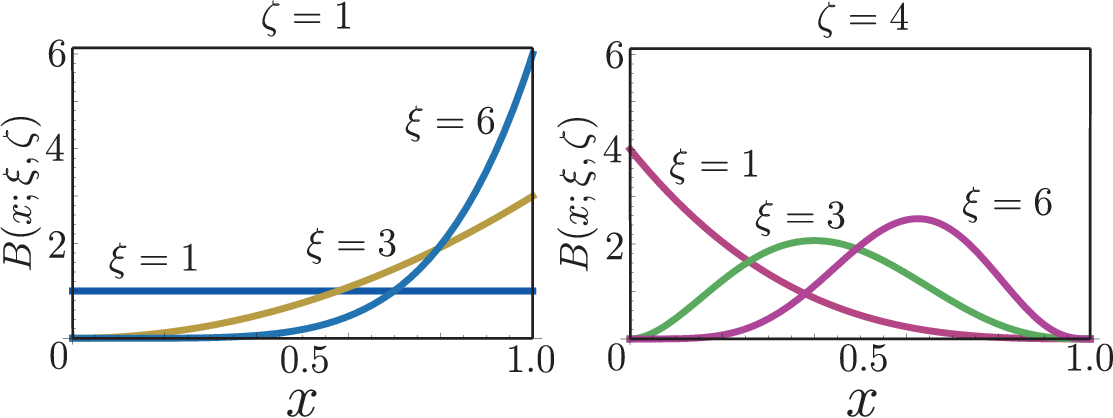
where ξ,ζ>0\xi,\zeta>0 are the shape parameters and Γ⁡(⋅)\Gamma(\cdot) denotes the Gamma function. Figure 4 plots B⁡(x,ξ,ζ)B(x;\xi,\zeta) for two values of ζ\zeta. The mean and variance of the Beta distribution (63) are given by

x¯=ξξ+ζ,σx2=ξ​ζ(ξ+ζ)2​(ξ+ζ+1)\bar{x}=\frac{\xi}{\xi+\zeta},\quad\sigma_{x}^{2}=\frac{\xi\zeta}{(\xi+\zeta)^{2}(\xi+\zeta+1)} (64)

For the asynchronous network model, we assume that the step-size 𝝁k​(i)\bm{\mu}_{k}(i) takes random values in the range [0,μk][0,\mu_{k}], where μk\mu_{k} denotes the largest possible value for the kk-th step-size. We further assume that the scaled parameter 𝝁k​(i)/μk\bm{\mu}_{k}(i)/\mu_{k} is governed by a Beta distribution:

𝒙k​(i)=𝝁k​(i)μk∼B⁡(xk,ξk,ζk)\bm{x}_{k}(i)=\frac{\bm{\mu}_{k}(i)}{\mu_{k}}\sim B(x_{k};\xi_{k},\zeta_{k}) (65)

where {ξk,ζk>0}\{\xi_{k},\zeta_{k}>0\} are the corresponding shape parameters. Likewise, we assume that the combination coefficient 𝒂ℓ​k​(i)\bm{a}_{\ell k}(i) for ℓ∈𝓝k,i\{k}\ell\in\bm{\mathcal{N}}_{k,i}\backslash\{k\} takes random values in the range [0,aℓ​k][0,a_{\ell k}] with 0<aℓ​k<10<a_{\ell k}<1. The scaled parameter 𝒂ℓ​k​(i)/aℓ​k\bm{a}_{\ell k}(i)/a_{\ell k} is assumed to be governed by a Beta distribution:

𝒚ℓ​k​(i)=𝒂ℓ​k​(i)aℓ​k∼B⁡(yℓ​k,ξℓ​k,ζℓ​k)\bm{y}_{\ell k}(i)=\frac{\bm{a}_{\ell k}(i)}{a_{\ell k}}\sim B(y_{\ell k};\xi_{\ell k},\zeta_{\ell k}) (66)

where {ξℓ​k,ζℓ​k>0}\{\xi_{\ell k},\zeta_{\ell k}>0\} are the shape parameters. We adopt the spatially uncorrelated model from Lemma 4. In order to guarantee that 𝒂k​k​(i)\bm{a}_{kk}(i) always assumes values within the range [0,1][0,1], we again require condition (57). Then, we can use (64) to calculate the relevant quantities introduced in the asynchronous network model:

μ¯k\displaystyle\bar{\mu}_{k} =ξkξk+ζk​μk\displaystyle=\frac{\xi_{k}}{\xi_{k}+\zeta_{k}}\mu_{k} (67)
cμ,k,k\displaystyle c_{\mu,k,k} =ξk​ζk(ξk+ζk)2​(ξk+ζk+1)​μk2\displaystyle=\frac{\xi_{k}\zeta_{k}}{(\xi_{k}+\zeta_{k})^{2}(\xi_{k}+\zeta_{k}+1)}\mu_{k}^{2} (68)
a¯ℓ​k\displaystyle\bar{a}_{\ell k} =ξℓ​kξℓ​k+ζℓ​k​aℓ​k\displaystyle=\frac{\xi_{\ell k}}{\xi_{\ell k}+\zeta_{\ell k}}a_{\ell k} (69)
a¯k​k\displaystyle\bar{a}_{kk} ≜1−∑ℓ∈𝒩\{k}ξℓ​kξℓ​k+ζℓ​k​aℓ​k\displaystyle\triangleq 1-\sum_{\ell\in\mathcal{N}\backslash\{k\}}\frac{\xi_{\ell k}}{\xi_{\ell k}+\zeta_{\ell k}}a_{\ell k} (70)
ca,ℓ​k,ℓ​k\displaystyle c_{a,\ell k,\ell k} =ξℓ​k​ζℓ​k(ξℓ​k+ζℓ​k)2​(ξℓ​k+ζℓ​k+1)​aℓ​k2,ℓ∈𝒩k\{k}\displaystyle=\frac{\xi_{\ell k}\zeta_{\ell k}}{(\xi_{\ell k}+\zeta_{\ell k})^{2}(\xi_{\ell k}+\zeta_{\ell k}+1)}a_{\ell k}^{2},\;\ell\in\mathcal{N}_{k}\backslash\{k\} (71)

IV Main Results

We presented a fairly general model for asynchronous events to cover many useful scenarios. Due to the random evolution of the step-sizes, topology, neighborhoods, and combination coefficients, the error dynamics of the network is influenced by more factors than traditional synchronous networks. Hence, before delving into the technical details, we summarize in this section some of the main conclusions that will follow from the analysis for the benefit of the reader.
Refer to caption
Fig. 4: The PDFs of the Beta distribution B⁡(x,ξ,ζ)B(x;\xi,\zeta) for different values of ξ\xi and ζ\zeta.

The first important result (in Part I) is Theorem 1, which presents in (93) a condition on the first and second-order moments of the random step-sizes to ensure the mean-square stability of the asynchronous network. It is noteworthy and also remarkable that the random distribution of the combination coefficients (and, hence, the randomness in the topology) does not affect the stability condition. This is another manifestation of the property stated earlier in the introduction, and which has been proven before only for synchronous networks in [15], that the mean-square stability of diffusion strategies is insensitive to the network topology even in the asynchronous case. Theorem 1 will show that studying the mean-square stability of the asynchronous network can be achieved by investigating the stability of the following recursive inequality:

maxk⁡𝔼​‖𝒘~k,i‖2≤β⋅maxk⁡𝔼​‖𝒘~k,i−1‖2+θ​σv2\max_{k}\mathbb{E}\|\widetilde{\bm{w}}_{k,i}\|^{2}\leq\beta\cdot\max_{k}\mathbb{E}\|\widetilde{\bm{w}}_{k,i-1}\|^{2}+\theta\sigma_{v}^{2} (72)

where 𝒘~k,i=wo−𝒘k,i\widetilde{\bm{w}}_{k,i}=w^{o}-\bm{w}_{k,i} denotes the error vector at agent kk at time ii, and {β,θ,σv2}\{\beta,\theta,\sigma_{v}^{2}\} are certain parameters defined by (90), (91), and (25), respectively. The recursive inequality (72) provides an upper bound for the worst individual MSD in the network at every time ii. Thus, as long as the factor β\beta is inside the unit circle, i.e., |β|<1|\beta|<1, then the sequences {𝔼​‖𝒘~k,i‖2;i≥0}\{\mathbb{E}\|\widetilde{\bm{w}}_{k,i}\|^{2};i\geq 0\} for all kk will remain bounded and the network will be mean-square stable. Theorem 1 provides a sufficient condition to guarantee |β|<1|\beta|<1. The condition involves the first and second-order moments of the step-size distribution as follows:

μ¯k2+cμ,k,kμ¯k<λk,minα+λk,max2\frac{\bar{\mu}_{k}^{2}+c_{\mu,k,k}}{\bar{\mu}_{k}}<\frac{\lambda_{k,\min}}{\alpha+\lambda_{k,\max}^{2}} (73)

for all kk, where {λk,min,λk,max}\{\lambda_{k,\min},\lambda_{k,\max}\} and α\alpha are from Assumptions 2 and 3, respectively. As long as condition (73) holds, the random step-sizes will lead to stable networks regardless of their PDFs. Furthermore, when condition (73) holds, the same theorem establishes that the MSD of the individual agents will eventually be bounded by

lim supi→∞𝔼​‖𝒘~k,i‖2≤b⋅νo\limsup_{i\rightarrow\infty}\mathbb{E}\|\widetilde{\bm{w}}_{k,i}\|^{2}\leq b\cdot\nu_{o} (74)

where bb and νo\nu_{o} are given by (95) and νo\nu_{o} is reproduced here:

νo=maxk⁡μ¯k2+cμ,k,kμ¯k=μ¯k(2)μ¯k(1)\nu_{o}=\max_{k}\frac{\bar{\mu}_{k}^{2}+c_{\mu,k,k}}{\bar{\mu}_{k}}=\frac{\bar{\mu}_{k}^{(2)}}{\bar{\mu}_{k}^{(1)}} (75)

where μ¯k(m)≜𝔼​[𝝁k​(i)]m\bar{\mu}_{k}^{(m)}\triangleq\mathbb{E}[\bm{\mu}_{k}(i)]^{m} denotes the mm-th moment of 𝝁k​(i)\bm{\mu}_{k}(i) and μ¯k≡μ¯k(1)\bar{\mu}_{k}\equiv\bar{\mu}_{k}^{(1)}. Thus, the individual MSD values will decrease with νo\nu_{o} and can become arbitrarily small in steady-state.

With some strengthened assumptions on the gradient noise and random step-sizes, and using Theorem 1, we then establish in Part II [2] two important conclusions:

limi→∞𝔼​‖wo−𝒘k,i‖2\displaystyle\lim_{i\rightarrow\infty}\mathbb{E}\,\|w^{o}-\bm{w}_{k,i}\|^{2} =O⁡(ν)\displaystyle=O(\nu) (76)
limi→∞𝔼​‖𝒘k,i−𝒘ℓ,i‖2\displaystyle\lim_{i\rightarrow\infty}\mathbb{E}\,\|\bm{w}_{k,i}-\bm{w}_{\ell,i}\|^{2} =O⁡(ν1+γo′)\displaystyle=O(\nu^{1+\gamma_{o}^{\prime}}) (77)

for some γo′>0\gamma_{o}^{\prime}>0 and sufficiently small ν\nu. The parameter ν\nu is defined by

ν≜maxk⁡μ¯k(4)μ¯k(1)\nu\triangleq\max_{k}\frac{\sqrt{\bar{\mu}_{k}^{(4)}}}{\bar{\mu}_{k}^{(1)}} (78)

These results imply that all agents reach a level of O⁡(ν1+γo′)O(\nu^{1+\gamma_{o}^{\prime}}) agreement with each other and get O⁡(ν)O(\nu) close to the desired solution wow^{o} in steady-state. This interesting behavior is illustrated in Fig. 5, where it is shown that, despite being subjected to different sources of randomness and failures, the agents in an asynchronous network are still able to approach the desired solution and they are also able to coalesce close to each other while seeking the desired solution. Actually, in Part II [2], we shall derive explicit closed-form expressions for the size of the error variances in (76) and (77).

V Mean-Square Stability

For each agent kk, we introduce the error vectors:

𝝍~k,i≜wo−𝝍k,i,𝒘~k,i≜wo−𝒘k,i\widetilde{\bm{\psi}}_{k,i}\triangleq w^{o}-\bm{\psi}_{k,i},\qquad\widetilde{\bm{w}}_{k,i}\triangleq w^{o}-\bm{w}_{k,i} (79)

where wow^{o} is the desired optimal solution. Subtracting wow^{o} from both sides of (16a)–(16b) and using (18) gives

𝝍~k,i\displaystyle\widetilde{\bm{\psi}}_{k,i} =𝒘~k,i−1+𝝁k​(i)​[∇w∗Jk​(𝒘k,i−1)+𝒗k,i​(𝒘k,i−1)]\displaystyle=\widetilde{\bm{w}}_{k,i-1}+\bm{\mu}_{k}(i)[\nabla_{w^{*}}J_{k}(\bm{w}_{k,i-1})+\bm{v}_{k,i}(\bm{w}_{k,i-1})] (80a)
𝒘~k,i\displaystyle\widetilde{\bm{w}}_{k,i} =∑ℓ∈𝓝k,i𝒂ℓ​k​(i)​𝝍~ℓ,i\displaystyle=\sum_{\ell\in\bm{\mathcal{N}}_{k,i}}\bm{a}_{\ell k}(i)\,\widetilde{\bm{\psi}}_{\ell,i} (80b)

Applying the transformation 𝕋¯​(⋅)\underaccent{\bar}{\mbbT}(\cdot) from (4) to both sides of these equations, we show in Appendix C that the error recursion (80a)–(80b) becomes

𝝍¯~k,i\displaystyle\underaccent{\bar}{\wt{\bm{\psi}}}_{k,i} =[I2​M−𝝁k​(i)​𝑯k,i−1]​𝒘¯~k,i−1+𝝁k​(i)​𝒗¯k,i​(𝒘k,i−1)\displaystyle=[I_{2M}-\bm{\mu}_{k}(i)\bm{H}_{k,i-1}]\underaccent{\bar}{\wt{\bm{w}}}_{k,i-1}+\bm{\mu}_{k}(i)\underaccent{\bar}{\bm{v}}_{k,i}(\bm{w}_{k,i-1}) (81a)
𝒘¯~k,i\displaystyle\underaccent{\bar}{\wt{\bm{w}}}_{k,i} =∑ℓ∈𝓝k,i𝒂ℓ​k​(i)​𝝍¯~ℓ,i\displaystyle=\sum_{\ell\in\bm{\mathcal{N}}_{k,i}}\bm{a}_{\ell k}(i)\,\underaccent{\bar}{\wt{\bm{\psi}}}_{\ell,i} (81b)

where we introduced the 2​M×2​M2M\times 2M matrix:

𝑯k,i−1≜∫01∇w¯​w¯∗2​Jk​(w¯o−t​𝒘¯~k,i−1)​𝑑t\bm{H}_{k,i-1}\triangleq\int_{0}^{1}\nabla_{\underaccent{\bar}{w}\underaccent{\bar}{w}^{*}}^{2}J_{k}(\underaccent{\bar}{w}^{o}-t\underaccent{\bar}{\wt{\bm{w}}}_{k,i-1})\,dt (82)

To proceed, we introduce the following network variables:

𝒘¯~i\displaystyle\underaccent{\bar}{\wt{\bm{w}}}_{i} ≜col⁡{𝒘¯~1,i,𝒘¯~2,i,…,𝒘¯~N,i}\displaystyle\triangleq{\mathrm{col}}\{\underaccent{\bar}{\wt{\bm{w}}}_{1,i},\underaccent{\bar}{\wt{\bm{w}}}_{2,i},\dots,\underaccent{\bar}{\wt{\bm{w}}}_{N,i}\} (83)
𝓜i\displaystyle\bm{\mathcal{M}}_{i} ≜𝑴i⊗I2​M\displaystyle\triangleq\bm{M}_{i}\otimes I_{2M} (84)
𝓐i\displaystyle\bm{\mathcal{A}}_{i} ≜𝑨i⊗I2​M\displaystyle\triangleq\bm{A}_{i}\otimes I_{2M} (85)
𝓗i\displaystyle\bm{\mathcal{H}}_{i} ≜diag⁡{𝑯1,i,𝑯2,i,…,𝑯N,i}\displaystyle\triangleq{\mathrm{diag}}\{\bm{H}_{1,i},\bm{H}_{2,i},\dots,\bm{H}_{N,i}\} (86)

Using (81a)–(81b) we conclude that the network error vector (83) evolves according to the following dynamics:

𝒘¯~i=𝓐i𝖳​(I2​M​N−𝓜i​𝓗i−1)​𝒘¯~i−1+𝓐i𝖳​𝓜i​𝒗¯i​(𝒘i−1)\boxed{\underaccent{\bar}{\wt{\bm{w}}}_{i}=\bm{\mathcal{A}}_{i}^{\mathsf{T}}(I_{2MN}-\bm{\mathcal{M}}_{i}\bm{\mathcal{H}}_{i-1})\underaccent{\bar}{\wt{\bm{w}}}_{i-1}+\bm{\mathcal{A}}_{i}^{\mathsf{T}}\bm{\mathcal{M}}_{i}\underaccent{\bar}{\bm{v}}_{i}(\bm{w}_{i-1})} (87)
Refer to caption
Fig. 5: Illustration for results (76) and (77): the solutions by the agents do not only get O⁡(ν)O(\nu) close to the target wow^{o} but they also cluster next to each other within O⁡(ν1+γo′)O(\nu^{1+\gamma_{o}^{\prime}}) for some γo′>0\gamma_{o}^{\prime}>0.

V-A Condition for Mean-Square Stability

The main result in this Part I is to establish the mean-square stability of this recursion in Theorem 1 below. The difficulty lies in the fact that the error dynamics (87) is a time-variant stochastic recursion that also depends nonlinearly on the data. The parameters {𝓐i,𝓜i,𝓗i−1}\{\bm{\mathcal{A}}_{i},\bm{\mathcal{M}}_{i},\bm{\mathcal{H}}_{i-1}\} are random, time-varying, and multiplied together and by the error vector and noise variables. The statement and proof of Theorem 1 rely on the following quantities:

ϵ2​(i)\displaystyle\epsilon^{2}(i) ≜maxk⁡𝔼​‖𝒘~k,i‖2=12⋅maxk⁡𝔼​‖𝒘¯~k,i‖2\displaystyle\triangleq\max_{k}\mathbb{E}\|\widetilde{\bm{w}}_{k,i}\|^{2}=\frac{1}{2}\cdot\max_{k}\mathbb{E}\|\underaccent{\bar}{\wt{\bm{w}}}_{k,i}\|^{2} (88)
γk2\displaystyle\gamma_{k}^{2} ≜1−2​μ¯k​λk,min+(μ¯k2+cμ,k,k)​λk,max2\displaystyle\triangleq 1-2\bar{\mu}_{k}\lambda_{k,\min}+(\bar{\mu}_{k}^{2}+c_{\mu,k,k})\lambda_{k,\max}^{2} (89)
β\displaystyle\beta ≜maxk⁡{γk2+α⁡(μ¯k2+cμ,k,k)}\displaystyle\triangleq\max_{k}\{\gamma_{k}^{2}+\alpha(\bar{\mu}_{k}^{2}+c_{\mu,k,k})\} (90)
θ\displaystyle\theta ≜maxk⁡{μ¯k2+cμ,k,k}\displaystyle\triangleq\max_{k}\{\bar{\mu}_{k}^{2}+c_{\mu,k,k}\} (91)

where the {λk,min,λk,max}\{\lambda_{k,\min},\lambda_{k,\max}\} correspond to the lower and upper bounds on the Hessian matrices from (8).

Theorem 1 (Mean-square stability)

The mean-square stability of the asynchronous diffusion strategy (28a)–(28b) reduces to studying the convergence of the recursive inequality:

ϵ2​(i)≤β⋅ϵ2​(i−1)+θ​σv2\epsilon^{2}(i)\leq\beta\cdot\epsilon^{2}(i-1)+\theta\sigma_{v}^{2} (92)

where σv2\sigma_{v}^{2} is from (25). The model (92) is stable if the mean {μ¯k}\{\bar{\mu}_{k}\} and the ratio {(μ¯k2+cμ,k,k)/μ¯k}\{(\bar{\mu}_{k}^{2}+c_{\mu,k,k})/\bar{\mu}_{k}\} satisfy the following relation:

μ¯k2+cμ,k,kμ¯k<λk,minα+λk,max2\boxed{\frac{\bar{\mu}_{k}^{2}+c_{\mu,k,k}}{\bar{\mu}_{k}}<\frac{\lambda_{k,\min}}{\alpha+\lambda_{k,\max}^{2}}} (93)

for k=1,2,…,Nk=1,2,\dots,N, where the parameter α\alpha is from (27). When condition (93) holds, an upper bound on the individual steady-state mean-square-deviation (MSD) for each agent kk in the network is given by

lim supi→∞𝔼​‖𝒘~k,i‖2≤b⋅νo\boxed{\limsup_{i\rightarrow\infty}\mathbb{E}\|\widetilde{\bm{w}}_{k,i}\|^{2}\leq b\cdot\nu_{o}} (94)

where

νo≜maxk⁡μ¯k2+cμ,k,kμ¯k,b≜κ​σv2mink⁡{λk,min}\nu_{o}\triangleq\max_{k}\frac{\bar{\mu}_{k}^{2}+c_{\mu,k,k}}{\bar{\mu}_{k}},\quad b\triangleq\frac{\kappa\sigma_{v}^{2}}{\min_{k}\{\lambda_{k,\min}\}} (95)

and the parameter κ\kappa is from (38).

Proof:

See Appendix D. ∎

From the asynchronous network model, we know that 𝝁k​(i)∈[0,μk]\bm{\mu}_{k}(i)\in[0,\mu_{k}]. It follows that

μ¯k2+cμ,k,kμ¯k=μ¯k(2)μ¯k(1)≤𝔼⁡[𝝁k​(i)​μk]μ¯k=μk\frac{\bar{\mu}_{k}^{2}+c_{\mu,k,k}}{\bar{\mu}_{k}}=\frac{\bar{\mu}_{k}^{(2)}}{\bar{\mu}_{k}^{(1)}}\leq\frac{\mathbb{E}\,[\bm{\mu}_{k}(i)\mu_{k}]}{\bar{\mu}_{k}}=\mu_{k} (96)

From (96), a sufficient condition for (93) to hold is given by

μk<λk,minα+λk,max2\mu_{k}<\frac{\lambda_{k,\min}}{\alpha+\lambda_{k,\max}^{2}} (97)

Condition (93) allows us to provide some insights about how the dispersion of 𝝁k​(i)\bm{\mu}_{k}(i) affects mean-square stability. Note that condition (93) even allows the random step-sizes to assume some abnormally large values at a relatively low probability. This “hopping” behavior (resulting from infrequent large step-sizes) would not destroy the mean-square stability of the network; this fact reveals another useful form of robustness.

Since the constant coefficient bb defined in (95) is a fixed bound, Theorem 1 implies that for sufficiently large ii, the MSD of each individual agent’s solution has a bounded value. The upper bound in (94) is proportional to the parameter νo\nu_{o} across the network. Using the useful conclusion of (94), we will be able to derive in the sequel a condition for fourth-order stability of the error recursion (87).

V-B Stability Conditions for Bernoulli and Beta Models

We specialize condition (94) for the asynchronous models described in Section III-D.

V-B1 The Bernoulli Model

Substituting (58) and (59) into (93) yields the condition

μk<λk,minα+λk,max2\mu_{k}<\frac{\lambda_{k,\min}}{\alpha+\lambda_{k,\max}^{2}} (98)

which is identical to condition (97) on the upper limit of the range of random step-sizes.

V-B2 The Beta Model

Without loss of generality, let ζk=ϕk⋅ξk\zeta_{k}=\phi_{k}\cdot\xi_{k} with a constant factor ϕk>0\phi_{k}>0. It follows from (67) that the mean value μ¯k\bar{\mu}_{k} can be expressed in terms of the factor ϕk\phi_{k} and the upper limit μk\mu_{k}:

μ¯k=μk1+ϕk\bar{\mu}_{k}=\frac{\mu_{k}}{1+\phi_{k}} (99)

Likewise, from (68), we have

cμ,k,k=ϕk​μk2(1+ϕk)2​(ξk+ξk​ϕk+1)c_{\mu,k,k}=\frac{\phi_{k}\mu_{k}^{2}}{(1+\phi_{k})^{2}(\xi_{k}+\xi_{k}\phi_{k}+1)} (100)

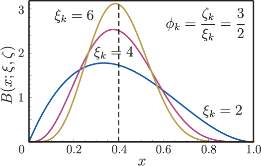
which is a monotonically decreasing function of the shape parameter ξk≥1\xi_{k}\geq 1. As the value of ξk\xi_{k} becomes larger, the probability mass of 𝝁k​(i)\bm{\mu}_{k}(i) will gradually concentrate around its mean (99), as shown in Fig. 6. Substituting (99) and (100) into (93) yields

μk<(1+ϕk​ξk1+ξk)​λk,minα+λk,max2\mu_{k}<\left(1+\frac{\phi_{k}\xi_{k}}{1+\xi_{k}}\right)\frac{\lambda_{k,\min}}{\alpha+\lambda_{k,\max}^{2}} (101)

where μk\mu_{k} is the largest possible value for 𝝁k​(i)\bm{\mu}_{k}(i) defined by (65). In (101), the bound on μk\mu_{k} is a monotonically increasing function of the shape parameter ξk≥1\xi_{k}\geq 1. As ξk\xi_{k} becomes larger, the bound in (101) becomes larger. The net effect allows for a wider range for the realizations of the random step-sizes. Moreover, it is easy to verify that the upper bound in (101) is larger than that in (98).

V-C Condition for Fourth-Order Stability

Result (94) establishes that the network is mean-square stable under the assumption of bounded second-order moments for the gradient noise process as in (27). If desired, under a similar condition on bounded fourth-order moments for the gradient noise, we can also establish by extending the arguments of Appendix D and [57] that the error recursion (87) is stable in the fourth-order sense.

Theorem 2 (Stability of fourth-order error moments)

Assume the fourth-order moments of the gradient noise components are bounded by

𝔼⁡[‖𝒗k,i​(𝒘k,i−1)‖4|𝔽i−1]≤α2​‖wo−𝒘k,i−1‖4+σv4\mathbb{E}[\|\bm{v}_{k,i}(\bm{w}_{k,i-1})\|^{4}|\mathbb{F}_{i-1}]\leq\alpha^{2}\|w^{o}-\bm{w}_{k,i-1}\|^{4}+\sigma_{v}^{4} (102)

for some constants α≥0\alpha\geq 0 and σv≥0\sigma_{v}\geq 0. If

μ¯k(4)μ¯k<λk,min3​λk,max2+4​α\frac{\sqrt{\bar{\mu}_{k}^{(4)}}}{\bar{\mu}_{k}}<\frac{\lambda_{k,\min}}{3\lambda_{k,\max}^{2}+4\alpha} (103)

holds for all kk, then the fourth-order moments of the individual errors are asymptotically bounded by

lim supi→∞𝔼​‖𝒘~k,i‖4≤b42⋅ν2\boxed{\limsup_{i\rightarrow\infty}\mathbb{E}\|\widetilde{\bm{w}}_{k,i}\|^{4}\leq b_{4}^{2}\cdot\nu^{2}} (104)

where the parameter ν\nu is defined by

ν≜maxk⁡μ¯k(4)μ¯k,b4≜3​σv2​(κ+1)mink⁡λk,min\nu\triangleq\max_{k}\frac{\sqrt{\bar{\mu}_{k}^{(4)}}}{\bar{\mu}_{k}},\quad b_{4}\triangleq\frac{3\sigma_{v}^{2}(\kappa+1)}{\min_{k}\lambda_{k,\min}} (105)
Proof:

See Appendix E. ∎

Refer to caption
Fig. 6: The PDFs of the Beta distribution B⁡(x,ξk,ζk)B(x;\xi_{k},\zeta_{k}) for ζk=1.5​ξk\zeta_{k}=1.5\xi_{k} and ξk=2,4,6\xi_{k}=2,4,6.

It is easy to verify that condition (102) implies a bound on the second-order moment of the gradient noise:

𝔼⁡[‖𝒗k,i​(𝒘k,i−1)‖2|𝔽i−1]≤α​‖wo−𝒘k,i−1‖2+σv2\mathbb{E}[\|\bm{v}_{k,i}(\bm{w}_{k,i-1})\|^{2}|\mathbb{F}_{i-1}]\leq\alpha\|w^{o}-\bm{w}_{k,i-1}\|^{2}+\sigma_{v}^{2} (106)

although the converse is generally not true. In other words, it is redundant to assume both conditions (27) and (102). It can be verified that condition (103) implies (93) (see (200) and (201) in Appendix E). Therefore, conditions (102) and (103) are sufficient to ensure both mean-square and fourth-order stability of error moments. Moreover, it is straightforward to verify that

νo=maxk⁡μ¯k(2)μ¯k≤maxk⁡μ¯k(4)μ¯k=ν\nu_{o}=\max_{k}\frac{\bar{\mu}_{k}^{(2)}}{\bar{\mu}_{k}}\leq\max_{k}\frac{\sqrt{\bar{\mu}_{k}^{(4)}}}{\bar{\mu}_{k}}=\nu (107)

Therefore, we can use ν\nu to upper bound νo\nu_{o}.

VI Conclusion

We introduced a fairly general model for asynchronous behavior over networks with random step-sizes, links, topologies, and combination coefficients. We then carried out a mean-square analysis and showed that, even under non-vanishing step-sizes, the asynchronous network remains mean-square stable for sufficiently small step-sizes. We derived a condition on the first and second-order moments of the random step-sizes to ensure stable behavior. We specialized the results to two models: a Bernoulli network and a Beta network. It was observed that the Beta network admits a wider range of step-sizes for stability. The results suggest that networks where step-sizes assume values randomly within a certain interval are robustly more stable than networks that have their step-sizes be turned on or off. In Part II [2] of this work, we derive explicit closed-form expressions for the MSD performance and use these expressions to clarify how the parameters of the asynchronous behavior influence both the convergence rate and the MSE performance. We will also be able to establish the useful clustering property illustrated by Fig. 5, namely, that the iterates at the various agents approach the optimal solution within accuracy O⁡(ν)O(\nu) while clustering close to each other within O⁡(ν1+γo′)O(\nu^{1+\gamma_{o}^{\prime}}) for some γo′>0\gamma_{o}^{\prime}>0.

Appendix A Equivalent Complex-Domain Representations

First, we recall the definition of the real Jacobian of a real-valued function J⁡(w)J(w) with respect to a real column vector w∈ℝMw\in\mathbb{R}^{M} as

∂J⁡(w)∂w≜row⁡{∂J⁡(w)∂w1,∂J⁡(w)∂w2,…,∂J⁡(w)∂wM}\frac{\partial J(w)}{\partial w}\triangleq{\mathrm{row}}\left\{\frac{\partial J(w)}{\partial w_{1}},\frac{\partial J(w)}{\partial w_{2}},\dots,\frac{\partial J(w)}{\partial w_{M}}\right\} (108)

where wm∈ℝw_{m}\in\mathbb{R} denotes the mm-th element of ww. Using (2), the real gradient of the function Jk​(w¯)J_{k}(\bar{w}) with respect to w¯\bar{w} is defined as

∇w¯Jk​(w¯)≜∂Jk​(w¯)∂w¯=[∂Jk​(w)∂ℜ​𝔢​(w)∂Jk​(w)∂ℑ​𝔪​(w)]\nabla_{\bar{w}}J_{k}(\bar{w})\triangleq\frac{\partial J_{k}(\bar{w})}{\partial\bar{w}}=\begin{bmatrix}\frac{\partial J_{k}(w)}{\partial\mathfrak{Re}(w)}&\frac{\partial J_{k}(w)}{\partial\mathfrak{Im}(w)}\end{bmatrix} (109)

and the real Hessian matrix of the same function Jk​(w¯)J_{k}(\bar{w}) with respect to w¯\bar{w} is defined by

∇w¯​w¯𝖳2​Jk​(w¯)≜∂∂w¯​[∂Jk​(w¯)∂w¯]𝖳=[∂∂ℜ​𝔢​(w)​[∂Jk​(w)∂ℜ​𝔢​(w)]𝖳∂∂ℑ​𝔪​(w)​[∂Jk​(w)∂ℜ​𝔢​(w)]𝖳∂∂ℜ​𝔢​(w)​[∂Jk​(w)∂ℑ​𝔪​(w)]𝖳∂∂ℑ​𝔪​(w)​[∂Jk​(w)∂ℑ​𝔪​(w)]𝖳]\displaystyle\nabla_{\bar{w}\bar{w}^{\mathsf{T}}}^{2}J_{k}(\bar{w})\triangleq\frac{\partial}{\partial\bar{w}}\left[\frac{\partial J_{k}(\bar{w})}{\partial\bar{w}}\right]^{\mathsf{T}}=\begin{bmatrix}\frac{\partial}{\partial\mathfrak{Re}(w)}\left[\frac{\partial J_{k}(w)}{\partial\mathfrak{Re}(w)}\right]^{\mathsf{T}}&\frac{\partial}{\partial\mathfrak{Im}(w)}\left[\frac{\partial J_{k}(w)}{\partial\mathfrak{Re}(w)}\right]^{\mathsf{T}}\\ \frac{\partial}{\partial\mathfrak{Re}(w)}\left[\frac{\partial J_{k}(w)}{\partial\mathfrak{Im}(w)}\right]^{\mathsf{T}}&\frac{\partial}{\partial\mathfrak{Im}(w)}\left[\frac{\partial J_{k}(w)}{\partial\mathfrak{Im}(w)}\right]^{\mathsf{T}}\\ \end{bmatrix} (110)

It is easy to verify that ∇w¯​w¯𝖳2​Jk​(w¯)\nabla_{\bar{w}\bar{w}^{\mathsf{T}}}^{2}J_{k}(\bar{w}) is a symmetric matrix.

Then, we define the derivative of a real-valued function J⁡(z)J(z) with respect to the complex argument z∈ℂz\in\mathbb{C} as [58, 59]:

∂J⁡(z)∂z≜12​(∂J⁡(z)∂ℜ​𝔢​(z)−j​∂J⁡(z)∂ℑ​𝔪​(z))\frac{\partial J(z)}{\partial z}\triangleq\frac{1}{2}\left(\frac{\partial J(z)}{\partial\mathfrak{Re}(z)}-j\frac{\partial J(z)}{\partial\mathfrak{Im}(z)}\right) (111)

and the complex Jacobian of a real-valued function J⁡(w)J(w) with respect to the complex column vector w∈ℂMw\in\mathbb{C}^{M} is given by

∂J⁡(w)∂w≜row⁡{∂J⁡(w)∂w1,∂J⁡(w)∂w2,…,∂J⁡(w)∂wM}\frac{\partial J(w)}{\partial w}\triangleq{\mathrm{row}}\left\{\frac{\partial J(w)}{\partial w_{1}},\frac{\partial J(w)}{\partial w_{2}},\dots,\frac{\partial J(w)}{\partial w_{M}}\right\} (112)

where wm∈ℂw_{m}\in\mathbb{C} denotes the mm-th element of ww. The complex gradient of the real-valued function Jk​(w)J_{k}(w) with respect to the complex vector argument w∈ℂMw\in\mathbb{C}^{M} is defined as [59, eq. (20)] (compare with (109)):

∇wJk​(w)≜∂J⁡(w)∂w=12​(∂J⁡(w)∂ℜ​𝔢​(w)−j​∂J⁡(w)∂ℑ​𝔪​(w))\nabla_{w}J_{k}(w)\triangleq\frac{\partial J(w)}{\partial w}=\frac{1}{2}\left(\frac{\partial J(w)}{\partial\mathfrak{Re}(w)}-j\frac{\partial J(w)}{\partial\mathfrak{Im}(w)}\right) (113)

and the complex conjugate gradient of Jk​(w)J_{k}(w) with respect to w∗∈ℂMw^{*}\in\mathbb{C}^{M} is defined by [59, eqs. (21, 22)]:

∇w∗Jk​(w)≜∂J⁡(w)∂w∗=[∇wJk​(w)]∗\nabla_{w^{*}}J_{k}(w)\triangleq\frac{\partial J(w)}{\partial w^{*}}=\left[\nabla_{w}J_{k}(w)\right]^{*} (114)

Using (4), the complex gradient of Jk​(w¯)J_{k}(\underaccent{\bar}{w}) with respect to the column vector w¯∈ℂM2​M\underaccent{\bar}{w}\in\mathbb{C}_{M}^{2M} is then given by [59, eq. (18)]:

∇w¯Jk​(w¯)=∂Jk​(w¯)∂w¯=[∇wJk​(w)(∇w∗Jk​(w))𝖳]\nabla_{\underaccent{\bar}{w}}J_{k}(\underaccent{\bar}{w})=\frac{\partial J_{k}(\underaccent{\bar}{w})}{\partial\underaccent{\bar}{w}}=\begin{bmatrix}\nabla_{w}J_{k}(w)&(\nabla_{w^{*}}J_{k}(w))^{\mathsf{T}}\\ \end{bmatrix} (115)

and the corresponding complex conjugate gradient is given by

∇w¯∗Jk​(w¯)=[∂Jk​(w¯)∂w¯]∗=[∇w¯Jk​(w¯)]∗\nabla_{\underaccent{\bar}{w}^{*}}J_{k}(\underaccent{\bar}{w})=\left[\frac{\partial J_{k}(\underaccent{\bar}{w})}{\partial\underaccent{\bar}{w}}\right]^{*}=[\nabla_{\underaccent{\bar}{w}}J_{k}(\underaccent{\bar}{w})]^{*} (116)

The complex Hessian of Jk​(w¯)J_{k}(\underaccent{\bar}{w}) with respect to w¯∈ℂM2​M\underaccent{\bar}{w}\in\mathbb{C}_{M}^{2M} is defined by [59, eq. (32)]:

∇w¯​w¯∗2​Jk​(w¯)\displaystyle\nabla_{\underaccent{\bar}{w}\underaccent{\bar}{w}^{*}}^{2}J_{k}(\underaccent{\bar}{w}) ≜∂∂w¯​[∂Jk​(w¯)∂w¯]∗\displaystyle\triangleq\frac{\partial}{\partial\underaccent{\bar}{w}}\left[\frac{\partial J_{k}(\underaccent{\bar}{w})}{\partial\underaccent{\bar}{w}}\right]^{*}{}
=[∇w​w∗2​Jk​(w)(∇w​w𝖳2​Jk​(w))∗∇w​w𝖳2​Jk​(w)(∇w​w∗2​Jk​(w))𝖳]\displaystyle=\begin{bmatrix}\nabla_{ww^{*}}^{2}J_{k}(w)&(\nabla_{ww^{\mathsf{T}}}^{2}J_{k}(w))^{*}\\ \nabla_{ww^{\mathsf{T}}}^{2}J_{k}(w)&(\nabla_{ww^{*}}^{2}J_{k}(w))^{\mathsf{T}}\\ \end{bmatrix} (117)

where

∇w​w∗2​Jk​(w)\displaystyle\nabla_{ww^{*}}^{2}J_{k}(w) ≜∂∂w​[∂Jk​(w)∂w]∗=[∂2Jk​(w)∂w1∗​∂w1∂2Jk​(w)∂w1∗​∂w2…∂2Jk​(w)∂w1∗​∂wM∂2Jk​(w)∂w2∗​∂w1∂2Jk​(w)∂w2∗​∂w2…∂2Jk​(w)∂w2∗​∂wM⋱∂2Jk​(w)∂wM∗​∂w1∂2Jk​(w)∂wM∗​∂w2…∂2Jk​(w)∂wM∗​∂wM]\displaystyle\triangleq\frac{\partial}{\partial w}\left[\frac{\partial J_{k}(w)}{\partial w}\right]^{*}=\begin{bmatrix}\frac{\partial^{2}J_{k}(w)}{\partial w_{1}^{*}\partial w_{1}}&\frac{\partial^{2}J_{k}(w)}{\partial w_{1}^{*}\partial w_{2}}&\dots&\frac{\partial^{2}J_{k}(w)}{\partial w_{1}^{*}\partial w_{M}}\\ \frac{\partial^{2}J_{k}(w)}{\partial w_{2}^{*}\partial w_{1}}&\frac{\partial^{2}J_{k}(w)}{\partial w_{2}^{*}\partial w_{2}}&\dots&\frac{\partial^{2}J_{k}(w)}{\partial w_{2}^{*}\partial w_{M}}\\ \vdots&\vdots&\ddots&\vdots\\ \frac{\partial^{2}J_{k}(w)}{\partial w_{M}^{*}\partial w_{1}}&\frac{\partial^{2}J_{k}(w)}{\partial w_{M}^{*}\partial w_{2}}&\dots&\frac{\partial^{2}J_{k}(w)}{\partial w_{M}^{*}\partial w_{M}}\\ \end{bmatrix} (118)
∇w​w𝖳2​Jk​(w)\displaystyle\nabla_{ww^{\mathsf{T}}}^{2}J_{k}(w) ≜∂∂w​[∂Jk​(w)∂w]𝖳=[∂2Jk​(w)∂w1​∂w1∂2Jk​(w)∂w1​∂w2…∂2Jk​(w)∂w1​∂wM∂2Jk​(w)∂w2​∂w1∂2Jk​(w)∂w2​∂w2…∂2Jk​(w)∂w2​∂wM⋱∂2Jk​(w)∂wM​∂w1∂2Jk​(w)∂wM​∂w2…∂2Jk​(w)∂wM​∂wM]\displaystyle\triangleq\frac{\partial}{\partial w}\left[\frac{\partial J_{k}(w)}{\partial w}\right]^{\mathsf{T}}=\begin{bmatrix}\frac{\partial^{2}J_{k}(w)}{\partial w_{1}\partial w_{1}}&\frac{\partial^{2}J_{k}(w)}{\partial w_{1}\partial w_{2}}&\dots&\frac{\partial^{2}J_{k}(w)}{\partial w_{1}\partial w_{M}}\\ \frac{\partial^{2}J_{k}(w)}{\partial w_{2}\partial w_{1}}&\frac{\partial^{2}J_{k}(w)}{\partial w_{2}\partial w_{2}}&\dots&\frac{\partial^{2}J_{k}(w)}{\partial w_{2}\partial w_{M}}\\ \vdots&\vdots&\ddots&\vdots\\ \frac{\partial^{2}J_{k}(w)}{\partial w_{M}\partial w_{1}}&\frac{\partial^{2}J_{k}(w)}{\partial w_{M}\partial w_{2}}&\dots&\frac{\partial^{2}J_{k}(w)}{\partial w_{M}\partial w_{M}}\\ \end{bmatrix} (119)

It is easy to verify that ∇w¯​w¯∗2​Jk​(w¯)\nabla_{\underaccent{\bar}{w}\underaccent{\bar}{w}^{*}}^{2}J_{k}(\underaccent{\bar}{w}) is a Hermitian matrix.

From (109) and (115), we have [59, eqs. (18, 19)]:

∇w¯Jk​(w¯)\displaystyle\nabla_{\bar{w}}J_{k}(\bar{w}) =∇w¯Jk​(w¯)⋅D\displaystyle=\nabla_{\underaccent{\bar}{w}}J_{k}(\underaccent{\bar}{w})\cdot D (120)
∇w¯Jk​(w¯)⋅12​D∗\displaystyle\nabla_{\bar{w}}J_{k}(\bar{w})\cdot\frac{1}{2}D^{*} =∇w¯Jk​(w¯)\displaystyle=\nabla_{\underaccent{\bar}{w}}J_{k}(\underaccent{\bar}{w}) (121)

Similarly, from (110) and (117), we have [59, eqs. (32, 33)]:

∇w¯​w¯𝖳2​Jk​(w¯)\displaystyle\nabla_{\bar{w}\bar{w}^{\mathsf{T}}}^{2}J_{k}(\bar{w}) =D∗⋅[∇w¯​w¯∗2​Jk​(w¯)]⋅D\displaystyle=D^{*}\cdot[\nabla_{\underaccent{\bar}{w}\underaccent{\bar}{w}^{*}}^{2}J_{k}(\underaccent{\bar}{w})]\cdot D (122)
14​D⋅[∇w¯​w¯𝖳2​Jk​(w¯)]⋅D∗\displaystyle\frac{1}{4}D\cdot[\nabla_{\bar{w}\bar{w}^{\mathsf{T}}}^{2}J_{k}(\bar{w})]\cdot D^{*} =∇w¯​w¯∗2​Jk​(w¯)\displaystyle=\nabla_{\underaccent{\bar}{w}\underaccent{\bar}{w}^{*}}^{2}J_{k}(\underaccent{\bar}{w}) (123)

Identities (120)–(123) play an important role in our analysis.

Appendix B Proof of Lemma 4

Expression (50) is because 𝝁k​(i)\bm{\mu}_{k}(i) and 𝝁ℓ​(i)\bm{\mu}_{\ell}(i) are uncorrelated when k≠ℓk\neq\ell. Expression (52) is obtained by using (50) and (36). Using (29) and Lemma 2, we have

𝒂k​k​(i)=1−∑ℓ∈𝓝k,i\{k}𝒂ℓ​k​(i)=1−∑ℓ∈𝒩k\{k}𝒂ℓ​k​(i)\bm{a}_{kk}(i)=1-\sum_{\ell\in\bm{\mathcal{N}}_{k,i}\backslash\{k\}}\bm{a}_{\ell k}(i)=1-\sum_{\ell\in\mathcal{N}_{k}\backslash\{k\}}\bm{a}_{\ell k}(i) (124)

since 𝒂ℓ​k​(i)=0\bm{a}_{\ell k}(i)=0 for any ℓ∈𝒩k\𝓝k,i\ell\in\mathcal{N}_{k}\backslash\bm{\mathcal{N}}_{k,i}. When ℓ≠k\ell\neq k, all entries in 𝑨i\bm{A}_{i} are uncorrelated with 𝒂ℓ​k​(i)\bm{a}_{\ell k}(i) except for the (ℓ,k)(\ell,k)-th and (k,k)(k,k)-th entries. It follows from Lemma 2 that

ca,ℓ​k,k​k\displaystyle c_{a,\ell k,kk} =𝔼⁡[(𝒂ℓ​k​(i)−a¯ℓ​k)​(𝒂k​k​(i)−a¯k​k)]\displaystyle=\mathbb{E}[(\bm{a}_{\ell k}(i)-\bar{a}_{\ell k})(\bm{a}_{kk}(i)-\bar{a}_{kk})]{}
=(a)−∑n∈𝒩k\{k}𝔼[(𝒂ℓ​k(i)−a¯ℓ​k)(𝒂n​k(i)−a¯n​k)]\displaystyle\stackrel{{\scriptstyle(a)}}{{=}}-\sum_{n\in\mathcal{N}_{k}\backslash\{k\}}\mathbb{E}[(\bm{a}_{\ell k}(i)-\bar{a}_{\ell k})(\bm{a}_{nk}(i)-\bar{a}_{nk})]{}
=(b)−𝔼​(𝒂ℓ​k​(i)−a¯ℓ​k)2\displaystyle\stackrel{{\scriptstyle(b)}}{{=}}-\,\mathbb{E}(\bm{a}_{\ell k}(i)-\bar{a}_{\ell k})^{2}{}
=(c)−ca,ℓ​k,ℓ​k\displaystyle\stackrel{{\scriptstyle(c)}}{{=}}-\,c_{a,\ell k,\ell k} (125)

for any ℓ∈𝒩k\{k}\ell\in\mathcal{N}_{k}\backslash\{k\} since (125) holds for any realization of the random neighborhood 𝓝k,i\bm{\mathcal{N}}_{k,i}, and where step (a) is due to (124); step (b) is because {𝒂n​k​(i);n∈𝓝k,i\{k}}\{\bm{a}_{nk}(i);n\in\bm{\mathcal{N}}_{k,i}\backslash\{k\}\} are all uncorrelated with 𝒂ℓ​k​(i)\bm{a}_{\ell k}(i) except for 𝒂ℓ​k​(i)\bm{a}_{\ell k}(i) itself, and 𝒂ℓ​k​(i)=0\bm{a}_{\ell k}(i)=0 for any ℓ∈𝒩k\𝓝k,i\ell\in\mathcal{N}_{k}\backslash\bm{\mathcal{N}}_{k,i}; and step (c) is because of (43). From (125), we get (51). When ℓ=k\ell=k, all entries in 𝑨i\bm{A}_{i} are uncorrelated with 𝒂k​k​(i)\bm{a}_{kk}(i) except for the (ℓ,k)(\ell,k)-th entries for all ℓ∈𝓝k,i\ell\in\bm{\mathcal{N}}_{k,i}. It follows from Lemma 2 that

ca,k​k,ℓ​k\displaystyle c_{a,kk,\ell k} =𝔼⁡[(𝒂k​k​(i)−a¯k​k)​(𝒂ℓ​k​(i)−a¯ℓ​k)]\displaystyle=\mathbb{E}[(\bm{a}_{kk}(i)-\bar{a}_{kk})(\bm{a}_{\ell k}(i)-\bar{a}_{\ell k})]{}
=−ca,ℓ​k,ℓ​k,ℓ∈𝒩k\{k}\displaystyle=-\,c_{a,\ell k,\ell k},\qquad\ell\in\mathcal{N}_{k}\backslash\{k\} (126)
ca,k​k,k​k\displaystyle c_{a,kk,kk} =(a)∑ℓ,n∈𝒩k\{k}𝔼⁡[(𝒂ℓ​k​(i)−a¯ℓ​k)​(𝒂n​k​(i)−a¯n​k)]\displaystyle\stackrel{{\scriptstyle(a)}}{{=}}\sum_{\ell,n\in\mathcal{N}_{k}\backslash\{k\}}\mathbb{E}[(\bm{a}_{\ell k}(i)-\bar{a}_{\ell k})(\bm{a}_{nk}(i)-\bar{a}_{nk})]{}
=(b)∑ℓ∈𝒩k\{k}𝔼​(𝒂ℓ​k​(i)−a¯ℓ​k)2\displaystyle\stackrel{{\scriptstyle(b)}}{{=}}\sum_{\ell\in\mathcal{N}_{k}\backslash\{k\}}\mathbb{E}(\bm{a}_{\ell k}(i)-\bar{a}_{\ell k})^{2}{}
=(c)∑ℓ∈𝒩k\{k}ca,ℓ​k,ℓ​k\displaystyle\stackrel{{\scriptstyle(c)}}{{=}}\sum_{\ell\in\mathcal{N}_{k}\backslash\{k\}}c_{a,\ell k,\ell k} (127)

where (126) is because of (125); step (a) is because of (124); step (b) is because {𝒂ℓ​k​(i);ℓ∈𝓝k,i\{k}}\{\bm{a}_{\ell k}(i);\ell\in\bm{\mathcal{N}}_{k,i}\backslash\{k\}\} are mutually-uncorrelated, and 𝒂ℓ​k​(i)=0\bm{a}_{\ell k}(i)=0 for any ℓ∈𝒩k\𝓝k,i\ell\in\mathcal{N}_{k}\backslash\bm{\mathcal{N}}_{k,i}; and step (c) is because of (43). From (126) and (127), we get (51).

Appendix C Derivation of Error Recursion (81a)–(81b)

Applying the transformation 𝕋¯\underaccent{\bar}{\mbbT} from (4) to both sides of the error recursion (80a)–(80b), we get

𝝍¯~k,i\displaystyle\underaccent{\bar}{\wt{\bm{\psi}}}_{k,i} =𝒘¯~k,i−1+𝝁k​(i)​[∇w¯∗Jk​(𝒘¯k,i−1)+𝒗¯k,i​(𝒘k,i−1)]\displaystyle=\underaccent{\bar}{\wt{\bm{w}}}_{k,i-1}+\bm{\mu}_{k}(i)[\nabla_{\underaccent{\bar}{w}^{*}}J_{k}(\underaccent{\bar}{\bm{w}}_{k,i-1})+\underaccent{\bar}{\bm{v}}_{k,i}(\bm{w}_{k,i-1})] (128a)
𝒘¯~k,i\displaystyle\underaccent{\bar}{\wt{\bm{w}}}_{k,i} =∑ℓ∈𝓝k,i𝒂ℓ​k​(i)​𝝍¯~ℓ,i\displaystyle=\sum_{\ell\in\bm{\mathcal{N}}_{k,i}}\bm{a}_{\ell k}(i)\,\underaccent{\bar}{\wt{\bm{\psi}}}_{\ell,i} (128b)

where, by definition,

𝕋¯​(∇w∗Jk​(w))=[∇w∗Jk​(w)∇w𝖳Jk​(w)]=∇w¯∗Jk​(w¯)\underaccent{\bar}{\mbbT}(\nabla_{w^{*}}J_{k}(w))=\begin{bmatrix}\nabla_{w^{*}}J_{k}(w)\\ \nabla_{w^{\mathsf{T}}}J_{k}(w)\end{bmatrix}=\nabla_{\underaccent{\bar}{w}^{*}}J_{k}(\underaccent{\bar}{w}) (129)

The real gradient defined by (109) can be expressed using the mean-value theorem as [54]:

∇w¯𝖳Jk​(w¯)=[∫01∇w¯​w¯𝖳2Jk​(w¯o−t⁡(w¯o−w¯))​𝑑t]​(w¯−w¯o)\nabla_{\bar{w}^{\mathsf{T}}}J_{k}(\bar{w})=\left[\int_{0}^{1}\nabla_{\bar{w}\bar{w}^{\mathsf{T}}}^{2}J_{k}(\bar{w}^{o}-t(\bar{w}^{o}-{\bar{w}}))dt\right](\bar{w}-\bar{w}^{o}) (130)

since ∇w¯𝖳Jk​(w¯o)=0\nabla_{\bar{w}^{\mathsf{T}}}J_{k}(\bar{w}^{o})=0 by Assumption 1. From (6), (130), (121), and (123), we get

∇w¯∗Jk​(w¯)\displaystyle\nabla_{\underaccent{\bar}{w}^{*}}J_{k}(\underaccent{\bar}{w}) =12​D⋅∇w¯𝖳Jk​(w¯)\displaystyle=\frac{1}{2}D\cdot\nabla_{\bar{w}^{\mathsf{T}}}J_{k}(\bar{w}){}
=∫0114​D​[∇w¯​w¯𝖳2​Jk​(w¯o−t⁡(w¯o−w¯))]​D∗​𝑑t⋅D⁡(w¯−w¯o)\displaystyle=\int_{0}^{1}\frac{1}{4}D\left[\nabla_{\bar{w}\bar{w}^{\mathsf{T}}}^{2}J_{k}(\bar{w}^{o}-t(\bar{w}^{o}-{\bar{w}}))\right]D^{*}dt\cdot D(\bar{w}-\bar{w}^{o}){}
=[∫01∇w¯​w¯∗2​Jk​(w¯o−t⁡(w¯o−w¯))​𝑑t]⋅(w¯−w¯o)\displaystyle=\left[\int_{0}^{1}\nabla_{\underaccent{\bar}{w}\underaccent{\bar}{w}^{*}}^{2}J_{k}(\underaccent{\bar}{w}^{o}-t(\underaccent{\bar}{w}^{o}-{\underaccent{\bar}{w}}))dt\right]\cdot(\underaccent{\bar}{w}-\underaccent{\bar}{w}^{o}) (131)

Letting w¯=𝒘¯k,i−1\underaccent{\bar}{w}=\underaccent{\bar}{\bm{w}}_{k,i-1}, we get

∇w¯∗Jk​(𝒘¯k,i−1)=−[∫01∇w¯​w¯∗2Jk​(w¯o−t​𝒘¯~k,i−1)​𝑑t]​𝒘¯~k,i−1\nabla_{\underaccent{\bar}{w}^{*}}J_{k}(\underaccent{\bar}{\bm{w}}_{k,i-1})=-\left[\int_{0}^{1}\nabla_{\underaccent{\bar}{w}\underaccent{\bar}{w}^{*}}^{2}J_{k}(\underaccent{\bar}{w}^{o}-t\underaccent{\bar}{\wt{\bm{w}}}_{k,i-1})\,dt\right]\underaccent{\bar}{\wt{\bm{w}}}_{k,i-1} (132)

Then, by (132), the error recursion (128a) and (128b) can be rewritten as (81a)–(81b).

Appendix D Proof of Theorem 1

We start from equation (81b). Since the squared Euclidean norm ∥⋅∥2\|\cdot\|^{2} is a convex function of its vector argument, using Jensen’s inequality [51] we get

‖𝒘¯~k,i‖2≤∑ℓ∈𝓝k,i𝒂ℓ​k​(i)​‖𝝍¯~ℓ,i‖2=∑ℓ∈𝒩k𝒂ℓ​k​(i)​‖𝝍¯~ℓ,i‖2\|\underaccent{\bar}{\wt{\bm{w}}}_{k,i}\|^{2}\leq\sum_{\ell\in\bm{\mathcal{N}}_{k,i}}\bm{a}_{\ell k}(i)\|\underaccent{\bar}{\wt{\bm{\psi}}}_{\ell,i}\|^{2}=\sum_{\ell\in\mathcal{N}_{k}}\bm{a}_{\ell k}(i)\|\underaccent{\bar}{\wt{\bm{\psi}}}_{\ell,i}\|^{2} (133)

since 𝒂ℓ​k​(i)=0\bm{a}_{\ell k}(i)=0 for any ℓ∈𝒩k\𝓝k,i\ell\in\mathcal{N}_{k}\backslash\bm{\mathcal{N}}_{k,i} by (29) and Lemma 2. Taking the expectation of both sides of (133) and using the asynchronous network model, we get

𝔼​‖𝒘¯~k,i‖2≤∑ℓ∈𝒩ka¯ℓ​k​𝔼​‖𝝍¯~ℓ,i‖2≤maxℓ⁡{𝔼​‖𝝍¯~ℓ,i‖2}\mathbb{E}\|\underaccent{\bar}{\wt{\bm{w}}}_{k,i}\|^{2}\leq\sum_{\ell\in{\mathcal{N}}_{k}}\bar{a}_{\ell k}\,\mathbb{E}\|\underaccent{\bar}{\wt{\bm{\psi}}}_{\ell,i}\|^{2}\leq\max_{\ell}\{\mathbb{E}\|\underaccent{\bar}{\wt{\bm{\psi}}}_{\ell,i}\|^{2}\} (134)

Conditioned on 𝔽i−1\mathbb{F}_{i-1}, the random matrix 𝑯k,i−1\bm{H}_{k,i-1} defined by (82) becomes deterministic. Let

𝚺k,i≜[I2​M−𝝁k​(i)​𝑯k,i−1]2\bm{\Sigma}_{k,i}\triangleq[I_{2M}-\bm{\mu}_{k}(i)\bm{H}_{k,i-1}]^{2} (135)

From (81a), we get

𝔼⁡(‖𝝍¯~ℓ,i‖2|𝔽i−1)\displaystyle\mathbb{E}(\|\underaccent{\bar}{\wt{\bm{\psi}}}_{\ell,i}\|^{2}|\mathbb{F}_{i-1}) =(a)𝔼⁡(‖𝒘¯~k,i−1‖𝚺k,i2|𝔽i−1)+𝔼⁡[𝝁k2​(i)​‖𝒗¯k,i​(𝒘k,i−1)‖2|𝔽i−1]\displaystyle\stackrel{{\scriptstyle(a)}}{{=}}\mathbb{E}(\|\underaccent{\bar}{\wt{\bm{w}}}_{k,i-1}\|_{\bm{\Sigma}_{k,i}}^{2}|\mathbb{F}_{i-1})+\mathbb{E}[\bm{\mu}_{k}^{2}(i)\|\underaccent{\bar}{\bm{v}}_{k,i}(\bm{w}_{k,i-1})\|^{2}|\mathbb{F}_{i-1}]{}
≤(b)𝔼⁡(‖𝚺k,i‖⋅‖𝒘¯~k,i−1‖2|𝔽i−1)+(μ¯k2+cμ,k,k)⋅𝔼⁡[‖𝒗¯k,i​(𝒘k,i−1)‖2|𝔽i−1]\displaystyle\stackrel{{\scriptstyle(b)}}{{\leq}}\mathbb{E}(\|\bm{\Sigma}_{k,i}\|\cdot\|\underaccent{\bar}{\wt{\bm{w}}}_{k,i-1}\|^{2}|\mathbb{F}_{i-1})+(\bar{\mu}_{k}^{2}+c_{\mu,k,k})\cdot\mathbb{E}[\|\underaccent{\bar}{\bm{v}}_{k,i}(\bm{w}_{k,i-1})\|^{2}|\mathbb{F}_{i-1}]{}
≤(c)𝔼⁡(‖𝚺k,i‖|𝔽i−1)⋅‖𝒘¯~k,i−1‖2+(μ¯k2+cμ,k,k)⋅(α⋅‖𝒘¯~k,i−1‖2+2​σv2)\displaystyle\stackrel{{\scriptstyle(c)}}{{\leq}}\mathbb{E}(\|\bm{\Sigma}_{k,i}\||\mathbb{F}_{i-1})\cdot\|\underaccent{\bar}{\wt{\bm{w}}}_{k,i-1}\|^{2}+(\bar{\mu}_{k}^{2}+c_{\mu,k,k})\cdot(\alpha\cdot\|\underaccent{\bar}{\wt{\bm{w}}}_{k,i-1}\|^{2}+2\sigma_{v}^{2}) (136)

where step (a) is from (135) and cross terms are eliminated by using the conditional independence and zero-mean properties of 𝒗k,i​(𝒘k,i−1)\bm{v}_{k,i}(\bm{w}_{k,i-1}) from Assumption 3; step (b) in (136) is due to the asynchronous network model and the sub-multiplicative property of the 2-norm; and step (c) is by conditioning and (27). Using Assumptions 2 and (82) we have

1−𝝁k​(i)​λk,max≤λ⁡(I2​M−𝝁k​(i)​𝑯k,i−1)≤1−𝝁k​(i)​λk,min1-\bm{\mu}_{k}(i)\lambda_{k,\max}\leq\lambda(I_{2M}-\bm{\mu}_{k}(i)\bm{H}_{k,i-1})\leq 1-\bm{\mu}_{k}(i)\lambda_{k,\min} (137)

Then, from (135), we obtain

λ⁡(𝚺k,i)\displaystyle\lambda\left(\bm{\Sigma}_{k,i}\right) ≤max⁡{(1−𝝁k​(i)​λk,min)2,(1−𝝁k​(i)​λk,max)2}\displaystyle\leq\max\{(1-\bm{\mu}_{k}(i)\lambda_{k,\min})^{2},(1-\bm{\mu}_{k}(i)\lambda_{k,\max})^{2}\}{}
=max⁡{1−2​𝝁k​(i)​λk,min+𝝁k2​(i)​λk,min2,1−2​𝝁k​(i)​λk,max+𝝁k2​(i)​λk,max2}\displaystyle=\max\{1-2\bm{\mu}_{k}(i)\lambda_{k,\min}+\bm{\mu}_{k}^{2}(i)\lambda_{k,\min}^{2},1-2\bm{\mu}_{k}(i)\lambda_{k,\max}+\bm{\mu}_{k}^{2}(i)\lambda_{k,\max}^{2}\}{}
≤1−2​𝝁k​(i)​λk,min+𝝁k2​(i)​λk,max2\displaystyle\leq 1-2\bm{\mu}_{k}(i)\lambda_{k,\min}+\bm{\mu}_{k}^{2}(i)\lambda_{k,\max}^{2} (138)

because 𝝁k​(i)\bm{\mu}_{k}(i) is nonnegative. Therefore, we have

𝔼⁡(‖𝚺k,i‖|𝔽i−1)\displaystyle\mathbb{E}(\|\bm{\Sigma}_{k,i}\||\mathbb{F}_{i-1}) =(a)𝔼⁡[λmax​(𝚺k,i)|𝔽i−1]\displaystyle\stackrel{{\scriptstyle(a)}}{{=}}\mathbb{E}[\lambda_{\max}\left(\bm{\Sigma}_{k,i}\right)|\mathbb{F}_{i-1}]{}
≤(b)𝔼⁡[1−2​𝝁k​(i)​λk,min+𝝁k2​(i)​λk,max2]\displaystyle\stackrel{{\scriptstyle(b)}}{{\leq}}\mathbb{E}[1-2\bm{\mu}_{k}(i)\lambda_{k,\min}+\bm{\mu}_{k}^{2}(i)\lambda_{k,\max}^{2}]{}
=(c)γk2\displaystyle\stackrel{{\scriptstyle(c)}}{{=}}\gamma_{k}^{2} (139)

where step (a) is because 𝚺k,i\bm{\Sigma}_{k,i} in (135) is Hermitian and positive semi-definite, and its largest singular value coincides with its largest eigenvalue; step (b) is by using (138) and the independence condition in the asynchronous model; and step (c) is by (89). Substituting (139) into (136), and taking the expectation of both sides with respect to 𝒘¯~i−1\underaccent{\bar}{\wt{\bm{w}}}_{i-1} yields

𝔼​‖𝝍¯~k,i‖2\displaystyle\mathbb{E}\|\underaccent{\bar}{\wt{\bm{\psi}}}_{k,i}\|^{2} ≤[γk2+α⁡(μ¯k2+cμ,k,k)]⋅𝔼​‖𝒘¯~k,i−1‖2+2​(μ¯k2+cμ,k,k)​σv2\displaystyle\leq[\gamma_{k}^{2}+\alpha(\bar{\mu}_{k}^{2}+c_{\mu,k,k})]\cdot\mathbb{E}\|\underaccent{\bar}{\wt{\bm{w}}}_{k,i-1}\|^{2}+2(\bar{\mu}_{k}^{2}+c_{\mu,k,k})\sigma_{v}^{2} (140)

Combining (140) and (134) yields

𝔼​‖𝒘¯~k,i‖2\displaystyle\mathbb{E}\|\underaccent{\bar}{\wt{\bm{w}}}_{k,i}\|^{2} ≤maxℓ⁡{[γℓ2+α⁡(μ¯ℓ2+cμ,ℓ,ℓ)]⋅𝔼​‖𝒘¯~ℓ,i−1‖2+2​(μ¯ℓ2+cμ,ℓ,ℓ)​σv2}\displaystyle\leq\max_{\ell}\{[\gamma_{\ell}^{2}+\alpha(\bar{\mu}_{\ell}^{2}+c_{\mu,\ell,\ell})]\cdot\mathbb{E}\|\underaccent{\bar}{\wt{\bm{w}}}_{\ell,i-1}\|^{2}+2(\bar{\mu}_{\ell}^{2}+c_{\mu,\ell,\ell})\sigma_{v}^{2}\} (141)

Dividing both sides of (141) by 2 and using the fact that 𝔼​‖𝒘~k,i−1‖2=𝔼​‖𝒘¯~k,i−1‖2/2\mathbb{E}\,\|\widetilde{\bm{w}}_{k,i-1}\|^{2}=\mathbb{E}\|\underaccent{\bar}{\wt{\bm{w}}}_{k,i-1}\|^{2}/2, we get

𝔼​‖𝒘~k,i‖2\displaystyle\mathbb{E}\|{\widetilde{\bm{w}}}_{k,i}\|^{2} ≤[maxℓ⁡{γℓ2+α⁡(μ¯ℓ2+cμ,ℓ,ℓ)}]​[maxℓ⁡𝔼​‖𝒘~ℓ,i−1‖2]+[maxℓ⁡{μ¯ℓ2+cμ,ℓ,ℓ}]⋅σv2\displaystyle\leq\left[\max_{\ell}\{\gamma_{\ell}^{2}+\alpha(\bar{\mu}_{\ell}^{2}+c_{\mu,\ell,\ell})\}\right]\left[\max_{\ell}\mathbb{E}\|\widetilde{\bm{w}}_{\ell,i-1}\|^{2}\right]+\left[\max_{\ell}\{\bar{\mu}_{\ell}^{2}+c_{\mu,\ell,\ell}\}\right]\cdot\sigma_{v}^{2} (142)

Now since inequality (142) holds for every kk, using (88), we conclude that (92) should hold. Propagating (92) backwards to the starting point yields

ϵ2​(i)≤βi+1⋅ϵ2​(−1)+θ​σv2⋅∑j=0iβj\epsilon^{2}(i)\leq\beta^{i+1}\cdot\epsilon^{2}(-1)+\theta\sigma_{v}^{2}\cdot\sum_{j=0}^{i}\beta^{j} (143)

where ϵ2​(−1)≜maxk⁡𝔼​‖𝒘~k,−1‖2\epsilon^{2}(-1)\triangleq\max_{k}\mathbb{E}\,\|\widetilde{\bm{w}}_{k,-1}\|^{2} represents the initial error variance. In order to guarantee a convergent upper bound, we require |β|<1|\beta|<1, which, by (89) and (90), is equivalent to

|1−2​μ¯k​λk,min+(μ¯k2+cμ,k,k)​(λk,max2+α)|<1|1-2\bar{\mu}_{k}\lambda_{k,\min}+(\bar{\mu}_{k}^{2}+c_{\mu,k,k})(\lambda_{k,\max}^{2}+\alpha)|<1 (144)

for any kk. A sufficient condition for (144) is given by

μ¯k2+cμ,k,kμ¯k<2​λk,minα+λk,max2\frac{\bar{\mu}_{k}^{2}+c_{\mu,k,k}}{\bar{\mu}_{k}}<\frac{2\lambda_{k,\min}}{\alpha+\lambda_{k,\max}^{2}} (145)

It is easy to verify that condition (93) is a sufficient condition for (145). Therefore, if condition (93) holds, then |β|<1|\beta|<1.

Now under condition (145), we obtain from (92) that

ϵ2​(i)≤βi+1⋅ϵ2​(−1)+θ​σv2​(1−βi+1)1−β\displaystyle\epsilon^{2}(i)\leq\beta^{i+1}\cdot\epsilon^{2}(-1)+\frac{\theta\sigma_{v}^{2}(1-\beta^{i+1})}{1-\beta} (146)

When i→∞i\rightarrow\infty, we get an upper bound for the individual MSD:

lim supi→∞ϵ2​(i)≤θ​σv21−β\limsup_{i\rightarrow\infty}\epsilon^{2}(i)\leq\frac{\theta\sigma_{v}^{2}}{1-\beta} (147)

In the following we simplify the upper bound in (147). From (90) and (89), we get

1−β\displaystyle 1-\beta =1−maxk⁡{γk2+α⁡(μ¯k2+cμ,k,k)}\displaystyle=1-\max_{k}\{\gamma_{k}^{2}+\alpha(\bar{\mu}_{k}^{2}+c_{\mu,k,k})\}{}
=1−maxk⁡{1−2​μ¯k​λk,min+(μ¯k2+cμ,k,k)​(λk,max2+α)}\displaystyle=1-\max_{k}\{1-2\bar{\mu}_{k}\lambda_{k,\min}+(\bar{\mu}_{k}^{2}+c_{\mu,k,k})(\lambda_{k,\max}^{2}+\alpha)\}{}
=mink⁡{μ¯k⋅[2​λk,min−μ¯k2+cμ,k,kμ¯k​(α+λk,max2)]}\displaystyle=\min_{k}\left\{\bar{\mu}_{k}\cdot\left[2\lambda_{k,\min}-\frac{\bar{\mu}_{k}^{2}+c_{\mu,k,k}}{\bar{\mu}_{k}}(\alpha+\lambda_{k,\max}^{2})\right]\right\}{}
≥mink⁡{μ¯k}⋅mink⁡[2​λk,min−μ¯k2+cμ,k,kμ¯k​(α+λk,max2)]\displaystyle\geq\min_{k}\{\bar{\mu}_{k}\}\cdot\min_{k}\left[2\lambda_{k,\min}-\frac{\bar{\mu}_{k}^{2}+c_{\mu,k,k}}{\bar{\mu}_{k}}(\alpha+\lambda_{k,\max}^{2})\right] (148)

Using (93) again, we get

μ¯k2+cμ,k,kμ¯k​(α+λk,max2)<λk,min\frac{\bar{\mu}_{k}^{2}+c_{\mu,k,k}}{\bar{\mu}_{k}}(\alpha+\lambda_{k,\max}^{2})<\lambda_{k,\min} (149)

Hence, relation (148) can be further expressed as

1−β≥mink⁡{μ¯k}⋅mink⁡{λk,min}1-\beta\geq\min_{k}\{\bar{\mu}_{k}\}\cdot\min_{k}\{\lambda_{k,\min}\} (150)

From (91) we get

θ≤maxk⁡μ¯k2+cμ,k,kμ¯k⋅maxk⁡μ¯k\theta\leq\max_{k}\frac{\bar{\mu}_{k}^{2}+c_{\mu,k,k}}{\bar{\mu}_{k}}\cdot\max_{k}\bar{\mu}_{k} (151)

Therefore, when i→∞i\rightarrow\infty, using (150), (151), (38), and (95), we get from (147) that

lim supi→∞ϵ2​(i)\displaystyle\limsup_{i\rightarrow\infty}\epsilon^{2}(i) ≤θ​σv21−β\displaystyle\leq\frac{\theta\sigma_{v}^{2}}{1-\beta}{}
≤σv2mink⁡{λk,min}​maxk⁡{μ¯k}mink⁡{μ¯k}​maxk⁡μ¯k2+cμ,k,kμ¯k\displaystyle\leq\frac{\sigma_{v}^{2}}{\min_{k}\{\lambda_{k,\min}\}}\frac{\max_{k}\{\bar{\mu}_{k}\}}{\min_{k}\{\bar{\mu}_{k}\}}\max_{k}\frac{\bar{\mu}_{k}^{2}+c_{\mu,k,k}}{\bar{\mu}_{k}}{}
≤κ​σv2mink⁡{λk,min}⋅maxk⁡μ¯k2+cμ,k,kμ¯k\displaystyle\leq\frac{\kappa\sigma_{v}^{2}}{\min_{k}\{\lambda_{k,\min}\}}\cdot\max_{k}\frac{\bar{\mu}_{k}^{2}+c_{\mu,k,k}}{\bar{\mu}_{k}} (152)

Substituting (95) into (152) completes the proof.

Appendix E Proof of Theorem 2

From (81b) and using Jensen’s inequality, we obtain under expectation:

𝔼​‖𝒘¯~k,i‖4≤∑ℓ∈𝒩ka¯ℓ​k​𝔼​‖𝝍¯~ℓ,i‖4\mathbb{E}\|\underaccent{\bar}{\wt{\bm{w}}}_{k,i}\|^{4}\leq\sum_{\ell\in\mathcal{N}_{k}}\bar{a}_{\ell k}\,\mathbb{E}\|\underaccent{\bar}{\wt{\bm{\psi}}}_{\ell,i}\|^{4} (153)

for all kk. Therefore, we have

maxk⁡𝔼​‖𝒘¯~k,i‖4\displaystyle\max_{k}\mathbb{E}\|\underaccent{\bar}{\wt{\bm{w}}}_{k,i}\|^{4} ≤maxk⁡𝔼​‖𝝍¯~k,i‖4\displaystyle\leq\max_{k}\mathbb{E}\|\underaccent{\bar}{\wt{\bm{\psi}}}_{k,i}\|^{4} (154)

From (81a), we have

‖𝝍¯~k,i‖4\displaystyle\|\underaccent{\bar}{\wt{\bm{\psi}}}_{k,i}\|^{4} =‖[I2​M−𝝁k​(i)​𝑯k,i−1]​𝒘¯~k,i−1+𝝁k​(i)​𝒗¯k,i​(𝒘k,i−1)‖4\displaystyle=\|[I_{2M}-\bm{\mu}_{k}(i)\bm{H}_{k,i-1}]\underaccent{\bar}{\wt{\bm{w}}}_{k,i-1}+\bm{\mu}_{k}(i)\underaccent{\bar}{\bm{v}}_{k,i}(\bm{w}_{k,i-1})\|^{4} (155)
Lemma 5 (Fourth-order inequality)

For any two vectors 𝐱\bm{x} and 𝐲\bm{y} of the same size, it holds that

‖𝒙+𝒚‖4≤‖𝒙‖4+8​‖𝒙‖2​‖𝒚‖2+3​‖𝒚‖4+4​‖𝒙‖2​ℜ​𝔢​(𝒙∗​𝒚)\|\bm{x}+\bm{y}\|^{4}\leq\|\bm{x}\|^{4}+8\|\bm{x}\|^{2}\|\bm{y}\|^{2}+3\|\bm{y}\|^{4}+4\|\bm{x}\|^{2}\mathfrak{Re}(\bm{x}^{*}\bm{y}) (156)
Proof:

It holds that

‖𝒙+𝒚‖4\displaystyle\|\bm{x}+\bm{y}\|^{4} =[‖𝒙‖2+2​ℜ​𝔢​(𝒙∗​𝒚)+‖𝒚‖2]2\displaystyle=[\|\bm{x}\|^{2}+2\mathfrak{Re}(\bm{x}^{*}\bm{y})+\|\bm{y}\|^{2}]^{2}{}
=‖𝒙‖4+4​[ℜ​𝔢​(𝒙∗​𝒚)]2+‖𝒚‖4+2​‖𝒙‖2​‖𝒚‖2+4​‖𝒙‖2​ℜ​𝔢​(𝒙∗​𝒚)+4​ℜ​𝔢​(𝒙∗​𝒚)​‖𝒚‖2\displaystyle=\|\bm{x}\|^{4}+4[\mathfrak{Re}(\bm{x}^{*}\bm{y})]^{2}+\|\bm{y}\|^{4}+2\|\bm{x}\|^{2}\|\bm{y}\|^{2}+4\|\bm{x}\|^{2}\mathfrak{Re}(\bm{x}^{*}\bm{y})+4\mathfrak{Re}(\bm{x}^{*}\bm{y})\|\bm{y}\|^{2} (157)

The result now follows by using the inequalities:

|ℜ​𝔢​(𝒙∗​𝒚)|2≤‖𝒙‖2​‖𝒚‖2,  2​ℜ​𝔢​(𝒙∗​𝒚)≤‖𝒙‖2+‖𝒚‖2|\mathfrak{Re}(\bm{x}^{*}\bm{y})|^{2}\leq\|\bm{x}\|^{2}\|\bm{y}\|^{2},\;\;2\mathfrak{Re}(\bm{x}^{*}\bm{y})\leq\|\bm{x}\|^{2}+\|\bm{y}\|^{2} (158)

∎

Referring to (155), if we make the identifications

𝒙≡[I2​M−𝝁k​(i)​𝑯k,i−1]​𝒘¯~k,i−1,𝒚≡𝝁k​(i)​𝒗¯k,i​(𝒘k,i−1)\bm{x}\equiv[I_{2M}-\bm{\mu}_{k}(i)\bm{H}_{k,i-1}]\underaccent{\bar}{\wt{\bm{w}}}_{k,i-1},\;\;\bm{y}\equiv\bm{\mu}_{k}(i)\underaccent{\bar}{\bm{v}}_{k,i}(\bm{w}_{k,i-1}) (159)

then we obtain

‖𝒙‖2≤𝒂⋅𝒃,‖𝒚‖2=𝒄⋅𝒅\displaystyle\|\bm{x}\|^{2}\leq\bm{a}\cdot\bm{b},\qquad\|\bm{y}\|^{2}=\bm{c}\cdot\bm{d} (160)

where

𝒂\displaystyle\bm{a} ≜1−2​𝝁k​(i)​λk,min+𝝁k2​(i)​λk,max2\displaystyle\triangleq 1-2\bm{\mu}_{k}(i)\lambda_{k,\min}+\bm{\mu}_{k}^{2}(i)\lambda_{k,\max}^{2} (161)
𝒃\displaystyle\bm{b} ≜‖𝒘¯~k,i−1‖2\displaystyle\triangleq\|\underaccent{\bar}{\wt{\bm{w}}}_{k,i-1}\|^{2} (162)
𝒄\displaystyle\bm{c} ≜𝝁k2​(i)\displaystyle\triangleq\bm{\mu}_{k}^{2}(i) (163)
𝒅\displaystyle\bm{d} ≜‖𝒗¯k,i​(𝒘k,i−1)‖2\displaystyle\triangleq\|\underaccent{\bar}{\bm{v}}_{k,i}(\bm{w}_{k,i-1})\|^{2} (164)

Using Lemma 5, we obtain from (160) that

‖𝒙+𝒚‖4≤𝒂2⋅𝒃2+8​𝒂⋅𝒃⋅𝒄⋅𝒅+3​𝒄2⋅𝒅2+4​‖𝒙‖2​ℜ​𝔢​(𝒙∗​𝒚)\|\bm{x}+\bm{y}\|^{4}\leq\bm{a}^{2}\cdot\bm{b}^{2}+8\bm{a}\cdot\bm{b}\cdot\bm{c}\cdot\bm{d}+3\bm{c}^{2}\cdot\bm{d}^{2}+4\|\bm{x}\|^{2}\mathfrak{Re}(\bm{x}^{*}\bm{y}) (165)

where

𝒂2\displaystyle\bm{a}^{2} =[1−2​𝝁k​(i)​λk,min+𝝁k2​(i)​λk,max2]2\displaystyle=[1-2\bm{\mu}_{k}(i)\lambda_{k,\min}+\bm{\mu}_{k}^{2}(i)\lambda_{k,\max}^{2}]^{2}{}
=1−4​𝝁k​(i)​λk,min+2​𝝁k2​(i)​(2​λk,min2+λk,max2)−4​𝝁k3​(i)​λk,min​λk,max2+𝝁k4​(i)​λk,max4\displaystyle=1-4\bm{\mu}_{k}(i)\lambda_{k,\min}+2\bm{\mu}_{k}^{2}(i)(2\lambda_{k,\min}^{2}+\lambda_{k,\max}^{2})-4\bm{\mu}_{k}^{3}(i)\lambda_{k,\min}\lambda_{k,\max}^{2}+\bm{\mu}_{k}^{4}(i)\lambda_{k,\max}^{4}{}
<1−4​𝝁k​(i)​λk,min+2​𝝁k2​(i)​(2​λk,min2+λk,max2)+𝝁k4​(i)​λk,max4\displaystyle<1-4\bm{\mu}_{k}(i)\lambda_{k,\min}+2\bm{\mu}_{k}^{2}(i)(2\lambda_{k,\min}^{2}+\lambda_{k,\max}^{2})+\bm{\mu}_{k}^{4}(i)\lambda_{k,\max}^{4} (166)
𝒄2\displaystyle\bm{c}^{2} =𝝁k4​(i)\displaystyle=\bm{\mu}_{k}^{4}(i) (167)
𝒂⋅𝒄\displaystyle\bm{a}\cdot\bm{c} =𝝁k2​(i)−2​𝝁k3​(i)​λk,min+𝝁k4​(i)​λk,max2\displaystyle=\bm{\mu}_{k}^{2}(i)-2\bm{\mu}_{k}^{3}(i)\lambda_{k,\min}+\bm{\mu}_{k}^{4}(i)\lambda_{k,\max}^{2}{}
≤𝝁k2​(i)+𝝁k4​(i)​λk,max2\displaystyle\leq\bm{\mu}_{k}^{2}(i)+\bm{\mu}_{k}^{4}(i)\lambda_{k,\max}^{2} (168)

Taking the expectation of (165) conditioned on 𝔽i−1\mathbb{F}_{i-1}, we get

𝔼⁡[‖𝒙+𝒚‖4|𝔽i−1]≤𝔼⁡[𝒂2]⋅𝒃2+8​𝔼​[𝒂⋅𝒄]⋅𝒃⋅𝔼⁡[𝒅]+3​𝔼​[𝒄2]⋅𝔼⁡[𝒅2]\mathbb{E}[\|\bm{x}+\bm{y}\|^{4}|\mathbb{F}_{i-1}]\leq\mathbb{E}[\bm{a}^{2}]\cdot\bm{b}^{2}+8\mathbb{E}[\bm{a}\cdot\bm{c}]\cdot\bm{b}\cdot\mathbb{E}[\bm{d}]+3\mathbb{E}[\bm{c}^{2}]\cdot\mathbb{E}[\bm{d}^{2}] (169)

where the last term disappears because 𝒚\bm{y} has the noise factor that is conditionally zero mean. From (166)–(168), we have

𝔼⁡[𝒂2]\displaystyle\mathbb{E}[\bm{a}^{2}] ≤1−4​μ¯k(1)​λk,min+2​μ¯k(2)​(2​λk,min2+λk,max2)+μ¯k(4)​λk,max4\displaystyle\leq 1-4\bar{\mu}_{k}^{(1)}\lambda_{k,\min}+2\bar{\mu}_{k}^{(2)}(2\lambda_{k,\min}^{2}+\lambda_{k,\max}^{2})+\bar{\mu}_{k}^{(4)}\lambda_{k,\max}^{4} (170)
𝔼⁡[𝒄2]\displaystyle\mathbb{E}[\bm{c}^{2}] =μ¯k(4)\displaystyle=\bar{\mu}_{k}^{(4)} (171)
𝔼⁡[𝒂⋅𝒄]\displaystyle\mathbb{E}[\bm{a}\cdot\bm{c}] ≤μ¯k(2)+μ¯k(4)​λk,max2\displaystyle\leq\bar{\mu}_{k}^{(2)}+\bar{\mu}_{k}^{(4)}\lambda_{k,\max}^{2} (172)

where μ¯k(m)≜𝔼⁡[𝝁km​(i)]\bar{\mu}_{k}^{(m)}\triangleq\mathbb{E}[\bm{\mu}_{k}^{m}(i)] denotes the mm-th moment of the random step-size parameter 𝝁k​(i)\bm{\mu}_{k}(i). It follows from (102) that

𝔼⁡[‖𝒗¯k,i​(𝒘k,i−1)‖4|𝔽i−1]≤α2⋅‖𝒘¯~k,i−1‖4+4​σv4\mathbb{E}[\|\underaccent{\bar}{\bm{v}}_{k,i}(\bm{w}_{k,i-1})\|^{4}|\mathbb{F}_{i-1}]\leq\alpha^{2}\cdot\|\underaccent{\bar}{\wt{\bm{w}}}_{k,i-1}\|^{4}+4\sigma_{v}^{4} (173)

where a factor of 44 appears because of the transform 𝕋¯​(⋅)\underaccent{\bar}{\mbbT}(\cdot). Likewise, it follows from (106) that

𝔼⁡[‖𝒗¯k,i​(𝒘k,i−1)‖2|𝔽i−1]≤α⋅‖𝒘¯~k,i−1‖2+2​σv2\mathbb{E}[\|\underaccent{\bar}{\bm{v}}_{k,i}(\bm{w}_{k,i-1})\|^{2}|\mathbb{F}_{i-1}]\leq\alpha\cdot\|\underaccent{\bar}{\wt{\bm{w}}}_{k,i-1}\|^{2}+2\sigma_{v}^{2} (174)

Using (173) and (174), we can bound the quantities 𝔼⁡[𝒅2]\mathbb{E}[\bm{d}^{2}] and 𝔼⁡[𝒅]\mathbb{E}[\bm{d}] in (169) by

𝔼⁡[𝒅2]\displaystyle\mathbb{E}[\bm{d}^{2}] ≤α2⋅‖𝒘¯~k,i−1‖4+4​σv4=α2⋅𝒃2+4​σv4\displaystyle\leq\alpha^{2}\cdot\|\underaccent{\bar}{\wt{\bm{w}}}_{k,i-1}\|^{4}+4\sigma_{v}^{4}=\alpha^{2}\cdot\bm{b}^{2}+4\sigma_{v}^{4} (175)
𝔼⁡[𝒅]\displaystyle\mathbb{E}[\bm{d}] ≤α⋅‖𝒘¯~k,i−1‖2+2​σv2=α⋅𝒃+2​σv2\displaystyle\leq\alpha\cdot\|\underaccent{\bar}{\wt{\bm{w}}}_{k,i-1}\|^{2}+2\sigma_{v}^{2}=\alpha\cdot\bm{b}+2\sigma_{v}^{2} (176)

Substituting (170)–(172) and (175)–(176) into (169), we end up with

𝔼⁡[‖𝒙+𝒚‖4|𝔽i−1]\displaystyle\mathbb{E}[\|\bm{x}+\bm{y}\|^{4}|\mathbb{F}_{i-1}] ≤[1−4​μ¯k(1)​λk,min+2​μ¯k(2)​(2​λk,min2+λk,max2)+μ¯k(4)​λk,max4]​𝒃2\displaystyle\leq[1-4\bar{\mu}_{k}^{(1)}\lambda_{k,\min}+2\bar{\mu}_{k}^{(2)}(2\lambda_{k,\min}^{2}+\lambda_{k,\max}^{2})+\bar{\mu}_{k}^{(4)}\lambda_{k,\max}^{4}]\bm{b}^{2}{}
+8[μ¯k(2)+μ¯k(4)λk,max2]⋅𝒃⋅(α⋅𝒃+2σv2)+3μ¯k(4)⋅(α2⋅𝒃2+4σv4)\displaystyle\qquad+8[\bar{\mu}_{k}^{(2)}+\bar{\mu}_{k}^{(4)}\lambda_{k,\max}^{2}]\cdot\bm{b}\cdot(\alpha\cdot\bm{b}+2\sigma_{v}^{2})+3\bar{\mu}_{k}^{(4)}\cdot(\alpha^{2}\cdot\bm{b}^{2}+4\sigma_{v}^{4}){}
=[1−4μ¯k(1)λk,min+2μ¯k(2)(2λk,min2+λk,max2+4α)\displaystyle=[1-4\bar{\mu}_{k}^{(1)}\lambda_{k,\min}+2\bar{\mu}_{k}^{(2)}(2\lambda_{k,\min}^{2}+\lambda_{k,\max}^{2}+4\alpha){}
+μ¯k(4)(λk,max4+8αλk,max2+3α2)]⋅𝒃2+16σv2[μ¯k(2)+μ¯k(4)λk,max2]⋅𝒃+12σv4μ¯k(4)\displaystyle\qquad+\bar{\mu}_{k}^{(4)}(\lambda_{k,\max}^{4}+8\alpha\lambda_{k,\max}^{2}+3\alpha^{2})]\cdot\bm{b}^{2}+16\sigma_{v}^{2}[\bar{\mu}_{k}^{(2)}+\bar{\mu}_{k}^{(4)}\lambda_{k,\max}^{2}]\cdot\bm{b}+12\sigma_{v}^{4}\bar{\mu}_{k}^{(4)}{}
≜(1−hk,1)⋅𝒃2+hk,2⋅𝒃+hk,3\displaystyle\triangleq(1-h_{k,1})\cdot\bm{b}^{2}+h_{k,2}\cdot\bm{b}+h_{k,3} (177)

where

hk,1\displaystyle h_{k,1} ≜4​μ¯k(1)​λk,min−2​μ¯k(2)​(2​λk,min2+λk,max2+4​α)−μ¯k(4)​(λk,max4+8​α​λk,max2+3​α2)\displaystyle\triangleq 4\bar{\mu}_{k}^{(1)}\lambda_{k,\min}-2\bar{\mu}_{k}^{(2)}(2\lambda_{k,\min}^{2}+\lambda_{k,\max}^{2}+4\alpha)-\bar{\mu}_{k}^{(4)}(\lambda_{k,\max}^{4}+8\alpha\lambda_{k,\max}^{2}+3\alpha^{2}) (178)
hk,2\displaystyle h_{k,2} ≜16​σv2​(μ¯k(2)+μ¯k(4)​λk,max2)\displaystyle\triangleq 16\sigma_{v}^{2}(\bar{\mu}_{k}^{(2)}+\bar{\mu}_{k}^{(4)}\lambda_{k,\max}^{2}) (179)
hk,3\displaystyle h_{k,3} ≜12​σv4​μ¯k(4)\displaystyle\triangleq 12\sigma_{v}^{4}\bar{\mu}_{k}^{(4)} (180)

Substituting (159), (155), and (162) into (177), we get

𝔼⁡[‖𝝍¯~k,i‖4|𝔽i−1]\displaystyle\mathbb{E}[\|\underaccent{\bar}{\wt{\bm{\psi}}}_{k,i}\|^{4}|\mathbb{F}_{i-1}] ≤(1−hk,1)⋅‖𝒘¯~k,i−1‖4+hk,2⋅‖𝒘¯~k,i−1‖2+hk,3\displaystyle\leq(1-h_{k,1})\cdot\|\underaccent{\bar}{\wt{\bm{w}}}_{k,i-1}\|^{4}+h_{k,2}\cdot\|\underaccent{\bar}{\wt{\bm{w}}}_{k,i-1}\|^{2}+h_{k,3} (181)

Taking the expectation with respect to 𝔽i−1\mathbb{F}_{i-1} yields

𝔼​‖𝝍¯~k,i‖4\displaystyle\mathbb{E}\|\underaccent{\bar}{\wt{\bm{\psi}}}_{k,i}\|^{4} ≤(1−hk,1)⋅𝔼​‖𝒘¯~k,i−1‖4+hk,2⋅𝔼​‖𝒘¯~k,i−1‖2+hk,3\displaystyle\leq(1-h_{k,1})\cdot\mathbb{E}\|\underaccent{\bar}{\wt{\bm{w}}}_{k,i-1}\|^{4}+h_{k,2}\cdot\mathbb{E}\|\underaccent{\bar}{\wt{\bm{w}}}_{k,i-1}\|^{2}+h_{k,3} (182)

From (94) in Theorem 1, we know for large enough ii that

𝔼​‖𝒘¯~k,i−1‖2≤2​(b+ϵ)⋅ν\mathbb{E}\|\underaccent{\bar}{\wt{\bm{w}}}_{k,i-1}\|^{2}\leq 2(b+\epsilon)\cdot\nu (183)

where we used the fact that ‖w¯‖2=2​‖w‖2\|\underaccent{\bar}{w}\|^{2}=2\|w\|^{2}, and 0<ϵ≪10<\epsilon\ll 1 is a small number. Therefore, we can bound 𝔼​‖𝝍¯~k,i‖4\mathbb{E}\|\underaccent{\bar}{\wt{\bm{\psi}}}_{k,i}\|^{4} in (182) for large enough ii by

𝔼​‖𝝍¯~k,i‖4\displaystyle\mathbb{E}\|\underaccent{\bar}{\wt{\bm{\psi}}}_{k,i}\|^{4} ≤(1−hk,1)⋅𝔼​‖𝒘¯~k,i−1‖4+hk,2⋅2​(b+ϵ)⋅ν+hk,3\displaystyle\leq(1-h_{k,1})\cdot\mathbb{E}\|\underaccent{\bar}{\wt{\bm{w}}}_{k,i-1}\|^{4}+h_{k,2}\cdot 2(b+\epsilon)\cdot\nu+h_{k,3} (184)

Substituting (184) into (154), we get

maxk⁡𝔼​‖𝒘¯~k,i‖4\displaystyle\max_{k}\mathbb{E}\|\underaccent{\bar}{\wt{\bm{w}}}_{k,i}\|^{4} ≤[maxk⁡(1−hk,1)]⋅maxk⁡𝔼​‖𝒘¯~k,i−1‖4+maxk⁡[hk,2⋅2​(b+ϵ)⋅ν+hk,3]\displaystyle\leq[\max_{k}(1-h_{k,1})]\cdot\max_{k}\mathbb{E}\|\underaccent{\bar}{\wt{\bm{w}}}_{k,i-1}\|^{4}+\max_{k}[h_{k,2}\cdot 2(b+\epsilon)\cdot\nu+h_{k,3}] (185)

Let

γ4\displaystyle\gamma_{4} ≜maxk⁡(1−hk,1)=1−mink⁡hk,1\displaystyle\triangleq\max_{k}(1-h_{k,1})=1-\min_{k}h_{k,1} (186)
θ4\displaystyle\theta_{4} ≜maxk⁡[hk,2⋅2​(b+ϵ)⋅ν+hk,3]\displaystyle\triangleq\max_{k}[h_{k,2}\cdot 2(b+\epsilon)\cdot\nu+h_{k,3}] (187)

where bb is from (95). We can then use (185) to write for large enough ii that

maxk⁡𝔼​‖𝒘¯~k,i‖4\displaystyle\max_{k}\mathbb{E}\|\underaccent{\bar}{\wt{\bm{w}}}_{k,i}\|^{4} ≤γ4⋅maxk⁡𝔼​‖𝒘¯~k,i−1‖4+θ4\displaystyle\leq\gamma_{4}\cdot\max_{k}\mathbb{E}\|\underaccent{\bar}{\wt{\bm{w}}}_{k,i-1}\|^{4}+\theta_{4} (188)

Therefore, the fourth-order moment of the individual error is governed by (188). Whenever |γ4|<1|\gamma_{4}|<1, the quantity maxk⁡𝔼​‖𝒘¯~k,i‖4\max_{k}\mathbb{E}\|\underaccent{\bar}{\wt{\bm{w}}}_{k,i}\|^{4} will have a bounded value asymptotically. In order to guarantee |γ4|<1|\gamma_{4}|<1, it is sufficient to have

0\displaystyle 0 <4​μ¯k(1)​λk,min−2​μ¯k(2)​(2​λk,min2+λk,max2+4​α)−μ¯k(4)​(λk,max4+8​α​λk,max2+3​α2)<2\displaystyle<4\bar{\mu}_{k}^{(1)}\lambda_{k,\min}-2\bar{\mu}_{k}^{(2)}(2\lambda_{k,\min}^{2}+\lambda_{k,\max}^{2}+4\alpha)-\bar{\mu}_{k}^{(4)}(\lambda_{k,\max}^{4}+8\alpha\lambda_{k,\max}^{2}+3\alpha^{2})<2 (189)

for all kk. This condition can be guaranteed by the sufficient conditions:

4​μ¯k(1)​λk,min\displaystyle 4\bar{\mu}_{k}^{(1)}\lambda_{k,\min} <2\displaystyle<2 (190a)
μ¯k(2)​(2​λk,min2+λk,max2+4​α)\displaystyle\bar{\mu}_{k}^{(2)}(2\lambda_{k,\min}^{2}+\lambda_{k,\max}^{2}+4\alpha) <μ¯k(1)​λk,min\displaystyle<\bar{\mu}_{k}^{(1)}\lambda_{k,\min} (190b)
μ¯k(4)​(λk,max4+8​α​λk,max2+3​α2)\displaystyle\bar{\mu}_{k}^{(4)}(\lambda_{k,\max}^{4}+8\alpha\lambda_{k,\max}^{2}+3\alpha^{2}) <μ¯k(2)​(2​λk,min2+λk,max2+4​α)\displaystyle<\bar{\mu}_{k}^{(2)}(2\lambda_{k,\min}^{2}+\lambda_{k,\max}^{2}+4\alpha) (190c)

Condition (190a) is equivalent to

μ¯k(1)<12​λk,min\bar{\mu}_{k}^{(1)}<\frac{1}{2\lambda_{k,\min}} (191)

Condition (190b) holds if

μ¯k(2)μ¯k(1)<λk,min3​λk,max2+4​α\frac{\bar{\mu}_{k}^{(2)}}{\bar{\mu}_{k}^{(1)}}<\frac{\lambda_{k,\min}}{3\lambda_{k,\max}^{2}+4\alpha} (192)

Condition (190c) holds if

μ¯k(4)μ¯k(2)<1λk,max2+4​α\frac{\bar{\mu}_{k}^{(4)}}{\bar{\mu}_{k}^{(2)}}<\frac{1}{\lambda_{k,\max}^{2}+4\alpha} (193)

because

λk,max2+4​α(λk,max2+4​α)2<2​λk,min2+λk,max2+4​αλk,max4+8​α​λk,max2+3​α2\frac{\lambda_{k,\max}^{2}+4\alpha}{(\lambda_{k,\max}^{2}+4\alpha)^{2}}<\frac{2\lambda_{k,\min}^{2}+\lambda_{k,\max}^{2}+4\alpha}{\lambda_{k,\max}^{4}+8\alpha\lambda_{k,\max}^{2}+3\alpha^{2}} (194)

Since, for any random variable 𝝁k​(i)\bm{\mu}_{k}(i),

[μ¯k(1)]2≤μ¯k(2),[μ¯k(2)]2≤μ¯k(4)[\bar{\mu}_{k}^{(1)}]^{2}\leq\bar{\mu}_{k}^{(2)},\qquad[\bar{\mu}_{k}^{(2)}]^{2}\leq\bar{\mu}_{k}^{(4)} (195)

it is straightforward that

max⁡{[μ¯k(1)]2,(μ¯k(2)μ¯k(1))2,μ¯k(4)μ¯k(2)}≤μ¯k(4)[μ¯k(1)]2\max\left\{[\bar{\mu}_{k}^{(1)}]^{2},\left(\frac{\bar{\mu}_{k}^{(2)}}{\bar{\mu}_{k}^{(1)}}\right)^{2},\frac{\bar{\mu}_{k}^{(4)}}{\bar{\mu}_{k}^{(2)}}\right\}\leq\frac{\bar{\mu}_{k}^{(4)}}{[\bar{\mu}_{k}^{(1)}]^{2}} (196)

On the other hand, it can be verified that

λk,min2(3​λk,max2+4​α)2<min⁡{14​λk,min2,1λk,max2+4​α}\frac{\lambda_{k,\min}^{2}}{(3\lambda_{k,\max}^{2}+4\alpha)^{2}}<\min\left\{\frac{1}{4\lambda_{k,\min}^{2}},\frac{1}{\lambda_{k,\max}^{2}+4\alpha}\right\} (197)

Therefore, if condition (103) holds for all kk, then (191)–(193) hold, and |γ4|<1|\gamma_{4}|<1 holds. Using (196) and the new definition of ν\nu in (105), we obtain

μ¯k(1)≤ν,μ¯k(2)≤ν2,μ¯k(4)≤ν4\bar{\mu}_{k}^{(1)}\leq\nu,\quad\bar{\mu}_{k}^{(2)}\leq\nu^{2},\quad\bar{\mu}_{k}^{(4)}\leq\nu^{4} (198)

Using (198), we have

hk,2≤16​σv2​ν2​(1+λk,max2​ν2),hk,3≤12​σv4​ν4h_{k,2}\leq 16\sigma_{v}^{2}\nu^{2}(1+\lambda_{k,\max}^{2}\nu^{2}),\quad h_{k,3}\leq 12\sigma_{v}^{4}\nu^{4} (199)

It is worth noting that the new definition of ν\nu in (105) bounds the old definition in (95) from above since

μ¯k2+cμ,k,kμ¯k=μ¯k(2)μ¯k(1)≤μ¯k(4)μ¯k(1)\frac{\bar{\mu}_{k}^{2}+c_{\mu,k,k}}{\bar{\mu}_{k}}=\frac{\bar{\mu}_{k}^{(2)}}{\bar{\mu}_{k}^{(1)}}\leq\frac{\sqrt{\bar{\mu}_{k}^{(4)}}}{\bar{\mu}_{k}^{(1)}} (200)

due to (196). It is easy to verify that

λk,min3​λk,max2+4​α<λk,minα+λk,max2\frac{\lambda_{k,\min}}{3\lambda_{k,\max}^{2}+4\alpha}<\frac{\lambda_{k,\min}}{\alpha+\lambda_{k,\max}^{2}} (201)

With (200) and (201), it is obvious that (103) implies (93).

When |γ4|<1|\gamma_{4}|<1, the recursive inequality (188) leads to

lim supi→∞[maxk⁡𝔼​‖𝒘¯~k,i‖4]≤θ41−γ4\limsup_{i\rightarrow\infty}\left[\max_{k}\mathbb{E}\|\underaccent{\bar}{\wt{\bm{w}}}_{k,i}\|^{4}\right]\leq\frac{\theta_{4}}{1-\gamma_{4}} (202)

Substituting (179) and (180) into (187) yields

θ4\displaystyle\theta_{4} ≤maxk⁡[16​σv2​(μ¯k(2)+μ¯k(4)​λk,max2)⋅2​(b+ϵ)​ν+12​σv4​μ¯k(4)]\displaystyle\leq\max_{k}[16\sigma_{v}^{2}(\bar{\mu}_{k}^{(2)}+\bar{\mu}_{k}^{(4)}\lambda_{k,\max}^{2})\cdot 2(b+\epsilon)\nu+12\sigma_{v}^{4}\bar{\mu}_{k}^{(4)}]{}
=maxk⁡[32​σv2​μ¯k(2)​(1+μ¯k(4)μ¯k(2)​λk,max2)​(b+ϵ)​ν+12​σv4​μ¯k(4)]\displaystyle=\max_{k}\left[32\sigma_{v}^{2}\bar{\mu}_{k}^{(2)}\left(1+\frac{\bar{\mu}_{k}^{(4)}}{\bar{\mu}_{k}^{(2)}}\lambda_{k,\max}^{2}\right)(b+\epsilon)\nu+12\sigma_{v}^{4}\bar{\mu}_{k}^{(4)}\right] (203)

where ν\nu is given by (105). Using (103) and (196), we have

μ¯k(4)μ¯k(2)​λk,max2<λk,max2​λk,min2(3​λk,max2+4​α)2≤λk,max4(3​λk,max2)2=19\frac{\bar{\mu}_{k}^{(4)}}{\bar{\mu}_{k}^{(2)}}\lambda_{k,\max}^{2}<\frac{\lambda_{k,\max}^{2}\lambda_{k,\min}^{2}}{(3\lambda_{k,\max}^{2}+4\alpha)^{2}}\leq\frac{\lambda_{k,\max}^{4}}{(3\lambda_{k,\max}^{2})^{2}}=\frac{1}{9} (204)

Substituting (204) into (203) yields

θ4\displaystyle\theta_{4} ≤maxk⁡[32​σv2​μ¯k(2)​109​(b+ϵ)​ν+12​σv4​μ¯k(4)]\displaystyle\leq\max_{k}\left[32\sigma_{v}^{2}\bar{\mu}_{k}^{(2)}\frac{10}{9}(b+\epsilon)\nu+12\sigma_{v}^{4}\bar{\mu}_{k}^{(4)}\right]{}
≤(a)maxk⁡[12​σv2​μ¯k(2)​(3​b​ν+σv2​μ¯k(4)μ¯k(2))]\displaystyle\stackrel{{\scriptstyle(a)}}{{\leq}}\max_{k}\left[12\sigma_{v}^{2}\bar{\mu}_{k}^{(2)}\left(3b\nu+\sigma_{v}^{2}\frac{\bar{\mu}_{k}^{(4)}}{\bar{\mu}_{k}^{(2)}}\right)\right]{}
≤(b)maxk⁡[12​σv2​μ¯k(2)​(3​b​ν+σv2​ν2)]\displaystyle\stackrel{{\scriptstyle(b)}}{{\leq}}\max_{k}\left[12\sigma_{v}^{2}\bar{\mu}_{k}^{(2)}(3b\nu+\sigma_{v}^{2}\nu^{2})\right]{}
=maxk⁡[12​σv2​μ¯k(1)​μ¯k(2)μ¯k(1)​(3​b​ν+σv2​ν2)]\displaystyle=\max_{k}\left[12\sigma_{v}^{2}\bar{\mu}_{k}^{(1)}\frac{\bar{\mu}_{k}^{(2)}}{\bar{\mu}_{k}^{(1)}}(3b\nu+\sigma_{v}^{2}\nu^{2})\right]{}
≤(c)maxk⁡[12​σv2​μ¯k(1)​ν2​(3​b+σv2​ν)]\displaystyle\stackrel{{\scriptstyle(c)}}{{\leq}}\max_{k}\left[12\sigma_{v}^{2}\bar{\mu}_{k}^{(1)}\nu^{2}(3b+\sigma_{v}^{2}\nu)\right] (205)

where step (a) is by choosing ϵ≤b/80\epsilon\leq b/80; and steps (b) and (c) are by using (105) and (196). Substituting (190b) and (190c) into (178) yields

hk,1≥μ¯k(1)​λk,minh_{k,1}\geq\bar{\mu}_{k}^{(1)}\lambda_{k,\min} (206)

It follows from (186) and (206) that

1−γ4=mink⁡hk,1≥mink⁡[μ¯k(1)​λk,min]≥mink⁡μ¯k(1)⋅mink⁡λk,min1-\gamma_{4}=\min_{k}h_{k,1}\geq\min_{k}[\bar{\mu}_{k}^{(1)}\lambda_{k,\min}]\geq\min_{k}\bar{\mu}_{k}^{(1)}\cdot\min_{k}\lambda_{k,\min} (207)

Substituting (205) and (207) into (202), we arrive at

lim supi→∞[maxk⁡𝔼​‖𝒘¯~k,i‖4]\displaystyle\limsup_{i\rightarrow\infty}\left[\max_{k}\mathbb{E}\|\underaccent{\bar}{\wt{\bm{w}}}_{k,i}\|^{4}\right] ≤12​σv2​ν2​(3​b+σv2​ν)⋅maxk⁡μ¯k(1)mink⁡μ¯k(1)⋅mink⁡λk,min\displaystyle\leq\frac{12\sigma_{v}^{2}\nu^{2}(3b+\sigma_{v}^{2}\nu)\cdot\max_{k}\bar{\mu}_{k}^{(1)}}{\min_{k}\bar{\mu}_{k}^{(1)}\cdot\min_{k}\lambda_{k,\min}}{}
≤12​σv2​(3​b+σv2​ν)mink⁡λk,min​maxk⁡μ¯k(1)mink⁡μ¯k(1)​ν2\displaystyle\leq\frac{12\sigma_{v}^{2}(3b+\sigma_{v}^{2}\nu)}{\min_{k}\lambda_{k,\min}}\frac{\max_{k}\bar{\mu}_{k}^{(1)}}{\min_{k}\bar{\mu}_{k}^{(1)}}\nu^{2}{}
≤12​κ​σv2​(3​b+σv2​ν)mink⁡λk,min​ν2\displaystyle\leq\frac{12\kappa\sigma_{v}^{2}(3b+\sigma_{v}^{2}\nu)}{\min_{k}\lambda_{k,\min}}\nu^{2} (208)

where we used (38) in the last step. From (103) and (105), it is easy to verify that

ν<maxk⁡λk,min3​λk,max2+4​α≤13​mink​λk,min\nu<\max_{k}\frac{\lambda_{k,\min}}{3\lambda_{k,\max}^{2}+4\alpha}\leq\frac{1}{3\min_{k}\lambda_{k,\min}} (209)

Then, from (95) and (209), we obtain

3​b+σv2​ν≤3​κ​σv2mink⁡λk,min+σv23​mink​λk,min<3​σv2​(κ+1)mink⁡λk,min3b+\sigma_{v}^{2}\nu\leq\frac{3\kappa\sigma_{v}^{2}}{\min_{k}\lambda_{k,\min}}+\frac{\sigma_{v}^{2}}{3\min_{k}\lambda_{k,\min}}<\frac{3\sigma_{v}^{2}(\kappa+1)}{\min_{k}\lambda_{k,\min}} (210)

Therefore, we obtain from (208) and (210) that

lim supi→∞[maxk⁡𝔼​‖𝒘~k,i‖4]≤b42⋅ν2=O⁡(ν2)\displaystyle\limsup_{i\rightarrow\infty}\left[\max_{k}\mathbb{E}\|\widetilde{\bm{w}}_{k,i}\|^{4}\right]\leq b_{4}^{2}\cdot\nu^{2}=O(\nu^{2}) (211)

due to the identity ‖w¯‖4=4⋅‖w‖4\|\underaccent{\bar}{w}\|^{4}=4\cdot\|w\|^{4}, where b4b_{4} is given by (105).

References

  • [1] X. Zhao and A. H. Sayed, “Asynchronous diffusion adaptation over networks,” in Proc. European Signal Process. Conf. (EUSIPCO), Bucharest, Romania, Aug. 2012, pp. 27–31.
  • [2] X. Zhao and A. H. Sayed, “Asynchronous adaptation and learning over networks — Part II: Performance analysis,” IEEE Trans. Signal Process., vol. xx, no. xx, pp. xxxx–xxxx, xxx 2015.
  • [3] X. Zhao and A. H. Sayed, “Asynchronous adaptation and learning over networks — Part III: Comparison analysis,” IEEE Trans. Signal Process., vol. xx, no. xx, pp. xxxx–xxxx, xxx 2015.
  • [4] A. G. Dimakis, S. Kar, J. M. F. Moura, M. G. Rabbat, and A. Scaglione, “Gossip algorithms for distributed signal processing,” Proc. IEEE, vol. 98, no. 11, pp. 1847–1864, Nov. 2010.
  • [5] S. Kar and J. M. F. Moura, “Convergence rate analysis of distributed gossip (linear parameter) estimation: Fundamental limits and tradeoffs,” IEEE J. Sel. Top. Signal Process., vol. 5, no. 4, pp. 674–690, Aug. 2011.
  • [6] A. Bertrand and M. Moonen, “Low-complexity distributed total least squares estimation in ad hoc sensor networks,” IEEE Trans. Signal Process., vol. 60, no. 8, pp. 4321–4333, Aug. 2012.
  • [7] O. N. Gharehshiran, V. Krishnamurthy, and G. Yin, “Distributed energy-aware diffusion least mean squares: Game-theoretic learning,” IEEE J. Sel. Top. Signal Process., vol. 7, no. 5, pp. 1–16, Oct. 2013.
  • [8] C. G. Lopes and A. H. Sayed, “Diffusion least-mean squares over adaptive networks: Formulation and performance analysis,” IEEE Trans. Signal Process., vol. 56, no. 7, pp. 3122–3136, July 2008.
  • [9] F. S. Cattivelli and A. H. Sayed, “Diffusion LMS strategies for distributed estimation,” IEEE Trans. Signal Process., vol. 58, no. 3, pp. 1035–1048, Mar. 2010.
  • [10] L. Xiao, S. Boyd, and S. Lall, “A space-time diffusion scheme for peer-to-peer least-squares estimation,” in Proc. ACM/IEEE Int. Conf. Inform. Process. Sensor Networks, Nashville, TN, Apr. 2006, pp. 168–176.
  • [11] A. H. Sayed, “Adaptive networks,” Proc. IEEE, vol. 102, no. 4, pp. 460–497, Apr. 2014.
  • [12] J. B. Predd, S. R. Kulkarni, and H. V. Poor, “A collaborative training algorithm for distributed learning,” IEEE Trans. Inf. Theory, vol. 55, no. 4, pp. 1856–1871, Apr. 2009.
  • [13] S. Theodoridis, K. Slavakis, and I. Yamada, “Adaptive learning in a world of projections: A unifying framework for linear and nonlinear classification and regression tasks,” IEEE Signal Process. Mag., vol. 28, no. 1, pp. 97–123, Jan. 2011.
  • [14] S. Chouvardas, K. Slavakis, and S. Theodoridis, “Adaptive robust distributed learning in diffusion sensor networks,” IEEE Trans. Signal Process., vol. 59, no. 10, pp. 4692–4707, Oct. 2011.
  • [15] J. Chen and A. H. Sayed, “Diffusion adaptation strategies for distributed optimization and learning over networks,” IEEE Trans. Signal Process., vol. 60, no. 8, pp. 4289–4305, Aug. 2012.
  • [16] D. Gesbert, S. G. Kiani, A. Gjendemsjo, and G. E. Oien, “Adaptation, coordination, and distributed resource allocation in interference-limited wireless networks,” Proc. IEEE, vol. 95, no. 12, pp. 2393–2409, Dec. 2007.
  • [17] P. Di Lorenzo and S. Barbarossa, “A bio-inspired swarming algorithm for decentralized access in cognitive radio,” IEEE Trans. Signal Process., vol. 59, no. 12, pp. 6160–6174, Dec. 2011.
  • [18] K. M. Passino, “Biomimicry of bacterial foraging for distributed optimization and control,” IEEE Control Syst. Mag., vol. 22, no. 3, pp. 52–67, June 2002.
  • [19] R. Olfati-Saber, “Flocking for multi-agent dynamic systems: Algorithms and theory,” IEEE Trans. Autom. Control, vol. 51, no. 3, pp. 401–420, Mar. 2006.
  • [20] S. Barbarossa and G. Scutari, “Bio-inspired sensor network design,” IEEE Signal Process. Mag., vol. 24, no. 3, pp. 26–35, May 2007.
  • [21] F. S. Cattivelli and A. H. Sayed, “Modeling bird flight formations using diffusion adaptation,” IEEE Trans. Signal Process., vol. 59, no. 5, pp. 2038–2051, May 2011.
  • [22] S-Y. Tu and A. H. Sayed, “Mobile adaptive networks,” IEEE J. Sel. Top. Signal Process., vol. 5, no. 4, pp. 649–664, Aug. 2011.
  • [23] J. Tsitsiklis and M. Athans, “Convergence and asymptotic agreement in distributed decision problems,” IEEE Trans. Autom. Control, vol. 29, no. 1, pp. 42–50, Jan. 1984.
  • [24] J. Tsitsiklis, D. Bertsekas, and M. Athans, “Distributed asynchronous deterministic and stochastic gradient optimization algorithms,” IEEE Trans. Autom. Control, vol. 31, no. 9, pp. 803–812, Sept. 1986.
  • [25] L. Xiao and S. Boyd, “Fast linear iterations for distributed averaging,” System Control Lett., vol. 53, no. 9, pp. 65–78, Sept. 2004.
  • [26] S. Boyd, A. Ghosh, B. Prabhakar, and D. Shah, “Randomized gossip algorithms,” IEEE Trans. Inf. Theory, vol. 52, no. 6, pp. 2508–2530, June 2006.
  • [27] P. Braca, S. Marano, and V. Matta, “Running consensus in wireless sensor networks,” in Proc. Int. Conf. Inform. Fusion (FUSION), Cologne, Germany, June - July 2008, pp. 1–6.
  • [28] A. Nedic and A. Ozdaglar, “Distributed subgradient methods for multi-agent optimization,” IEEE Trans. Autom. Control, vol. 54, no. 1, pp. 48–61, Jan. 2009.
  • [29] S. Kar and J. M. F. Moura, “Distributed consensus algorithms in sensor networks: Link failures and channel noise,” IEEE Trans. Signal Process., vol. 57, no. 1, pp. 355–369, Jan. 2009.
  • [30] K. Srivastava and A. Nedic, “Distributed asynchronous constrained stochastic optimization,” IEEE J. Sel. Top. Signal Process., vol. 5, no. 4, pp. 772–790, Aug. 2011.
  • [31] O. Hlinka, O. Sluciak, F. Hlawatsch, and P. M. Djuric, “Likelihood consensus and its application to distributed particle filtering,” IEEE Trans. Signal Process., vol. 60, no. 8, pp. 4334–4349, Aug. 2012.
  • [32] D. P. Bertsekas, “A new class of incremental gradient methods for least squares problems,” SIAM J. Optim., vol. 7, no. 4, pp. 913–926, 1997.
  • [33] A. Nedic and D. P. Bertsekas, “Incremental subgradient methods for nondifferentiable optimization,” SIAM J. Optim., vol. 12, no. 1, pp. 109–138, 2001.
  • [34] M. G. Rabbat and R. D. Nowak, “Quantized incremental algorithms for distributed optimization,” IEEE J. Sel. Areas Commun., vol. 23, no. 4, pp. 798–808, Apr. 2005.
  • [35] D. Blatt, A. Hero, and H. Gauchman, “A convergent incremental gradient method with constant step size,” SIAM J. Optim., vol. 18, no. 1, pp. 29–51, Feb. 2007.
  • [36] C. G. Lopes and A. H. Sayed, “Incremental adaptive strategies over distributed networks,” IEEE Trans. Signal Process., vol. 48, no. 8, pp. 223–229, Aug. 2007.
  • [37] A. H. Sayed, S.-Y. Tu, J. Chen, X. Zhao, and Z. Towfic, “Diffusion strategies for adaptation and learning over networks,” IEEE Signal Process. Mag., vol. 30, no. 3, pp. 155–171, May 2013.
  • [38] A. H. Sayed, “Diffusion adaptation over networks,” in Academic Press Library in Signal Processing, R. Chellapa and S. Theodoridis, Eds., vol. 3, pp. 323–454. Academic Press, Elsevier, 2014.
  • [39] A. H. Sayed, “Adaptation, learning, and optimization over networks,” Foundations and Trends in Machine Learning, vol. 7, no. 4-5, pp. 311–801, July 2014.
  • [40] S-Y. Tu and A. H. Sayed, “Diffusion strategies outperform consensus strategies for distributed estimation over adaptive networks,” IEEE Trans. Signal Process., vol. 60, no. 12, pp. 6217–6234, Dec. 2012.
  • [41] S. Kar and J. M. F. Moura, “Sensor networks with random links: Topology design for distributed consensus,” IEEE Trans. Signal Process., vol. 56, no. 7, pp. 3315–3326, July 2008.
  • [42] T. C. Aysal, A. D. Sarwate, and A. G. Dimakis, “Reaching consensus in wireless networks with probabilistic broadcast,” in Proc. Allerton Conf. Commun., Control, Comput., Allerton House, IL, Sept. and Oct. 2009, pp. 732–739.
  • [43] T. C. Aysal, M. E. Yildiz, and A. Scaglione, “Broadcast gossip algorithms for consensus,” IEEE Trans. Signal Process., vol. 57, pp. 2748–2761, 2009.
  • [44] S. Kar and J. M. F. Moura, “Distributed consensus algorithms in sensor networks: Quantized data and random link failures,” IEEE Trans. Signal Process., vol. 58, no. 3, pp. 1383–1400, Mar. 2010.
  • [45] D. Jakovetic, J. Xavier, and J. M. F. Moura, “Weight optimization for consensus algorithms with correlated switching topology,” IEEE Trans. Signal Process., vol. 58, no. 7, pp. 3788–3801, July 2010.
  • [46] D. Jakovetic, J. Xavier, and J. M. F. Moura, “Cooperative convex optimization in networked systems: augmented Lagranian algorithms with directed gossip communication,” IEEE Trans. Signal Process., vol. 59, no. 8, pp. 3889–3902, Aug. 2011.
  • [47] C. G. Lopes and A. H. Sayed, “Diffusion adaptive networks with changing topology,” in Proc. IEEE Int. Conf. Acoust., Speech, Signal Process. (ICASSP), Las Vegas, NV, Mar./Apr. 2008, pp. 3285–3288.
  • [48] N. Takahashi and I. Yamada, “Link probability control for probabilistic diffusion least-mean squares over resource-constrained networks,” in Proc. IEEE Int. Conf. Acoust., Speech, Signal Process. (ICASSP), Dallas, TX, Mar. 2010, pp. 3518–3521.
  • [49] K. Kreutz-Delgado, “The complex gradient operator and the CR-calculus,” 2009, arXiv:0906.4835 [math.OC].
  • [50] Z. J. Towfic, J. Chen, and A. H. Sayed, “On distributed online classification in the midst of concept drifts,” Neurocomputing, vol. 112, pp. 138–152, July 2013.
  • [51] S. Boyd and L. Vandenberghe, Convex Optimization, Cambridge Univ. Press, Cambirdge, UK, 2004.
  • [52] A. H. Sayed, Adaptive Filters, Wiley, NJ, 2008.
  • [53] J. Chen and A. H. Sayed, “Distributed Pareto optimization via diffusion strategies,” IEEE J. Sel. Top. Signal Process., vol. 7, no. 2, pp. 205–220, Apr. 2013.
  • [54] B. Polyak, Introduction to Optimization, Optimization Software, New York, 1987.
  • [55] D. P. Bertsekas and J. N. Tsitsiklis, “Gradient convergence in gradient methods with errors,” SIAM J. Optim., vol. 10, no. 3, pp. 627–642, 1999.
  • [56] M. H. DeGroot and M. J. Schervish, Probability and Statistics, Addison-Wesley, Boston, MA, 4 edition, 2011.
  • [57] J. Chen and A. H. Sayed, “On the learning behavior of adaptive networks,” submitted for publication, also available as arXiv:1312.7581 [cs.MA], Dec. 2013.
  • [58] T. Adali, P. J. Schreier, and L. L. Scharf, “Complex-valued signal processing: The proper way to deal with impropriety,” IEEE Trans. Signal Process., vol. 59, no. 11, pp. 5101–5125, Nov. 2011.
  • [59] A. van den Bos, “Complex gradient and Hessian,” IEE Proc.-Vis. Image Signal Process., vol. 141, no. 6, pp. 380–383, Dec. 1994.